Assume-Guarantee Abstraction Refinement
for Probabilistic Systems

Abstract

We describe an automated technique for assume-guarantee style checking of strong simulation between a system and a specification, both expressed as non-deterministic Labeled Probabilistic Transition Systems (LPTSes). We first characterize counterexamples to strong simulation as stochastic trees and show that simpler structures are insufficient. Then, we use these trees in an abstraction refinement algorithm that computes the assumptions for assume-guarantee reasoning as conservative LPTS abstractions of some of the system components. The abstractions are automatically refined based on tree counterexamples obtained from failed simulation checks with the remaining components. We have implemented the algorithms for counterexample generation and assume-guarantee abstraction refinement and report encouraging results.

1 Introduction

Probabilistic systems are increasingly used for the formal modeling and analysis of a wide variety of systems ranging from randomized communication and security protocols to nanoscale computers and biological processes. Probabilistic model checking is an automatic technique for the verification of such systems against formal specifications [2]. However, as in the classical non-probabilistic case [7], it suffers from the state explosion problem, where the state space of a concurrent system grows exponentially in the number of its components.

Assume-guarantee style compositional techniques [18] address this problem by decomposing the verification of a system into that of its smaller components and composing back the results, without verifying the whole system directly. When checking individual components, the method uses assumptions about the components’ environments and then, discharges them on the rest of the system. For a system of two components, such reasoning is captured by the following simple assume-guarantee rule.

$$\displaystyle{\hbox{\hskip 59.8988pt\vbox{\hbox{\hskip-59.8988pt\hbox{\hbox{$\displaystyle\displaystyle 1:L_{1}\parallel A\preceq P$}\hskip 20.00003pt\hbox{\hbox{$\displaystyle\displaystyle 2:L_{2}\preceq A$}}}}\vbox{}}}\over\hbox{\hskip 22.39894pt\vbox{\vbox{}\hbox{\hskip-22.39894pt\hbox{\hbox{$\displaystyle\displaystyle L_{1}\parallel L_{2}\preceq P$}}}}}} ( )$$ ASym

Here $L_{1}$ and $L_{2}$ are system components, $P$ is a specification to be satisfied by the composite system and $A$ is an assumption on $L_{1}$’s environment, to be discharged on $L_{2}$. Several other such rules have been proposed, some of them involving symmetric [19] or circular [8, 19, 16] reasoning. Despite its simplicity, rule ASym has been proven the most effective in practice and studied extensively [19, 4, 11], mostly in the context of non-probabilistic reasoning.

We consider here the automated assume-guarantee style compositional verification of Labeled Probabilistic Transition Systems (LPTSes), whose transitions have both probabilistic and non-deterministic behavior. The verification is performed using the rule ASym where $L_{1}$, $L_{2}$, $A$ and $P$ are LPTSes and the conformance relation $\preceq$ is instantiated with strong simulation [20]. We chose strong simulation for the following reasons. Strong simulation is a decidable, well studied relation between specifications and implementations, both for non-probabilistic [17] and probabilistic [20] systems. A method to help scale such a check is of a natural interest. Furthermore, rule ASym is both sound and complete for this relation. Completeness is obtained trivially by replacing $A$ with $L_{2}$ but is essential for full automation (see Section 5). One can argue that strong simulation is too fine a relation to yield suitably small assumptions. However, previous success in using strong simulation in non-probabilistic compositional verification [5] motivated us to consider it in a probabilistic setting as well. And we shall see that indeed we can obtain small assumptions for the examples we consider while achieving savings in time and memory (see Section 6).

The main challenge in automating assume-guarantee reasoning is to come up with such small assumptions satisfying the premises. In the non-probabilistic case, solutions to this problem have been proposed which use either automata learning techniques [19, 4] or abstraction refinement [12] and several improvements and optimizations followed. For probabilistic systems, techniques using automata learning have been proposed. They target probabilistic reachability checking and are not guaranteed to terminate due to incompleteness of the assume-guarantee rules [11] or to the undecidability of the conformance relation and learning algorithms used [10].

In this paper we propose a complete, fully automatic framework for the compositional verification of LPTSes with respect to simulation conformance. One fundamental ingredient of the framework is the use of counterexamples (from failed simulation checks) to iteratively refine inferred assumptions. Counterexamples are also extremely useful in general to help with debugging of discovered errors. However, to the best of our knowledge, the notion of a counterexample has not been previously formalized for strong simulation between probabilistic systems. As our first contribution we give a characterization of counterexamples to strong simulation as stochastic trees and an algorithm to compute them; we also show that simpler structures are insufficient in general (Section 3).

We then propose an assume-guarantee abstraction-refinement (AGAR) algorithm (Section 5) to automatically build the assumptions used in compositional reasoning. The algorithm follows previous work [12] which, however, was done in a non-probabilistic, trace-based setting. In our approach, $A$ is maintained as a conservative abstraction of $L_{2}$, i.e. an LPTS that simulates $L_{2}$ (hence, premise 2 holds by construction), and is iteratively refined based on tree counterexamples obtained from checking premise 1. The iterative process is guaranteed to terminate, with the number of iterations bounded by the number of states in $L_{2}$. When $L_{2}$ itself is composed of multiple components, the second premise ($L_{2}\preceq A$) is viewed as a new compositional check, generalizing the approach to $n\geq 2$ components. AGAR can be further applied to the case where the specification $P$ is instantiated with a formula of a logic preserved by strong simulation, such as safe-pCTL.

We have implemented the algorithms for counterexample generation and for AGAR using Java${}^{\text{TM}}$ and Yices [9] and show experimentally that AGAR can achieve significantly better performance than non-compositional verification.

Other Related Work. Counterexamples to strong simulation have been characterized before as tree-shaped structures for the case of non-probabilistic systems [5] which we generalize to stochastic trees in Section 3 for the probabilistic case. Tree counterexamples have also been used in the context of a compositional framework that uses rule ASym for checking strong simulation in the non-probabilistic case [4] and employs tree-automata learning to build deterministic assumptions.

AGAR is a variant of the well-known CounterExample Guided Abstraction Refinement (CEGAR) approach [6]. CEGAR has been adapted to probabilistic systems, in the context of probabilistic reachability [13] and safe-pCTL [3]. The CEGAR approach we describe in Section 4 is an adaptation of the latter. Both these works consider abstraction refinement in a monolithic, non-compositional setting. On the other hand, AGAR uses counterexamples from checking one component to refine the abstraction of another component.

2 Preliminaries

Labeled Probabilistic Transition Systems. Let $S$ be a non-empty set. $\text{\em Dist}(S)$ is defined to be the set of discrete probability distributions over $S$. We assume that all the probabilities specified explicitly in a distribution are rationals in $[0,1]$; there is no unique representation for all real numbers on a computer and floating-point numbers are essentially rationals. For $s\in S$, $\delta_{s}$ is the Dirac distribution on $s$, i.e. $\delta_{s}(s)=1$ and $\delta_{s}(t)=0$ for all $t\neq s$. For $\mu\in\text{\em Dist}(S)$, the support of $\mu$, denoted $\text{{\em Supp}}(\mu)$, is defined to be the set $\{s\in S|\mu(s)>0\}$ and for $T\subseteq S$, $\mu(T)$ stands for $\sum_{s\in T}\mu(s)$. The models we consider, defined below, have both probabilistic and non-deterministic behavior. Thus, there can be a non-deterministic choice between two probability distributions, even for the same action. Such modeling is mainly used for underspecification and moreover, the abstractions we consider (see Definition 8) naturally have this non-determinism. As we see below, the theory described does not become any simpler by disallowing non-deterministic choice for a given action (Lemmas 4 and 5).

Definition 1 (LPTS)

A Labeled Probabilistic Transition System $($LPTS$)$ is a tuple $\langle S,s^{0},\alpha,\tau\rangle$ where $S$ is a set of states, $s^{0}\in S$ is a distinguished start state, $\alpha$ is a set of actions and $\tau\subseteq S\times\alpha\times\text{\em Dist}(S)$ is a probabilistic transition relation. For $s\in S$, $a\in\alpha$ and $\mu\in\text{\em Dist}(S)$, we denote $(s,a,\mu)\in\tau$ by $s\xrightarrow{a}\mu$ and say that $s$ has a transition on $a$ to $\mu$.

An LPTS is called reactive if $\tau$ is a partial function from $S\times\alpha$ to $\text{\em Dist}(S)$ $($i.e. at most one transition on a given action from a given state$)$ and fully-probabilistic if $\tau$ is a partial function from $S$ to $\alpha\times\text{\em Dist}(S)$ $($i.e. at most one transition from a given state$)$.

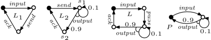
Figure 1: Four reactive and fully-probabilistic LPTSes.

Figure 1 illustrates LPTSes. Throughout this paper, we use filled circles to denote start states in the pictorial representations of LTPSes. For the distribution $\mu=\{(s_{1},0.1),(s_{2},0.9)\}$, $L_{2}$ in the figure has the transition $s_{1}\xrightarrow{output}\mu$. All the LPTSes in the figure are reactive as no state has more than one transition on a given action. They are also fully-probabilistic as no state has more than one transition. In the literature, an LPTS is also called a simple probabilistic automaton [20]. Similarly, a reactive (fully-probabilistic) LPTS is also called a (Labeled) Markov Decision Process (Markov Chain). Also, note that an LPTS with all the distributions restricted to Dirac distributions is the classical (non-probabilistic) Labeled Transition System (LTS); thus a reactive LTS corresponds to the standard notion of a deterministic LTS. For example, $L_{1}$ in Figure 1 is a reactive (or deterministic) LTS. We only consider finite state, finite alphabet and finitely branching (i.e. finitely many transitions from any state) LPTSes.

We are also interested in LPTSes with a tree structure, i.e. the start state is not in the support of any distribution and every other state is in the support of exactly one distribution. We call such LPTSes stochastic trees or simply, trees.

We use $\langle S_{i},s^{0}_{i},\alpha_{i},\tau_{i}\rangle$ for an LPTS $L_{i}$ and $\langle S_{L},s^{0}_{L},\alpha_{L},\tau_{L}\rangle$ for an LPTS $L$. The following notation is used in Section 5.

Notation 1

For an LPTS $L$ and an alphabet $\alpha$ with $\alpha_{L}\subseteq\alpha$, $L^{\alpha}$ stands for the LPTS $\langle S_{L},s^{0}_{L},\alpha,\tau_{L}\rangle$.

Let $L_{1}$ and $L_{2}$ be two LPTSes and $\mu_{1}\in\text{\em Dist}(S_{1})$, $\mu_{2}\in\text{\em Dist}(S_{2})$.

Definition 2 (Product [20])

The product of $\mu_{1}$ and $\mu_{2}$, denoted $\mu_{1}\otimes\mu_{2}$, is a distribution in $\text{\em Dist}(S_{1}\times S_{2})$, such that $\mu_{1}\otimes\mu_{2}:(s_{1},s_{2})\mapsto\mu_{1}(s_{1})\cdot\mu_{2}(s_{2})$.

Definition 3 (Composition [20])

The parallel composition of $L_{1}$ and $L_{2}$, denoted $L_{1}\parallel L_{2}$, is defined as the LPTS $\langle S_{1}\times S_{2},(s^{0}_{1},s^{0}_{2}),\alpha_{1}\cup\alpha_{2},\tau\rangle$ where $((s_{1},s_{2}),a,\mu)\in\tau$ iff

1. $s_{1}\xrightarrow{a}\mu_{1}$, $s_{2}\xrightarrow{a}\mu_{2}$ and $\mu=\mu_{1}\otimes\mu_{2}$, or

2. $s_{1}\xrightarrow{a}\mu_{1}$, $a\not\in\alpha_{2}$ and $\mu=\mu_{1}\otimes\delta_{s_{2}}$, or

3. $a\not\in\alpha_{1}$, $s_{2}\xrightarrow{a}\mu_{2}$ and $\mu=\delta_{s_{1}}\otimes\mu_{2}$.

For example, in Figure 1, $L$ is the composition of $L_{1}$ and $L_{2}$.

Strong Simulation. For two LTSes, a pair of states belonging to a strong simulation relation depends on whether certain other pairs of successor states also belong to the relation [17]. For LPTSes, one has successor distributions instead of successor states; a pair of states belonging to a strong simulation relation $R$ should now depend on whether certain other pairs in the supports of the successor distributions also belong to $R$. Therefore we define a binary relation on distributions, $\sqsubseteq_{R}$, which depends on the relation $R$ between states. Intuitively, two distributions can be related if we can pair the states in their support sets, the pairs contained in $R$, matching all the probabilities under the distributions.

Consider an example with $sRt$ and the transitions $s\xrightarrow{a}\mu_{1}$ and $t\xrightarrow{a}\mu_{2}$ with $\mu_{1}$ and $\mu_{2}$ as in Figure 2(a). In this case, one easy way to match the probabilities is to pair $s_{1}$ with $t_{1}$ and $s_{2}$ with $t_{2}$. This is sufficient if $s_{1}Rt_{1}$ and $s_{2}Rt_{2}$ also hold, in which case, we say that $\mu_{1}\sqsubseteq_{R}\mu_{2}$. However, such a direct matching may not be possible in general, as is the case in Figure 2(b). One can still obtain a matching by splitting the probabilities under the distributions in such a way that one can then directly match the probabilities as in Figure 2(a). Now, if $s_{1}Rt_{1}$, $s_{1}Rt_{2}$, $s_{2}Rt_{2}$ and $s_{2}Rt_{3}$ also hold, we say that $\mu_{1}\sqsubseteq_{R}\mu_{2}$. Note that there can be more than one possible splitting. This is the central idea behind the following definition where the splitting is achieved by a weight function. Let $R\subseteq S_{1}\times S_{2}$.

(a)

(b)

Figure 2: Explaining $\mu_{1}\sqsubseteq_{R}\mu_{2}$ by means of splitting (indicated by arrows) and matching (indicated by solid lines) the probabilities.

Definition 4 ([20])

$\mu_{1}\sqsubseteq_{R}\mu_{2}$ iff there is a weight function $w:S_{1}\times S_{2}\rightarrow\mathbb{Q}\cap[0,1]$ such that

1. $\mu_{1}(s_{1})=\sum_{s_{2}\in S_{2}}w(s_{1},s_{2})$ for all $s_{1}\in S_{1}$,

2. $\mu_{2}(s_{2})=\sum_{s_{1}\in S_{1}}w(s_{1},s_{2})$ for all $s_{2}\in S_{2}$,

3. $w(s_{1},s_{2})>0$ implies $s_{1}Rs_{2}$ for all $s_{1}\in S_{1}$, $s_{2}\in S_{2}$.

$\mu_{1}\sqsubseteq_{R}\mu_{2}$ can be checked by computing the maxflow in an appropriate network and checking if it equals $1.0$ [1]. If $\mu_{1}\sqsubseteq_{R}\mu_{2}$ holds, $w$ in the above definition is one such maxflow function. As explained above, $\mu_{1}\sqsubseteq_{R}\mu_{2}$ can be understood as matching all the probabilities (after splitting appropriately) under $\mu_{1}$ and $\mu_{2}$. Considering $\text{{\em Supp}}(\mu_{1})$ and $\text{{\em Supp}}(\mu_{2})$ as two partite sets, this is the weighted analog of saturating a partite set in bipartite matching, giving us the following analog of the well-known Hall’s Theorem for saturating $\text{{\em Supp}}(\mu_{1})$.

Lemma 1 ([21])

$\mu_{1}\sqsubseteq_{R}\mu_{2}$ iff for every $S\subseteq\text{{\em Supp}}(\mu_{1})$, $\mu_{1}(S)\leq\mu_{2}(R(S))$.

It follows that when $\mu_{1}\not\sqsubseteq_{R}\mu_{2}$, there exists a witness $S\subseteq\text{{\em Supp}}(\mu_{1})$ such that $\mu_{1}(S)>\mu_{2}(R(S))$. For example, if $R(s_{2})=\emptyset$ in Figure 2(a), its probability $\frac{1}{2}$ under $\mu_{1}$ cannot be matched and $S=\{s_{2}\}$ is a witness subset.

Definition 5 (Strong Simulation [20])

$R$ is a strong simulation iff for every $s_{1}Rs_{2}$ and $s_{1}\xrightarrow{a}\mu^{a}_{1}$ there is a $\mu^{a}_{2}$ with $s_{2}\xrightarrow{a}\mu^{a}_{2}$ and $\mu^{a}_{1}\sqsubseteq_{R}\mu^{a}_{2}$.

For $s_{1}\in S_{1}$ and $s_{2}\in S_{2}$, $s_{2}$ strongly simulates $s_{1}$, denoted $s_{1}\preceq s_{2}$, iff there is a strong simulation $T$ such that $s_{1}Ts_{2}$. $L_{2}$ strongly simulates $L_{1}$, also denoted $L_{1}\preceq L_{2}$, iff $s^{0}_{1}\preceq s^{0}_{2}$.

When checking a specification $P$ of a system $L$ with $\alpha_{P}\subset\alpha_{L}$, we implicitly assume that $P$ is completed by adding Dirac self-loops on each of the actions in $\alpha_{L}\setminus\alpha_{P}$ from every state before checking $L\preceq P$. For example, $L\preceq P$ in Figure 1 assuming that $P$ is completed with $\{\text{{\em send}},\text{{\em ack}}\}$. Checking $L_{1}\preceq L_{2}$ is decidable in polynomial time [1, 21] and can be performed with a greatest fixed point algorithm that computes the coarsest simulation between $L_{1}$ and $L_{2}$. The algorithm uses a relation variable $R$ initialized to $S_{1}\times S_{2}$ and checks the condition in Definition 5 for every pair in $R$, iteratively, removing any violating pairs from $R$. The algorithm terminates when a fixed point is reached showing $L_{1}\preceq L_{2}$ or when the pair of initial states is removed showing $L_{1}\not\preceq L_{2}$. If $n=\text{{\tt max}}(|S_{1}|,|S_{2}|)$ and $m=\text{{\tt max}}(|\tau_{1}|,|\tau_{2}|)$, the algorithm takes $O((mn^{6}+m^{2}n^{3})/\log n)$ time and $O(mn+n^{2})$ space [1]. Several optimizations exist [21] but we do not consider them here, for simplicity.

We do consider a specialized algorithm for the case that $L_{1}$ is a tree which we use during abstraction refinement (Sections 4 and 5). It initializes $R$ to $S_{1}\times S_{2}$ and is based on a bottom-up traversal of $L_{1}$. Let $s_{1}\in S_{1}$ be a non-leaf state during such a traversal and let $s_{1}\xrightarrow{a}\mu_{1}$. For every $s_{2}\in S_{2}$, the algorithm checks if there exists $s_{2}\xrightarrow{a}\mu_{2}$ with $\mu_{1}\sqsubseteq_{R}\mu_{2}$ and removes $(s_{1},s_{2})$ from $R$, otherwise, where $R$ is the current relation. This constitutes an iteration in the algorithm. The algorithm terminates when $(s^{0}_{1},s^{0}_{2})$ is removed from $R$ or when the traversal ends. Correctness is not hard to show and we skip the proof.

Lemma 2 ([20])

$\preceq$ is a preorder $($i.e. reflexive and transitive$)$ and is compositional, i.e. if $L_{1}\preceq L_{2}$ and $\alpha_{2}\subseteq\alpha_{1}$, then for every LPTS $L$, $L_{1}\parallel L\preceq L_{2}\parallel L$.

Finally, we show the soundness and completeness of the rule ASym. The rule is sound if the conclusion holds whenever there is an $A$ satisfying the premises. And the rule is complete if there is an $A$ satisfying the premises whenever the conclusion holds.

Theorem 2.1

For $\alpha_{A}\subseteq\alpha_{2}$, the rule ASym is sound and complete.

Proof

Soundness follows from Lemma 2. Completeness follows trivially by replacing $A$ with $L_{2}$. ∎

3 Counterexamples to Strong Simulation

Let $L_{1}$ and $L_{2}$ be two LPTSes. We characterize a counterexample to $L_{1}\preceq L_{2}$ as a tree and show that any simpler structure is not sufficient in general. We first describe counterexamples via a simple language-theoretic characterization.

Definition 6 (Language of an LPTS)

Given an LPTS $L$, we define its language, denoted $\mathcal{L}(L)$, as the set $\{L^{\prime}|L^{\prime}~{}\text{is an LPTS and }L^{\prime}\preceq L\}$.

Lemma 3

$L_{1}\preceq L_{2}$ iff $\mathcal{L}(L_{1})\subseteq\mathcal{L}(L_{2})$.

Proof

Necessity follows trivially from the transitivity of $\preceq$ and sufficiency follows from the reflexivity of $\preceq$ which implies $L_{1}\in\mathcal{L}(L_{1})$. ∎

Thus, a counterexample $C$ can be defined as follows.

Definition 7 (Counterexample)

A counterexample to $L_{1}\preceq L_{2}$ is an LPTS $C$ such that $C\in\mathcal{L}(L_{1})\setminus\mathcal{L}(L_{2})$, i.e. $C\preceq L_{1}$ but $C\not\preceq L_{2}$.

Now, $L_{1}$ itself is a trivial choice for $C$ but it does not give any more useful information than what we had before checking the simulation. Moreover, it is preferable to have $C$ with a special and simpler structure rather than a general LPTS as it helps in a more efficient counterexample analysis, wherever it is used. When the LPTSes are restricted to LTSes, a tree-shaped LTS is known to be sufficient as a counterexample [5]. Based on a similar intuition, we show that a stochastic tree is sufficient as a counterexample in the probabilistic case.

Theorem 3.1

If $L_{1}\not\preceq L_{2}$, there is a tree which serves as a counterexample.

Proof

We only give a brief sketch of a constructive proof here. See Appendix for a detailed proof. Counterexample generation is based on the coarsest strong simulation computation from Section 2. By induction on the number of pairs not in the current relation $R$, we show that there is a tree counterexample to $s_{1}\preceq s_{2}$ whenever $(s_{1},s_{2})$ is removed from $R$. We only consider the inductive case here. The pair is removed because there is a transition $s_{1}\xrightarrow{a}\mu_{1}$ but for every $s_{2}\xrightarrow{a}\mu$, $\mu_{1}\not\sqsubseteq_{R}\mu$ i.e. there exists $S^{\mu}_{1}\subseteq\text{{\em Supp}}(\mu_{1})$ such that $\mu_{1}(S^{\mu}_{1})>\mu(R(S^{\mu}_{1}))$. Such an $S^{\mu}_{1}$ can be found using Algorithm 1. Now, no pair in $S^{\mu}_{1}\times(\text{{\em Supp}}(\mu)\setminus R(S^{\mu}_{1}))$ is in $R$. By induction hypothesis, a counterexample tree exists for each such pair. A counterexample to $s_{1}\preceq s_{2}$ is built using $\mu_{1}$ and all these other trees. ∎

Algorithm 1 Finding $T\subseteq S_{1}$ such that $\mu_{1}(T)>\mu(R(T))$.

Given $\mu_{1}\in\text{\em Dist}(S_{1})$, $\mu\in\text{\em Dist}(S_{2})$, $R\subseteq S_{1}\times S_{2}$ with $\mu_{1}\not\sqsubseteq_{R}\mu$.

1:  let $f$ be a maxflow function for the flow network corresponding to $\mu_{1}$ and $\mu$

2:  find $s_{1}\in S_{1}$ with $\mu_{1}(s_{1})>\sum_{s_{2}\in S_{2}}f(s_{1},s_{2})$ and let $T=\{s_{1}\}$

3:  while $\mu_{1}(T)\leq\mu(R(T))$ do

4:     $T\leftarrow\{s_{1}\in S_{1}|\exists s_{2}\in R(T):f(s_{1},s_{2})>0\}$

5:  end while

6:  return  $T$

For an illustration, see Figure 3 where $C$ is a counterexample to $L_{1}\preceq L_{2}$. Algorithm 1 is also analogous to the one used to find a subset failing Hall’s condition in Graph Theory and can easily be proved correct. We obtain the following complexity bounds whose proof can be found in Appendix.

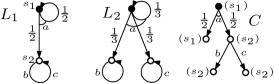
Figure 3: $C$ is a counterexample to $L_{1}\preceq L_{2}$.

Theorem 3.2

Deciding $L_{1}\preceq L_{2}$ and obtaining a tree counterexample takes $O(mn^{6}+m^{2}n^{3})$ time and $O(mn+n^{2})$ space where $n=\text{{\tt max}}(|S_{L_{1}}|,|S_{L_{2}}|)$ and $m=\text{{\tt max}}(|\tau_{1}|,|\tau_{2}|)$.

Note that the obtained counterexample is essentially a finite tree execution of $L_{1}$. That is, there is a total mapping $M:S_{C}\to S_{1}$ such that for every transition $c\xrightarrow{a}\mu_{c}$ of $C$, there exists $M(c)\xrightarrow{a}\mu_{1}$ such that $M$ restricted to $\text{{\em Supp}}(\mu_{c})$ is an injection and for every $c^{\prime}\in\text{{\em Supp}}(\mu_{c})$, $\mu_{c}(c^{\prime})=\mu_{1}(M(c^{\prime}))$. $M$ is also a strong simulation. We call such a mapping an execution mapping from $C$ to $L_{1}$. Figure 3 shows an execution mapping in brackets beside the states of $C$. We therefore have the following corollary.

Corollary 1

If $L_{1}$ is reactive and $L_{1}\not\preceq L_{2}$, there is a reactive tree which serves as a counterexample.

The following two lemmas show that (reactive) trees are the simplest structured counterexamples (proofs in Appendix).

Lemma 4

There exist reactive LPTSes $R_{1}$ and $R_{2}$ such that $R_{1}\not\preceq R_{2}$ and no counterexample is fully-probabilistic.

Thus, if $L_{1}$ is reactive, a reactive tree is the simplest structure for a counterexample to $L_{1}\preceq L_{2}$. This is surprising, since the non-probabilistic counterpart of a fully-probabilistic LPTS is a trace of actions and it is known that trace inclusion coincides with simulation conformance between reactive (i.e. deterministic) LTSes. If there is no such restriction on $L_{1}$, one may ask if a reactive LPTS suffices as a counterexample to $L_{1}\preceq L_{2}$. That is not the case either, as the following lemma shows.

Lemma 5

There exist an LPTS $L$ and a reactive LPTS $R$ such that $L\not\preceq R$ and no counterexample is reactive.

4 CEGAR for Checking Strong Simulation

Now that the notion of a counterexample has been formalized, we describe a CounterExample Guided Abstraction Refinement (CEGAR) approach [6] to check $L\preceq P$ where $L$ and $P$ are LPTSes and $P$ stands for a specification of $L$. We will use this approach to describe AGAR in the next section.

Abstractions for $L$ are obtained using a quotient construction from a partition $\Pi$ of $S_{L}$. We let $\Pi$ also denote the corresponding set of equivalence classes and given an arbitrary $s\in S$, let $[s]_{\Pi}$ denote the equivalence class containing $s$. The quotient is an adaptation of the usual construction in the non-probabilistic case.

Definition 8 (Quotient LPTS)

Given a partition $\Pi$ of $S_{L}$, define the quotient LPTS, denoted $L/\Pi$, as the LPTS $\langle\Pi,[s^{0}_{L}]_{\Pi},\alpha_{L},\tau\rangle$ where $(c,a,\mu_{l})\in\tau$ iff $(s,a,\mu)\in\tau_{L}$ for some $s\in S_{L}$ with $s\in c$ and $\mu_{l}(c^{\prime})=\sum_{t\in c^{\prime}}\mu(t)$ for all $c^{\prime}\in\Pi$.

As the abstractions are built from an explicit representation of $L$, this is not immediately useful. But, as we will see in Sections 5 and 6, this becomes very useful when adapted to the assume-guarantee setting.

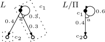
Figure 4: An LPTS $L$, partition $\Pi=\{c_{1},c_{2}\}$ and the quotient $L/\Pi$.

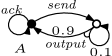
Figure 5: An assumption for $L_{1}$, $L_{2}$ and $P$
in Figure 1.

Figure 5 shows an example quotient. Note that $L\preceq L/\Pi$ for any partition $\Pi$ of $S_{L}$ (proof in Appendix), with the relation $R=\{(s,c)|s\in c,c\in\Pi\}$ as a strong simulation.

Algorithm 2 CEGAR for LPTSes: checks $L\preceq P$

1:  $A\leftarrow L/\Pi$, where $\Pi$ is the coarsest partition of $S_{L}$

2:  while $A\not\preceq P$ do

3:     obtain a counterexample $C$

4:     $(spurious,A^{\prime})\leftarrow\text{{\em analyzeAndRefine}}(C,A,L)$ {see text}

5:     if $spurious$ then

6:        $A\leftarrow A^{\prime}$

7:     else

8:        return  counterexample $C$

9:     end if

10:  end while

11:  return  $L\preceq P$ holds

CEGAR for LPTSes is sketched in Algorithm 2. It maintains an abstraction $A$ of $L$, initialized to the quotient for the coarsest partition, and iteratively refines $A$ based on the counterexamples obtained from the simulation check against $P$ until a partition whose corresponding quotient conforms to $P$ w.r.t. $\preceq$ is obtained, or a real counterexample is found. In the following, we describe how to analyze if a counterexample is spurious, due to abstraction, and how to refine the abstraction in case it is (lines $4-6$). Our analysis is an adaptation of an existing one for counterexamples which are arbitrary sub-structures of $A$ [3]; while our tree counterexamples have an execution mapping to $A$, they are not necessarily sub-structures of $A$.

Analysis and Refinement (analyzeAndRefine$(\cdot)$). Assume that $\Pi$ is a partition of $S_{L}$ such that $A=L/\Pi$ and $A\not\preceq P$. Let $C$ be a tree counterexample obtained by the algorithm described in Section 3, i.e. $C\preceq A$ but $C\not\preceq P$. As described in Section 3, there is an execution mapping $M:S_{C}\to S_{A}$ which is also a strong simulation. Let $R_{M}\subseteq S_{C}\times S_{L}$ be $\{(s_{1},s_{2})|s_{1}M[s_{2}]_{\Pi}\}$. Our refinement strategy tries to obtain the coarsest strong simulation between $C$ and $L$ contained in $R_{M}$, using the specialized algorithm for trees described in Section 2 with $R_{M}$ as the initial candidate. Let $R$ and $R_{\text{{\em old}}}$ be the candidate relations at the end of the current and the previous iterations, respectively, and let $s_{1}\xrightarrow{a}\mu_{1}$ be the transition in $C$ considered by the algorithm in the current iteration. ($R_{\text{{\em old}}}$ is undefined initially.) The strategy refines a state when one of the following two cases happens before termination and otherwise, returns $C$ as a real counterexample.

1. $R(s_{1})=\emptyset$. There are two possible reasons for this case. One is that the states in $\text{{\em Supp}}(\mu_{1})$ are not related, by $R$, to enough number of states in $S_{L}$ (i.e. $\mu_{1}$ is spurious) and (the images under $M$ of) all the states in $\text{{\em Supp}}(\mu_{1})$ are candidates for refinement. The other possible reason is the branching (more than one transition) from $s_{1}$ where no state in $R_{M}(s_{1})$ can simulate all the transitions of $s_{1}$ and $M(s_{1})$ is a candidate for refinement.

2. $M(s_{1})=[s^{0}_{L}]_{\Pi}$, $s^{0}_{L}\in R_{\text{{\em old}}}(s_{1})\setminus R(s_{1})$ and $R(s_{1})\neq\emptyset$, i.e. $M(s_{1})$ is the initial state of $A$ but $s_{1}$ is no longer related to $s^{0}_{L}$ by $R$. Here, $M(s_{1})$ is a candidate for refinement.

In case $1$, our refinement strategy first tries to split the equivalence class $M(s_{1})$ into $R_{\text{{\em old}}}(s_{1})$ and the rest and then, for every state $s\in\text{{\em Supp}}(\mu_{1})$, tries to split the equivalence class $M(s)$ into $R_{\text{{\em old}}}(s)$ and the rest, unless $M(s)=M(s_{1})$ and $M(s_{1})$ has already been split. And in case $2$, the strategy splits the equivalence class $M(s_{1})$ into $R_{\text{{\em old}}}(s_{1})\setminus R(s_{1})$ and the rest. It follows from the two cases that if $C$ is declared real, then $C\preceq L$ with the final $R$ as a strong simulation between $C$ and $L$ and hence, $C$ is a counterexample to $L\preceq P$. The following lemma (proof in Appendix) shows that the refinement strategy always leads to progress.

Lemma 6

The above refinement strategy always results in a strictly finer partition $\Pi^{\prime}<\Pi$.

5 Assume-Guarantee Abstraction Refinement

We now describe our approach to Assume-Guarantee Abstraction Refinement (AGAR) for LPTSes. The approach is similar to CEGAR from the previous section with the notable exception that counterexample analysis is performed in an assume guarantee style: a counterexample obtained from checking one component is used to refine the abstraction of a different component.

Given LPTSes $L_{1}$, $L_{2}$ and $P$, the goal is to check $L_{1}\parallel L_{2}\preceq P$ in an assume-guarantee style, using rule ASym. The basic idea is to maintain $A$ in the rule as an abstraction of $L_{2}$, i.e. the second premise holds for free throughout, and to check only the first premise for every $A$ generated by the algorithm. As in CEGAR, we restrict $A$ to the quotient for a partition of $S_{2}$. If the first premise holds for an $A$, then $L_{1}\parallel L_{2}\preceq P$ also holds, by the soundness of the rule. Otherwise, the obtained counterexample $C$ is analyzed to see whether it indicates a real error or it is spurious, in which case $A$ is refined (as described in detail below). Algorithm 3 sketches the AGAR loop.

For an example, $A$ in Figure 5 shows the final assumption generated by AGAR for the LPTSes in Figure 1 (after one refinement).

Algorithm 3 AGAR for LPTSes: checks $L_{1}\parallel L_{2}\preceq P$

1:  $A\leftarrow$ coarsest abstraction of $L_{2}$

2:  while $L_{1}\parallel A\not\preceq P$ do

3:     obtain a counterexample $C$

4:     obtain projections $C\upharpoonright_{L_{1}}$ and $C\upharpoonright_{A}$

5:     $(\text{\em spurious},A^{\prime})\leftarrow\text{{\em analyzeAndRefine}}(C\upharpoonright_{A},A,L_{2})$

6:     if spurious then

7:        $A\leftarrow A^{\prime}$

8:     else

9:        return  counterexample $C$

10:     end if

11:  end while

12:  return  $L_{1}\parallel L_{2}\preceq P$ holds

Analysis and Refinement. The counterexample analysis is performed compositionally, using the projections of $C$ onto $L_{1}$ and $A$. As there is an execution mapping from $C$ to $L_{1}\parallel A$, these projections are the contributions of $L_{1}$ and $A$ towards $C$ in the composition. We denote these projections by $C\upharpoonright_{L_{1}}$ and $C\upharpoonright_{A}$, respectively. In the non-probabilistic case, these are obtained by simply projecting $C$ onto the respective alphabets. In the probabilistic scenario, however, composition changes the probabilities in the distributions (Definition 2) and alphabet projection is insufficient. For this reason, we additionally record the individual distributions of the LPTSes responsible for a product distribution while performing the composition. Thus, projections $C\upharpoonright_{L_{1}}$ and $C\upharpoonright_{A}$ can be obtained using this auxiliary information. Note that there is a natural execution mapping from $C\upharpoonright_{A}$ to $A$ and from $C\upharpoonright_{L_{1}}$ to $L_{1}$. We can then employ the analysis described in Section 4 between $C\upharpoonright_{A}$ and $A$, i.e. invoke $\text{{\em analyzeAndRefine}}(C\upharpoonright_{A},A,L_{2})$ to determine if $C\upharpoonright_{A}$ (and hence, $C$) is spurious and to refine $A$ in case it is. Otherwise, $C\upharpoonright_{A}\preceq L_{2}$ and hence, $(C\upharpoonright_{A})^{\alpha_{2}}\preceq L_{2}$. Together with $(C\upharpoonright_{L_{1}})^{\alpha_{1}}\preceq L_{1}$ this implies $(C\upharpoonright_{L_{1}})^{\alpha_{1}}\parallel(C\upharpoonright_{A})^{\alpha_{2}}\preceq L_{1}\parallel L_{2}$ (Lemma 2). As $C\preceq(C\upharpoonright_{L_{1}})^{\alpha_{1}}\parallel(C\upharpoonright_{A})^{\alpha_{2}}$, $C$ is then a real counterexample. Thus, we have the following result.

Theorem 5.1 (Correctness and Termination)

Algorithm AGAR always terminates with at most $|S_{2}|-1$ refinements and $L_{1}\parallel L_{2}\not\preceq P$ if and only if the algorithm returns a real counterexample.

Proof

Correctness: AGAR terminates when either Premise 1 is satisfied by the current assumption (line $12$) or when a counterexample is returned (line $9$). In the first case, we know that Premise 2 holds by construction and since ASym is sound (Theorem 2.1) it follows that indeed $L_{1}\|L_{2}\preceq P$. In the second case, the counterexample returned by AGAR is real (see above) showing that $L_{1}\parallel L_{2}\not\preceq P$.

Termination: AGAR iteratively refines the abstraction until the property holds or a real counterexample is reported. Abstraction refinement results in a finer partition (Lemma 6) and thus it is guaranteed to terminate since in the worst case $A$ converges to $L_{2}$ which is finite state. Since rule ASym is trivially complete for $L_{2}$ (proof of Theorem 2.1) it follows that AGAR will also terminate, and the number of refinements is bounded by $|S_{2}|-1$. ∎

In practice, we expect AGAR to terminate earlier than in $|S_{2}|-1$ steps, with an assumption smaller than $L_{2}$. AGAR will terminate as soon as it finds an assumption that satisfies the premises or that helps exhibit a real counterexample. Note also that, although AGAR uses an explicit representation for the individual components, it never builds $L_{1}\parallel L_{2}$ directly (except in the worst-case) keeping the cost of verification low.

Reasoning with $n\geq 2$ Components. So far, we have discussed compositional verification in the context of two components $L_{1}$ and $L_{2}$. This reasoning can be generalized to $n\geq 2$ components using the following (sound and complete) rule.

$$\displaystyle{\hbox{\hskip 121.19737pt\vbox{\hbox{\hskip-121.19736pt\hbox{\hbox{$\displaystyle\displaystyle 1:L_{1}\parallel A_{1}\preceq P$}\hskip 20.00003pt\hbox{\hbox{$\displaystyle\displaystyle 2:L_{2}\parallel A_{2}\preceq A_{1}$}\hskip 20.00003pt\hbox{\hbox{$\displaystyle\displaystyle...$}\hskip 20.00003pt\hbox{\hbox{$\displaystyle\displaystyle n:L_{n}\preceq A_{n-1}$}}}}}}\vbox{}}}\over\hbox{\hskip 21.70322pt\vbox{\vbox{}\hbox{\hskip-21.7032pt\hbox{\hbox{$\displaystyle\displaystyle\parallel_{i=1}^{n}L_{i}\preceq P$}}}}}} ( )$$ ASym-N

The rule enables us to overcome the intermediate state explosion that may be associated with two-way decompositions (when the subsystems are larger than the entire system). The AGAR algorithm for this rule involves the creation of $n-1$ nested instances of AGAR for two components, with the $i$th instance computing the assumption $A_{i}$ for $(L_{1}\parallel\dots\parallel L_{i})\parallel(L_{i+1}\parallel A_{i+1})\preceq P$. When the AGAR instance for $A_{i-1}$ returns a counterexample $C$, for $1<i\leq n-1$, we need to analyze $C$ for spuriousness and refine $A_{i}$ in case it is. From Algorithm 3, $C$ is returned only if analyzeAndRefine$(C\upharpoonright_{A_{i-1}},A_{i-1},L_{i}\parallel A_{i})$ concludes that $C\upharpoonright_{A_{i-1}}$ is real (note that $A_{i-1}$ is an abstraction of $L_{i}\parallel A_{i}$). From analyzeAndRefine in Section 4, this implies that the final relation $R$ computed between the states of $C\upharpoonright_{A_{i-1}}$ and $L_{i}\parallel A_{i}$ is a strong simulation between them. It follows that, although $C\upharpoonright_{A_{i-1}}$ does not have an execution mapping to $L_{i}\parallel A_{i}$, we can naturally obtain a tree $T$ using $C\upharpoonright_{A_{i-1}}$, via $R$, with such a mapping. Thus, we modify the algorithm to return $T\upharpoonright_{A_{i}}$ at line $9$, instead of $C$, which can then be used to check for spuriousness and refine $A_{i}$. Note that when $A_{i}$ is refined, all the $A_{j}$’s for $j<i$ need to be recomputed.

Compositional Verification of Logical Properties. AGAR can be further applied to automate assume-guarantee checking of properties $\phi$ written as formulae in a logic that is preserved by strong simulation such as the weak-safety fragment of probabilistic CTL (pCTL) [3] which also yield trees as counterexamples. The rule ASym is both sound and complete for this logic ($\models$ denotes property satisfaction) for $\alpha_{A}\subseteq\alpha_{2}$ with a proof similar to that of Theorem 2.1.

$$\displaystyle{\hbox{\hskip 58.83456pt\vbox{\hbox{\hskip-58.83455pt\hbox{\hbox{$\displaystyle\displaystyle 1:L_{1}\parallel A\models\phi$}\hskip 20.00003pt\hbox{\hbox{$\displaystyle\displaystyle 2:L_{2}\preceq A$}}}}\vbox{}}}\over\hbox{\hskip 21.3347pt\vbox{\vbox{}\hbox{\hskip-21.33469pt\hbox{\hbox{$\displaystyle\displaystyle L_{1}\parallel L_{2}\models\phi$}}}}}}$$

$A$ can be computed as a conservative abstraction of $L_{2}$ and iteratively refined based on the tree counterexamples to premise $1$, using the same procedures as before. The rule can be generalized to reasoning about $n\geq 2$ components as described above and also to richer logics with more general counterexamples adapting existing CEGAR approaches [3] to AGAR. We plan to further investigate this direction in the future.

6 Implementation and Results

Implementation. We implemented the algorithms for checking simulation (Section 2), for generating counterexamples (as in the proof of Lemma 3.1) and for AGAR (Algorithm 3) with ASym and ASym-N in Java${}^{\text{TM}}$ . We used the front-end of PRISM’s [15] explicit-state engine to parse the models of the components described in PRISM’s input language and construct LPTSes which were then handled by our implementation.

While the Java${}^{\text{TM}}$ implementation for checking simulation uses the greatest fixed point computation to obtain the coarsest strong simulation, we noticed that the problem of checking the existence of a strong simulation is essentially a constraint satisfaction problem. To leverage the efficient constraint solvers that exist today, we reduced the problem of checking simulation to an SMT problem with rational linear arithmetic as follows. For every pair of states, the constraint that the pair is in some strong simulation is simply the encoding of the condition in Definition 5. For a relevant pair of distributions $\mu_{1}$ and $\mu_{2}$, the constraint for $\mu_{1}\sqsubseteq_{R}\mu_{2}$ is encoded by means of a weight function (as given by Definition 4) and the constraint for $\mu_{1}\not\sqsubseteq_{R}\mu_{2}$ is encoded by means of a witness subset of $\text{{\em Supp}}(\mu_{1})$ (as in Lemma 1), where $R$ is the variable for the strong simulation. We use Yices (v$1.0.29$) [9] to solve the resulting SMT problem; a real variable in Yices input language is essentially a rational variable. There is no direct way to obtain a tree counterexample when the SMT problem is unsatisfiable. Therefore when the conformance fails, we obtain the unsat core from Yices, construct the sub-structure of $L_{1}$ (when we check $L_{1}\preceq L_{2}$) from the constraints in the unsat core and check the conformance of this sub-structure against $L_{2}$ using the Java${}^{\text{TM}}$ implementation. This sub-structure is usually much smaller than $L_{1}$ and contains only the information necessary to expose the counterexample.

Results. We evaluated our algorithms using this implementation on several examples analyzed in previous work [11]. Some of these examples were created by introducing probabilistic failures into non-probabilistic models used earlier [19] while others were adapted from PRISM benchmarks [15]. The properties used previously were about probabilistic reachability and we had to create our own specification LPTSes after developing an understanding of the models. The models in all the examples satisfy the respective specifications. We briefly describe the models and the specifications below, all of which are available at http://www.cs.cmu.edu/~akomurav/publications/agar/AGAR.html.

CS₁ and CS_N model a Client-Server protocol with mutual exclusion having probabilistic failures in one or all of the $N$ clients, respectively. The specifications describe the probabilistic failure behavior of the clients while hiding some of the actions as is typical in a high level design specification.

MER models a resource arbiter module of NASA’s software for Mars Exploration Rovers which grants and rescinds shared resources for several users. We considered the case of two resources with varying number of users and probabilistic failures introduced in all the components. As in the above example, the specifications describe the probabilistic failure behavior of the users while hiding some of the actions.

SN models a wireless Sensor Network of one or more sensors sending data and messages to a process via a channel with a bounded buffer having probabilistic behavior in the components. Creating specification LPTSes for this example turned out to be more difficult than the above examples, and we obtained them by observing the system’s runs and by manual abstraction.

Example			ASym						ASym-N					Mono
$($param$)$	$|L|$	$|P|$	$|L_{1}|$	$|L_{2}|$	Time	Mem	$|L_{M}|$	$|A_{M}|$	$|L_{c}|$	Time	Mem	$|L_{M}|$	$|A_{M}|$	Time	Mem
CS${}_{1}(5)$	${\bf 94}$	$16$	$36$	$405$	$7.2$	$15.6$	$182$	$33$	$36$	$74.0$	$15.1$	$182$	$34$	${\bf 0.2}$	${\bf 8.8}$
CS${}_{1}(6)$	${\bf 136}$	$19$	$49$	$1215$	$11.6$	$22.7$	$324$	$41$	$49$	$810.7$	$21.4$	$324$	$40$	${\bf 0.5}$	${\bf 12.2}$
CS${}_{1}(7)$	${\bf 186}$	$22$	$64$	$3645$	$37.7$	$49.4$	$538$	$56$	$64$	out	–	–	–	${\bf 0.8}$	${\bf 17.9}$
CS${}_{N}(2)$	${\bf 34}$	$15$	$25$	$9$	$0.7$	$7.1$	$51$	$7$	$9$	$2.4$	$6.8$	$40$	$25$	${\bf 0.1}$	${\bf 5.9}$
CS${}_{N}(3)$	${\bf 184}$	$54$	$125$	$16$	$43.0$	$63.0$	$324$	$12$	$16$	$1.6k$	$109.6$	$372$	$125$	${\bf 14.8}$	${\bf 37.9}$
CS${}_{N}(4)$	${\bf 960}$	$189$	$625$	$25$	out	–	–	–	$25$	out	–	–	–	${\bf 1.8}k$	${\bf 667.5}$
MER $(3)$	$16k$	$12$	$278$	$1728$	${\bf 2.6}$	$19.7$	${\bf 706}$	$7$	$278$	$3.6$	${\bf 14.6}$	${\bf 706}$	$7$	$193.8$	$458.5$
MER $(4)$	$120k$	$15$	$465$	$21k$	${\bf 15.0}$	$53.9$	${\bf 2}k$	$11$	$465$	$34.7$	${\bf 37.8}$	${\bf 2}k$	$11$	out	–
MER $(5)$	$841k$	$18$	$700$	$250k$	–	out	–	–	$700$	${\bf 257.8}$	${\bf 65.5}$	${\bf 3.3}k$	$16$	–	out
SN $(1)$	$462$	$18$	$43$	$32$	${\bf 0.2}$	${\bf 6.2}$	${\bf 43}$	$3$	$126$	$1.7$	$8.5$	$165$	$6$	$1.5$	$27.7$
SN $(2)$	$7860$	$54$	$796$	$32$	${\bf 79.5}$	${\bf 112.9}$	${\bf 796}$	$3$	$252$	$694.4$	$171.7$	$1.4k$	$21$	$4.7k$	$1.3k$
SN $(3)$	$78k$	$162$	$7545$	$32$	out	–	–	–	$378$	${\bf 7.2}k$	${\bf 528.8}$	${\bf 1.4}k$	$21$	–	out

Table 1: AGAR vs monolithic verification. ¹ Mem-out during model construction.

Table 1 shows the results we obtained when ASym and ASym-N were compared with monolithic (non-compositional) conformance checking. $|X|$ stands for the number of states of an LPTS $X$. $L$ stands for the whole system, $P$ for the specification, $L_{M}$ for the LPTS with the largest number of states built by composing LPTSes during the course of AGAR, $A_{M}$ for the assumption with the largest number of states during the execution and $L_{c}$ for the component with the largest number of states in ASym-N. Time is in seconds and Memory is in megabytes. We also compared $|L_{M}|$ with $|L|$, as $|L_{M}|$ denotes the largest LPTS ever built by AGAR. Best figures, among ASym, ASym-N and Mono, for Time, Memory and LPTS sizes, are boldfaced. All the results were taken on a Fedora-10 64-bit machine running on an Intel® Core${}^{\text{TM}}$2 Quad CPU of $2.83$GHz and $4$GB RAM. We imposed a $2$GB upper bound on Java heap memory and a $2$ hour upper bound on the running time. We observed that most of the time during AGAR was spent in checking the premises and an insignificant amount was spent for the composition and the refinement steps. Also, most of the memory was consumed by Yices. We tried several orderings of the components (the $L_{i}$’s in the rules) and report only the ones giving the best results.

While monolithic checking outperformed AGAR for Client-Server, there are significant time and memory savings for MER and Sensor Network where in some cases the monolithic approach ran out of resources (time or memory). One possible reason for AGAR performing worse for Client-Server is that $|L|$ is much smaller than $|L_{1}|$ or $|L_{2}|$. When compared to using ASym, ASym-N brings further memory savings in the case of MER and also time savings for Sensor Network with parameter $3$ which could not finish in $2$ hours when used with ASym. As already mentioned, these models were analyzed previously with an assume-guarantee framework using learning from traces [11]. Although that approach uses a similar assume-guarantee rule (but instantiated to check probabilistic reachability) and the results have some similarity (e.g. Client-Server is similarly not handled well by the compositional approach), we can not directly compare it with AGAR as it considers a different class of properties.

7 Conclusion and Future Work

We described a complete, fully automated abstraction-refinement approach for assume-guarantee checking of strong simulation between LPTSes. The approach uses refinement based on counterexamples formalized as stochastic trees and it further applies to checking safe-pCTL properties. We showed experimentally the merits of the proposed technique. We plan to extend our approach to cases where the assumption $A$ has a smaller alphabet than that of the component it represents as this can potentially lead to further savings. Strong simulation would no longer work and one would need to use weak simulation [20], for which checking algorithms are unknown yet. We would also like to explore symbolic implementations of our algorithms, for increased scalability. As an alternative approach, we plan to build upon our recent work [14] on learning LPTSes to develop practical compositional algorithms and compare with AGAR.

Acknowledgments.

We thank Christel Baier, Rohit Chadha, Lu Feng, Holger Hermanns, Marta Kwiatkowska, Joel Ouaknine, David Parker, Frits Vaandrager, Mahesh Viswanathan, James Worrell and Lijun Zhang for generously answering our questions related to this research. We also thank the anonymous reviewers for their suggestions and David Henriques for carefully reading an earlier draft.

Appendix 0.A Proof of Lemma 2

We first show that $\preceq$ is a preorder. Reflexivity can be easily proved by showing that the identity relation is a strong simulation. We only consider transitivity. Let $L_{1}\preceq L_{2}$ and $L_{2}\preceq L_{3}$. Thus, there are strong simulations $R_{12}\subseteq S_{1}\times S_{2}$ and $R_{23}\subseteq S_{2}\times S_{3}$. Consider the relation $R=\{(s_{1},s_{3})|\exists s_{2}:s_{1}R_{12}s_{2}~{}\text{and}~{}s_{2}R_{23}s_{3}\}$. Let $s_{1}Rs_{3}$ and $s_{1}\xrightarrow{a}\mu_{1}$. Also, let $s_{2}\in S_{2}$ be such that $s_{1}R_{12}s_{2}$ and $s_{2}R_{23}s_{3}$. As $R_{12}$ is a strong simulation, there exists $s_{2}\xrightarrow{a}\mu_{2}$ with $\mu_{1}\sqsubseteq_{R_{12}}\mu_{2}$. Again, as $R_{23}$ is a strong simulation, there exists $s_{3}\xrightarrow{a}\mu_{3}$ with $\mu_{2}\sqsubseteq_{R_{23}}\mu_{3}$. Now, let $S\subseteq\text{{\em Supp}}(\mu_{1})$ be arbitrary. We have $\mu_{1}(S)\leq\mu_{2}(R_{12}(S))\leq\mu_{3}(R_{23}(R_{12}(S)))=\mu_{3}(R(S))$ (Lemma 1). Thus, $\mu_{1}\sqsubseteq_{R}\mu_{3}$ and hence, $R$ is a strong simulation. Also, $s^{0}_{1}Rs^{0}_{3}$ by definition of $R$. We conclude that $L_{1}\preceq L_{3}$.

Now, we show that $\preceq$ is compositional. Assume $L_{1}\preceq L_{2}$ with $\alpha_{2}\subseteq\alpha_{1}$. Let $R_{12}\subseteq S_{1}\times S_{2}$ be a strong simulation. Consider the relation $R$ defined below.

$$R=\{((s_{1},s),(s_{2},s))|s_{1}R_{12}s_{2}~{}\text{and}~{}s\in S_{L}\}$$

Let $(s_{1},s)R(s_{2},s)$ and $(s_{1},s)\xrightarrow{a}\mu_{a}$. So, $s_{1}R_{12}s_{2}$. By Definition 3, there are three cases to analyze.

$s_{1}\xrightarrow{a}\mu_{1}$, $s\xrightarrow{a}\mu$ and $\mu_{a}=\mu_{1}\otimes\mu$ : As $R_{12}$ is a strong simulation, there exists $s_{2}\xrightarrow{a}\mu_{2}$ with $\mu_{1}\sqsubseteq_{R_{12}}\mu_{2}$. And by Definition 3, $(s_{2},s)\xrightarrow{a}\mu^{\prime}_{a}$ where $\mu^{\prime}_{a}=\mu_{2}\otimes\mu$. Now, let $X\subseteq\text{{\em Supp}}(\mu_{a})$. For each $s\in S_{L}$, let $X_{s}\subseteq X$ contain all the pairs of $X$ with $s$ as the second member. Thus, the $X_{s}$’s partition $X$. We have $\mu_{a}(X)$

$$=\sum_{s\in S_{L}}\mu_{a}(X_{s}\times\{s\})$$

$$=\sum_{s\in S_{L}}\mu_{1}(X_{s})\cdot\mu(s) \mu_{a}$$ definition of

$$\leq\sum_{s\in S_{L}}\mu_{2}(R_{12}(X_{s}))\cdot\mu(s) R_{12}$$ is a strong simulation

$$=\sum_{s\in S_{L}}\mu^{\prime}_{a}(R_{12}(X_{s})\times\{s\}) \mu^{\prime}_{a}$$ definition of

$$=\sum_{s\in S_{L}}\mu^{\prime}_{a}(R(X_{s}\times\{s\})) R$$ definition of

$$=\mu^{\prime}_{a}(\bigcup_{s\in S_{L}}R(X_{s}\times\{s\})) R(X_{s}\times\{s\}) s$$ the sets are disjoint for distinct

$$=\mu^{\prime}_{a}(R(\bigcup_{s\in S_{L}}X_{s}\times\{s\}))$$

$$=\mu^{\prime}_{a}(R(X))$$

which implies that $\mu_{a}\sqsubseteq_{R}\mu^{\prime}_{a}$.

$a\not\in\alpha_{1}$, $s\xrightarrow{a}\mu$ and $\mu_{a}=\delta_{s_{1}}\otimes\mu$ : As $\alpha_{2}\subseteq\alpha_{1}$, $a\not\in\alpha_{2}$ and by Definition 3, $(s_{2},s)\xrightarrow{a}\mu^{\prime}_{a}$ with $\mu^{\prime}_{a}=\delta_{s_{2}}\otimes\mu$. Now, let $X\subseteq\text{{\em Supp}}(\mu_{a})$ and let $X_{2}$ denote the set of all the second members of the pairs in $X$. We have $\mu_{a}(X)=\mu(X_{2})=\mu^{\prime}_{a}(\{s_{2}\}\times X_{2})\leq\mu^{\prime}_{a}(R(X))$ and hence, $\mu_{a}\sqsubseteq_{R}\mu^{\prime}_{a}$.

$s_{1}\xrightarrow{a}\mu_{1}$, $a\not\in\alpha_{L}$ and $\mu_{a}=\mu_{1}\otimes\delta_{s}$ : As $R_{12}$ is a strong simulation, there exists $s_{2}\xrightarrow{a}\mu_{2}$ with $\mu_{1}\sqsubseteq_{R_{12}}\mu_{2}$. Now, let $X\subseteq\text{{\em Supp}}(\mu_{a})$ and let $X_{1}$ denote the set of all the first members of the pairs in $X$. We have $\mu_{a}(X)=\mu_{1}(X_{1})\leq\mu_{2}(R_{12}(X_{1}))=\mu^{\prime}_{a}(R(X))$ and hence, $\mu_{a}\sqsubseteq_{R}\mu^{\prime}_{a}$.

Hence, $R$ is a strong simulation. Also, $(s^{0}_{1},s^{0}_{L})R(s^{0}_{2},s^{0}_{L})$ by definition of $R$. We conclude that $L_{1}\parallel L\preceq L_{2}\parallel L$. ∎

Appendix 0.B Proof of Theorem 3.1

We give a constructive proof. Assume that $L_{1}\not\preceq L_{2}$.

We first describe, briefly, a well-known algorithm used to check $L_{1}\preceq L_{2}$ [1]. We start with a candidate $R$ for the coarsest strong simulation between $L_{1}$ and $L_{2}$ initialized to $S_{1}\times S_{2}$. Each iteration, an arbitrary pair $(s_{1},s_{2})$ in the current $R$ is picked and the local conditions in the definition of a strong simulation (Definition 5) are checked for $R$. If the pair fails, that is because there is a transition $s_{1}\xrightarrow{a}\mu_{1}$ but for every $s_{2}\xrightarrow{a}\mu_{2}$, $\mu_{1}\not\sqsubseteq_{R}\mu_{2}$. In this case, the pair is removed and another iteration begins. Note that, at this point we can conclude that $s_{1}\not\preceq s_{2}$. Otherwise, a new pair is picked for examination. The algorithm stops when $(s^{0}_{1},s^{0}_{2})$ (the pair of the initial states) is removed from the current $R$ at which point we conclude that $L_{1}\not\preceq L_{2}$, or when a fixed point is reached and we conclude that $L_{1}\preceq L_{2}$. By the correctness and termination of this algorithm, this will eventually happen. And by the assumption made above that $L_{1}\not\preceq L_{2}$, we are only interested in the former scenario of termination.

We show that whenever a pair $(s_{1},s_{2})$ is removed from $R$, there is a tree $T_{12}$ which serves as a counterexample to $s_{1}\preceq s_{2}$. As argued above, $(s^{0}_{1},s^{0}_{2})$ is eventually removed from $R$ and hence, we have a tree $T$ which serves a counterexample to $s^{0}_{1}\preceq s^{0}_{2}$ and therefore, to the conformance. We proceed by strong induction on the number of pairs removed so far from the initial $R=S_{1}\times S_{2}$.

The base case is when no pair has been removed so far. In this case, $(s_{1},s_{2})$ will be removed only because there is a transition $s_{1}\xrightarrow{a}\mu_{1}$ and there is no transition on action $a$ from $s_{2}$. Then, a counterexample will simply be the tree $T_{12}$ representing the transition $s_{1}\xrightarrow{a}\mu_{1}$. It is easy to see that $T_{12}\preceq(L_{1},s_{1})$ but $T_{12}\not\preceq(L_{2},s_{2})$.

For the inductive case, assume that a new pair $(s_{1},s_{2})$ has been removed from the current $R$. We have to analyze two cases. The first case is when we have a transition $s_{1}\xrightarrow{a}\mu_{1}$ but there is no transition $s_{2}\xrightarrow{a}\mu_{2}$. This is similar to the base case above. So, we will only consider the other case below.

Now, there is a transition $s_{1}\xrightarrow{a}\mu_{1}$ and the set $\Delta=\{\mu\in\text{\em Dist}(S_{2})|s_{2}\xrightarrow{a}\mu\}$ is non-empty but for every $\mu\in\Delta$, $\mu_{1}\not\sqsubseteq_{R}\mu$. Consider an arbitrary $\mu\in\Delta$. Because $\mu_{1}\not\sqsubseteq_{R}\mu$, we conclude that there is a set $S^{\mu}_{1}\subseteq\text{{\em Supp}}(\mu_{1})$ such that $\mu_{1}(S^{\mu}_{1})>\mu(R(S^{\mu}_{1}))$ (Lemma 1). Intuitively, this is because $S^{\mu}_{1}$ is not related to enough number of states from $\text{{\em Supp}}(\mu)$. Let $S^{\mu}_{2}=\text{{\em Supp}}(\mu)\setminus R(S^{\mu}_{1})$.

We start building a tree $T_{12}$ with $s_{1}$ as the root and $s_{1}\xrightarrow{a}\mu_{1}$ as the only outgoing transition. Now, let $s\in\bigcup_{\mu\in\Delta}S^{\mu}_{1}$. Consider the set $U_{s}=\bigcup\{S^{\mu}_{2}|s\in S^{\mu}_{1}\}$. Then, for every $t\in U_{s}$, we simply attach the counterexample tree for $(s,t)$ (exists by induction hypothesis) below the state $s$ in $T_{12}$. We claim that $T_{12}$ built this way is a counterexample to $s_{1}\preceq s_{2}$.

First of all, it is easy to see that $T_{12}\preceq(L_{1},s_{1})$ as $T_{12}$ is obtained from the states and the corresponding distributions of $L_{1}$. Let $\mu\in\Delta$ and let $R^{\prime}$ be a strong simulation between $T_{12}$ and $L_{2}$. By construction, $S^{\mu}_{1}\subseteq\text{{\em Supp}}(\mu_{1})$ and further, by induction hypothesis for every $(s,t)\in S^{\mu}_{1}\times S^{\mu}_{2}$, $(T_{12},s)\not\preceq(L_{2},t)$ and hence, $(s,t)\not\in R^{\prime}$. Therefore $\mu_{1}(S^{\mu}_{1})>\mu(R(S^{\mu}_{1}))\geq\mu(R^{\prime}(S^{\mu}_{1}))$. It follows that $\mu_{1}\not\sqsubseteq_{R^{\prime}}\mu$ and hence, $(s_{1},s_{2})\not\in R^{\prime}$. As $\mu$ and $R^{\prime}$ are arbitrary, we conclude that $T_{12}\not\preceq(L_{2},s_{2})$. ∎

Appendix 0.C Proof of Theorem 3.2

It can be easily be seen that Algorithm 1 takes $O(n^{3})$ time and $O(n)$ space which increases the complexity of checking $\mu_{1}\sqsubseteq_{R}\mu_{2}$ to $O(n^{3})$ time and $O(n^{2})$ space (see Section 2). The rest of the argument is similar to that of the fixed point algorithm for computing the coarsest strong simulation [1]. ∎

Appendix 0.D Proof of Lemma 4

Figure 6: An example where there is no fully-probabilistic counterexample.

Consider the two reactive LPTSes $R_{1}$ and $R_{2}$ in Figure 6. The states along with the outgoing actions and distributions are labeled as in the figure. Clearly $r_{11}\not\preceq r_{21}$ and $r_{11}\not\preceq r_{23}$. It follows that $\mu_{10}\not\sqsubseteq_{\preceq}\mu_{20}$ and hence, $R_{1}\not\preceq R_{2}$. We are interested in a counterexample to demonstrate this.

Let us assume that there is a fully-probabilistic LPTS $C$ (with initial state $c_{0}$) which serves as a counterexample. Thus, $C\preceq R_{1}$ but $C\not\preceq R_{2}$. By Definition 5 there exists a strong simulation $U$ such that $(c_{0},r_{10})\in U$. If $c_{0}$ has no outgoing transitions, clearly $C\preceq R_{2}$. So, it must have an outgoing distribution, say $\mu_{0}$. As $(c_{0},r_{10})\in U$ and as $\mu_{10}$ is labeled by $x$, $\mu_{0}$ must be labeled by $x$ too. Let $c_{1}$ be an arbitrary state in $\text{{\em Supp}}(\mu_{0})$ with an outgoing transition (there may be no such $c_{1}$). Then, the transition must be labeled by $y$ or $z$. Otherwise, clearly $(c_{1},r_{11})\not\in U$ and $(c_{1},r_{12})\not\in U$ which imply $\mu_{0}\not\sqsubseteq_{U}\mu_{10}$ and hence, $(c_{0},r_{10})\not\in U$ contradicting the assumption. Moreover, $(c_{1},r_{12})\not\in U$ as $r_{12}$ has no transitions. This forces $(c_{1},r_{11})$ to be in $U$. Let the (only) outgoing distribution $\mu_{1}$ of $c_{1}$ be labeled by $y$. Then, for every state $c_{2}\in\text{{\em Supp}}(\mu_{1})$, $(c_{2},r_{13})\in U$ for otherwise $\mu_{1}\not\sqsubseteq_{U}\mu_{110}$ which implies $(c_{1},r_{11})\not\in U$ leading to a contradiction. This forces $c_{2}$ to not have any transitions. We have the same conclusion if $\mu_{1}$ is labeled by $z$ instead.

Thus, $C$ can only be a tree with exactly one transition $\mu_{0}$ labeled by $x$ from the initial state and for every state in the support of this distribution, there is at most one transition labeled by either $y$ or $z$. Also, if $S_{y}$ and $S_{z}$ are the sets of states in $\text{{\em Supp}}(\mu_{0})$ with a transition labeled by $y$ and $z$, respectively, then $\mu_{0}(S_{y}\cup S_{z})\leq\frac{1}{2}$. This is because, $U(S_{y}\cup S_{z})=\{r_{11}\}$ and $\mu_{10}(r_{11})=\frac{1}{2}$.

Now, we define a relation $V$ between the states of $C$, $S_{C}$, and that of $R_{2}$, $S_{2}$. The initial states are related. Let $c$ be an arbitrary state of $C$. If $c$ has no transitions it is related to every state of $R_{2}$. If $c$ has its transition labeled by $y$, it is related to $r_{21}$ and $r_{22}$. Otherwise its transition is labeled by $z$ and it is related to $r_{22}$ and $r_{23}$. To show that $V$ is a strong simulation, the only non-trivial thing to consider is whether $\mu_{0}\sqsubseteq_{V}\mu_{20}$. For that, take an arbitrary set $X\subseteq\text{{\em Supp}}(\mu_{0})$. If $X$ has any state with no transitions, $V(X)=S_{2}$ and hence $\mu_{0}(X)\leq\mu_{20}(V(X))=1$. Otherwise, $X$ only has states with transitions labeled by $y$ or $z$, i.e. $X\subseteq S_{y}\cup S_{z}$, and by the observation made in the above paragraph, $\mu_{0}(X)\leq\frac{1}{2}$ whereas $\mu_{20}(V(X))\geq\frac{2}{3}$. Thus, $\mu_{0}(X)\leq\mu_{20}(V(X))$. This shows that $V$ is a strong simulation and we conclude that $C\preceq R_{2}$ immediately giving us a contradiction to the assumption that $C$ is a counterexample. ∎

Appendix 0.E Proof of Lemma 5

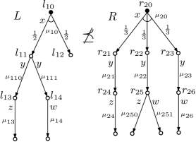
Figure 7: There is no reactive counterexample to $L\preceq R$.

Consider the LPTS $L$ and the reactive LPTS $R$ in Figure 7. The states along with the outgoing actions and distributions are labeled as in the figure. By similar arguments as made in the proof of Lemma 4, one can show that $\mu_{110}\not\sqsubseteq_{\preceq}\mu_{23}$, $\mu_{111}\not\sqsubseteq_{\preceq}\mu_{21}$ whereas $\mu_{110}\sqsubseteq_{\preceq}\mu_{21},\mu_{22}$ and $\mu_{111}\sqsubseteq_{\preceq}\mu_{22},\mu_{23}$. All these imply that $L\not\preceq R$. We are interested in a counterexample to show this.

Assume that a reactive LPTS $C$ exists which serves as a counterexample. Again, similar to the arguments made in the proof of Lemma 4, one can show that $C$ can only be a tree with exactly one transition $\mu_{0}$ labeled by $x$ from the initial state and for every state in $\text{{\em Supp}}(\mu_{0})$, there is at most one distribution labeled by $y$ (because $l_{11}$ has transitions on no other action). Furthermore, if any state in the support of this distribution has any transitions, all the transitions from all the states in the support will be labeled by the same action and that too, by either $z$ or $w$. Then, if $S_{y}$ is the set of states in $\text{{\em Supp}}(\mu_{0})$ with outgoing distributions (which should only be labeled by $y$) then $\mu_{0}(S_{y})\leq\frac{1}{2}$.

Now, we define a relation $V\subseteq S_{C}\times S_{2}$, where $S_{C}$ is the set of states of $C$, in a similar fashion. All the states in $C$ with no transitions are related to every state in $S_{2}$. The initial states are related. For every other state $c$, if it has a transition labeled by $z$ or $w$, $c$ is related to all the states having a transition on $z$ or $w$, respectively and if it is labeled by $y$, it is related to $r_{21}$ ($r_{23}$) and $r_{22}$ if the states in the support have transitions on $z$ ($w$) and to all three of $r_{21}$, $r_{22}$ and $r_{23}$ otherwise. One can similarly show that $V$ is a strong simulation implying $C\preceq R$. This contradicts the assumption that $C$ is a counterexample. ∎

Appendix 0.F Quotient is an Abstraction : $L\preceq L/\Pi$

It suffices to show that $R=\{(s,c)|s\in c,c\in\Pi\}$ is a strong simulation between $L$ and $L/\Pi$. Let $sRc$ and $s\xrightarrow{a}\mu$. As $s\in c$, there exists a transition, by Definition 8, $c\xrightarrow{a}\mu_{l}$ such that for every $c^{\prime}\in\Pi$, $\mu_{l}(c^{\prime})=\sum_{s^{\prime}\in c^{\prime}}\mu(s^{\prime})$. Let $S\subseteq S_{L}$. Now, $\mu(S)$

$$=\sum_{s^{\prime}\in S}\mu(s^{\prime})$$

$$=\sum_{c^{\prime}\in R(S)}\sum_{s^{\prime}\in c^{\prime}\cap S}\mu(s^{\prime})$$

$$\leq\sum_{c^{\prime}\in R(S)}\sum_{s^{\prime}\in c^{\prime}}\mu(s^{\prime})$$

$$=\sum_{c^{\prime}\in R(S)}\mu_{l}(c^{\prime})$$

$$=\mu_{l}(R(S))$$

As $S$ is arbitrary, this implies from Lemma 1 that $\mu\sqsubseteq_{R}\mu_{l}$. Note that $s^{0}_{L}R[s^{0}_{L}]$.

We conclude that $L\preceq L/\Pi$. ∎

Appendix 0.G Proof of Lemma 6

Let $s_{1}$, $\mu_{1}$ and $M$ be as in Section 4. Consider the first case where $R(s_{1})=\emptyset$. If $R_{\text{{\em old}}}(s_{1})=R_{M}(s_{1})$, it follows that there exists $s\in\text{{\em Supp}}(\mu_{1})$ with $R_{\text{{\em old}}}(s)\subset R_{M}(s)$. This can be easily proved by contradiction and we omit this proof. As $M(s)$ is split into $R_{\text{{\em old}}}(s)$ and the rest, the strategy results in a finer partition. Otherwise, $R_{\text{{\em old}}}(s_{1})$ is a strict subset of $R_{M}(s_{1})$ and as $R(s_{1})=\emptyset$, the strategy splits $M(s_{1})$ into $R_{\text{{\em old}}}(s_{1})$ and the rest which also results in a finer partition.

Now, consider the second case where $R(s_{1})\neq\emptyset$, $M(s_{1})=[s^{0}_{L}]_{\Pi}$ and $s^{0}_{L}\in R_{\text{{\em old}}}(s_{1})\setminus R(s_{1})$. It follows that $R_{\text{{\em old}}}(s_{1})\setminus R(s_{1})$ is a non-empty, proper subset of $R_{M}(s_{1})$ and hence, this also results in a finer partition. ∎

References

- [1] C. Baier. On Algorithmic Verification Methods for Probabilistic Systems. Habilitation thesis, Fakultät für Mathematik und Informatik, Univ. Mannheim, 1998.
- [2] C. Baier and J.-P. Katoen. Principles of Model Checking. MIT Press, Cambridge, MA, USA, 2008.
- [3] R. Chadha and M. Viswanathan. A Counterexample-Guided Abstraction-Refinement Framework for Markov Decision Processes. TOCL, 12(1):1–49, 2010.
- [4] S. Chaki, E. M. Clarke, N. Sinha, and P. Thati. Automated Assume-Guarantee Reasoning for Simulation Conformance. In CAV, vol. 3576 of LNCS, pp. 534–547. Springer-Verlag, 2005.
- [5] S. J. Chaki. A Counterexample Guided Abstraction Refinement Framework for Verifying Concurrent C Programs. PhD thesis, Carnegie Mellon University, 2005.
- [6] E. M. Clarke, O. Grumberg, S. Jha, Y. Lu, and H. Veith. Counterexample-Guided Abstraction Refinement. In CAV, vol. 1855 of LNCS, pp. 154–169, London, UK, 2000. Springer-Verlag.
- [7] E. M. Clarke, O. Grumberg, and D. A. Peled. Model Checking. MIT Press, Cambridge, MA, USA, 2000.
- [8] L. de Alfaro, T. A. Henzinger, and R. Jhala. Compositional Methods for Probabilistic Systems. In CONCUR, vol. 2154 of LNCS, pp. 351–365, London, UK, 2001. Springer-Verlag.
- [9] B. Dutertre and L. D. Moura. The Yices SMT Solver. Technical report, SRI International, 2006.
- [10] L. Feng, T. Han, M. Kwiatkowska, and D. Parker. Learning-based Compositional Verification for Synchronous Probabilistic Systems. In ATVA, vol. 6996 of LNCS, pp. 511–521, Heidelberg, 2011. Springer-Verlag.
- [11] L. Feng, M. Kwiatkowska, and D. Parker. Automated learning of probabilistic assumptions for compositional reasoning. In FASE, vol. 6603 of LNCS, pp. 2–17, Heidelberg, 2011. Springer-Verlag.
- [12] M. Gheorghiu Bobaru, C. S. Păsăreanu, and D. Giannakopoulou. Automated Assume-Guarantee Reasoning by Abstraction Refinement. In CAV, vol. 5123 of LNCS, pp. 135–148, Heidelberg, 2008. Springer-Verlag.
- [13] H. Hermanns, B. Wachter, and L. Zhang. Probabilistic CEGAR. In CAV, vol. 5123 of LNCS, pp. 162–175, Heidelberg, 2008. Springer-Verlag.
- [14] A. Komuravelli, C. S. Păsăreanu, and E. M. Clarke. Learning Probabilistic Systems from Tree Samples. In LICS, 2012. (to appear).
- [15] M. Kwiatkowska, G. Norman, and D. Parker. PRISM 4.0: Verification of Probabilistic Real-time Systems. In CAV, vol. 6806 of LNCS, pp. 585–591, Heidelberg, 2011. Springer-Verlag.
- [16] M. Kwiatkowska, G. Norman, D. Parker, and H. Qu. Assume-Guarantee Verification for Probabilistic Systems. In TACAS, vol. 6015 of LNCS, pp. 23–37, Heidelberg, 2010. Springer-Verlag.
- [17] R. Milner. An Algebraic Definition of Simulation between Programs. Technical report, Stanford University, 1971.
- [18] A. Pnueli. In Transition from Global to Modular Temporal Reasoning about Programs. In LMCS, vol. 13 of NATO ASI, pp. 123–144, New York, NY, 1985. Springer-Verlag.
- [19] C. S. Păsăreanu, D. Giannakopoulou, M. G. Bobaru, J. M. Cobleigh, and H. Barringer. Learning to Divide and Conquer: Applying the L* Algorithm to Automate Assume-Guarantee Reasoning. FMSD, 32(3):175–205, 2008.
- [20] R. Segala and N. Lynch. Probabilistic Simulations for Probabilistic Processes. Nordic J. of Computing, 2(2):250–273, 1995.
- [21] L. Zhang. Decision Algorithms for Probabilistic Simulations. PhD thesis, Universitä̈t des Saarlandes, 2008.