PACS: 42.50.-p, 03.67.-a, 03.65.Sq, 03.67.Dd

Abstract

We apply the Wigner function formalism to the study of two-photon polarization-momentum hyperentanglement generated in parametric down-conversion. It is shown that the consideration of a higher number of degrees of freedom is directly related to the extraction of additional uncorrelated sets of zeropoint modes at the source. We present a general expression for the description of the quantum correlations corresponding to the sixteen Bell base states, in terms of four beams whose amplitudes are correlated through the stochastic properties of the zeropoint field. A detailed analysis of the two experiments on complete Bell-state measurement included in [Walborn et al., Phys. Rev. A 68, 042313 (2003)] is made, emphasizing the role of the zeropoint field. Finally, we investigate the relationship between the zeropoint inputs at the source and the analysers, and the limits on optimal Bell-state measurement.

Keywords: Entanglement, Bell-state analysis, parametric down-conversion, Wigner representation, zeropoint field.

1 INTRODUCTION

In the last two decades, parametric down-conversion (PDC) assumed an important role for the practical implementation of the quantum theory of information, such as quantum cryptography [1], quantum dense coding [2] and teleportation [3]. The use of PDC as a source of entanglement involves the necessity of performing a complete Bell-state measurement (BSM), which is required in many quantum communication schemes. In this context, entangled photon pairs produced in PDC have been used for experiments on a partial Bell-state measurement [4], in which entanglement involves only one degree of freedom, and a complete Bell-state measurement, in which hyperentanglement (entanglement between two or more degrees of freedom) takes part [5]. More recently, these states have been used as an essential part of cluster states [6] which are of great value in the field of quantum computing [7].

The use of enlarged Hilbert spaces opened the door for a complete BSM using linear optics and single photon detectors, first by considering that one of the degrees of freedom was in a fixed quantum state [8], and encoding the information in the other. Further studies about the actual limits for BSM in these enlarged spaces have shown that, for two photons hyperentangled in $n$ degrees of freedom, the number of mutually distinguishable sets of Bell states is bounded above by $2^{n+1}$ [9]. More recently, it has been shown that at most $2^{n+1}-1$ classes out of $4^{n}$ hyper-Bell states can be distinguished with one copy of the input state, and that complete distinguishability is possible with two copies, within the class of devices obeying linear evolution and local measurement (LELM) [10]. In case the two photons are not brought together at the LELM apparatus the maximun number of distinguishable classes is $2^{n}$.

The Wigner representation of quantum optics provides an alternative to the standard Hilbert space formalism for the study of quantum information and for its practical implementation with PDC. In the Wigner representation within the Heisenberg picture (WRHP) the generation and propagation of PDC light is treated as in classical optics by taking into account the zeropoint field (ZPF) entering the crystal and the different optical devices placed between the source and the detectors. Finally, the vacuum fluctuations of the electromagnetic field are subtracted at the detectors [11, 12]. Hence, the peculiarities of the quantum world with respect to the image that classical physics offers are represented, in this context, by (i) the existence of a stochastic zeropoint field whose amplitudes are distributed according to a positive Wigner function, and (ii) the way in which the signal is separated from the zeropoint background in the detection process. These two features give rise to the typical counterintuitive results within the quantum domain.

In essence, manipulating entanglement is a common denominator in the different manifestations of quantum communication. In the WRHP, two-photon polarization entanglement is represented by two stochastic light beams, whose correlation properties arise from the coupling between two zeropoint beams (each containing two sets of uncorrelated zeropoint modes) and the laser beam at the crystal [12], following the classical Maxwell equations [13, 14]. On the other hand, entanglement manipulation involves the change in the correlation properties of the light beams when they are going through the different optical devices, and this is related to the way in which the vacuum modes are redistributed at the field amplitudes.

The WRHP description of the four polarization Bell base states was made in [15] along with the application of the formalism to experiments on quantum cryptography. In [16] partial Bell-state analysis was studied, and the fermionic behaviour of two photons described by the singlet state, when they reach a balanced beam-splitter, was explained using purely wave-mechanical arguments based on the Wigner representation. More recently, the WRHP formalism has been applied to the description of entanglement swapping using PDC light, and it has been shown that the generation of mode entanglement between two initially non interacting photons is related to the quadruple correlation properties of the electromagnetic field, through the stochastic properties of the vacuum [17]. These works emphasised the role of the zeropoint field in the generation and propagation of light in experimental implementations of quantum communication, including the existence of a relevant ZPF noise entering the idle channels of the analysers. Concretely, according to [15] the effects of eavesdropping attacks in the case of projective measurements are directly related to the inclusion of some fundamental noise, that also turns out to be fundamental to reproduce the quantum results. In this way, we can state that the zeropoint field carries the quantum information which is extracted at the source, and also introduces some fundamental noise at the idle channels of the analyzers. These two features of the zeropoint field are a common denominator in optical experiments on quantum information.

The standard Hilbert-space formulation of quantum optics considers vacuum fluctuations in an implicit way through the Heisenberg principle and the use of normal ordering for the calculation of photodetection probabilities. In contrast, the Wigner function offers the possibility of stating specifically what the role of vacuum fluctuations is in the generation and measurement of quantum information in quantum optical information processing using PDC. In this way, the motivation for this paper and further works comes from the following questions: What is the relationship between enlarging the Hilbert space and the zeropoint field activated at the source? What is the role of the zeropoint at the different stages of a BSM experiment? What is the relationship between the zeropoint modes entering the source, the ones activated at the idle channels of the analyzers, and the maximal information that can be generated in each experiment? Thus, there is considerable motivation for the application of the WRHP approach to the description of hyperentanglement and its application to complete Bell-state analysis, in order to investigate the role of the zeropoint field in this area.

The paper is organised as follows: In Section 2 we shall describe two-photon polarization-momentum hyperentanglement generated in PDC, by means of four correlated light beams. This description involves the consideration of eight uncorrelated sets of vacuum modes, distributed in four ZPF entering beams at the source. We shall obtain a compact expression for the description of the sixteen Bell base states in the WRHP, in terms of four two-by-two correlated beams. In Section 3 we shall apply this formalism to study the experiments proposed in reference [8] in which one of the degrees of freedom is in a fixed quantum state. We shall put the emphasis on the role of the zeropoint field at the different steps of each experiment, in order to make clear its relevant contribution to the signal fields arriving at the detectors. This analysis is important, not only for the theoretical aspects concerning optical experiments on quantum information, but also for its relation with optical tests of Bell’s inequalities, in which the vacuum field entering the idle channels of the analysers gives rise to enhancement [18, 19]. In Section 4 we shall demonstrate that the number of independent sets of zeropoint modes entering the source represents an upper bound to the maximum number of Bell states that can be distinguished in hyperentanglement-assisted Bell-state analysis. Also, we shall establish the relationship between the ZPF inputs at the source and the analysers, and the maximum number of distinguishable Bell-state classes, in LELM apparatus in which the left and right input channels are not brought together. Finally, in Section 5 we shall present the main conclusions of this work, and sketch further steps for future research. In order to a better understanding of the WRHP approach in this paper, we have included some fundamental ideas in Appendix A.

2 POLARIZATION-MOMENTUM HYPERENTANGLEMENT IN THE WRHP

Let us start by considering the following situation: a type-I two-crystal source is pumped by a laser beam. The first (second) crystal emits pairs of horizontal (vertical) polarized photons in superimposed emission cones. Because the photons are emitted on opposite sides of the cone, two sets of conjugated beams, $(a_{1},b_{2})$ and $(a_{2},b_{1})$, which are represented by wave vectors ${\bf k}_{a_{i}}$, ${\bf k}_{b_{i}}$ ($i=1,2)$, can be selected [20]. If the coherence volume of the laser contains the two-crystal interaction region, the quantum state corresponding to a photon pair is usually expressed, in a particle-like description, as:

$$|\Phi^{+}\rangle\otimes|\psi^{+}\rangle=\frac{1}{\sqrt{2}}[|H\rangle_{1}|H\rangle_{2}+|V\rangle_{1}|V\rangle_{2}]\otimes\frac{1}{\sqrt{2}}[|a\rangle_{1}|b\rangle_{2}+|b\rangle_{1}|a\rangle_{2}].$$ (1)

The state given by (1) is one of the sixteen base states corresponding to the two-photon hyperentanglement on polarization and momentum degrees of freedom, of the form $|\Pi\rangle\otimes|\eta\rangle$, where $|\Pi\rangle$ ($|\eta\rangle$) is the four-dimensional vector representing one of the polarization (momentum) Bell base states [8]:

$${\left|\Psi^{\pm}\right\rangle}=\frac{1}{\sqrt{2}}\left[{\left|H\right\rangle}_{1}{\left|V\right\rangle}_{2}\pm{\left|V\right\rangle}_{1}{\left|H\right\rangle}_{2}\right]\,\,\,;\,\,\,{\left|\Phi^{\pm}\right\rangle}=\frac{1}{\sqrt{2}}\left[{\left|H\right\rangle}_{1}{\left|H\right\rangle}_{2}\pm{\left|V\right\rangle}_{1}{\left|V\right\rangle}_{2}\right],$$ (2)

$${\left|\psi^{\pm}\right\rangle}=\frac{1}{\sqrt{2}}\left[{\left|a\right\rangle}_{1}{\left|b\right\rangle}_{2}\pm{\left|b\right\rangle}_{1}{\left|a\right\rangle}_{2}\right]\,\,\,;\,\,\,{\left|\phi^{\pm}\right\rangle}=\frac{1}{\sqrt{2}}\left[{\left|a\right\rangle}_{1}{\left|a\right\rangle}_{2}\pm{\left|b\right\rangle}_{1}{\left|b\right\rangle}_{2}\right].$$ (3)

The study of polarization-momentum hyperentanglement in the WRHP is based on the same ideas that were developed in references [11] and [12]. The key point in this case is that the selection of two sets of correlated beams, $(a_{1},b_{2})$ and $(a_{2},b_{1})$, implies the consideration of eight sets of vacuum modes which are “activated” at the crystal via the coupling with the laser beam (see fig.1). The set of representative modes, corresponding to the entering zeropoint beam of wave vector ${\bf k}_{x_{i}}$, is represented by the vacuum amplitudes:

$$\left\{\alpha_{x_{i},\lambda}\right\}\equiv\left\{\alpha_{{\bf k},\lambda};{\bf k}\in\left[{\bf k}\right]_{x_{i}}\right\}\,\,\,;\,\,\,x=a,b\,\,\,;\,\,\,\lambda=H,V\,\,;\,\,i=1,2.$$ (4)

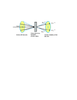
Figure 1: Sets of vacuum modes (on the left), which are “activated” and coupled with the laser inside the crystal. The correlation properties of the four beams (on the right) are related to the way in which the vacuum amplitudes are distributed in the field amplitudes. Hence, each of the sixteen Bell base states is characterized, in the WRHP approach, by a “particular” set of correlations.

In order to focus on the main points we shall first describe the generation of the beams concerning one of the sixteen states, the one corresponding to Eq. (1). The Hamiltonian corresponding to the electromagnetic field can be expressed in the following way:

$$H=H_{free}+H_{int}=\sum_{\lambda=H,V}\sum_{\bf k}\hbar\omega_{{\bf k},\lambda}\alpha_{{\bf k},\lambda}^{*}\alpha_{{\bf k},\lambda}$$

$${+\left(i\hbar g^{\prime}\frac{V}{2}\sum_{\begin{array}[]{l}{i,j=1}\\ {i\neq j}\end{array}}^{2}{\kern 1.0pt}\sum_{\lambda=H,V}\sum_{\begin{array}[]{l}{{\bf{k}}\in\left[{\bf{{\rm{\bf{k}}}}}\right]_{a_{i}}}\\ {{\bf{k}}^{\prime}\in\left[{\bf{{\rm{\bf{k}}}}}\right]_{b_{j}}}\end{array}}f\left({\bf{k}},{\bf{k^{\prime}}}\right)\exp\left(-i\omega_{p}t\right)\alpha_{{\bf{k}},\lambda}^{*}\alpha_{{\bf{k^{\prime}}},\lambda}^{*}+\rm c.c.\right),}$$ (5)

where the crucial difference between (5) and Eq. (1) of [12] is that we have made the change $V\rightarrow V/2$, in order to consider that the energy of the classical wave corresponding to the laser (with frequency $\omega_{p}$ and momentum ${\bf k}_{p}$), which is proportional to the squared amplitude, must be divided into four beams. On the other hand, $f\left({\bf{k}},{\bf{k^{\prime}}}\right)$ is a function which is different from zero only when the momentum matching condition is fulfilled, and $g^{\prime}$ is a constant related to the coupling parameter.

The evolution equation for $\alpha_{{\bf k},\lambda}$ is given by the Hamilton (canonical) equations, taking $\sqrt{\hbar}\alpha_{{\bf k},\lambda}$ as coordinates and $\sqrt{\hbar}\alpha^{*}_{{\bf k},\lambda}$ as canonical momenta. We have:

$$\dot{\alpha}_{{\bf k},\lambda}=-i\omega_{{\bf k},\lambda}\alpha_{{\bf k},\lambda}+g^{\prime}\frac{V}{2}\sum_{{\bf k}^{\prime}}f({\bf k},{\bf k}^{\prime})\exp(-i\omega_{p}t)\alpha_{{\bf k}^{\prime},\lambda}^{*},$$ (6)

where $\{{\bf k},\lambda\}$ represents any mode belonging to (4). The integration is performed to second order in the coupling constant ($g=g^{\prime}\Delta t$), from $t=-\Delta t$ to $t=0$, $\Delta t$ being the interaction time inside the two-crystal source. For $t>0$ there is a free evolution.

By substituting $\alpha_{{\bf k},H}(t)$ and $\alpha_{{\bf k},V}(t)$ in Eq. (A.1) we obtain the following four correlated beams leaving the crystal (for more details see [11, 12]):

$${\bf F}_{a_{1}}^{(+)}({\bf r},t)=F_{p}^{(+)}({\bf r},t;\{\alpha_{a_{1},H};\alpha^{*}_{b_{2},H}\}){\bf i}_{a_{1}}+F_{s}^{(+)}({\bf r},t;\{\alpha_{a_{1},V};\alpha^{*}_{b_{2},V}\}){\bf j}_{a_{1}},$$ (7)

$${\bf F}_{b_{2}}^{(+)}({\bf r},t)=F_{q}^{(+)}({\bf r},t;\{\alpha_{b_{2},H};\alpha^{*}_{a_{1},H}\}){\bf i}_{b_{2}}+F_{r}^{(+)}({\bf r},t;\{\alpha_{b_{2},V};\alpha^{*}_{a_{1},V}\}){\bf j}_{b_{2}},$$ (8)

$${\bf F}_{b_{1}}^{(+)}({\bf r},t)={F^{\prime}}_{p}^{(+)}({\bf r},t;\{\alpha_{b_{1},H};\alpha^{*}_{a_{2},H}\}){\bf i}_{b_{1}}+{F^{\prime}}_{s}^{(+)}({\bf r},t;\{\alpha_{b_{1},V};\alpha^{*}_{a_{2},V}\}){\bf j}_{b_{1}},$$ (9)

$${\bf F}_{a_{2}}^{(+)}({\bf r},t)={F^{\prime}}_{q}^{(+)}({\bf r},t;\{\alpha_{a_{2},H};\alpha^{*}_{b_{1},H}\}){\bf i}_{a_{2}}+{F^{\prime}}_{r}^{(+)}({\bf r},t;\{\alpha_{a_{2},V};\alpha^{*}_{b_{1},V}\}){\bf j}_{a_{2}},$$ (10)

where each polarization component is a linear transformation of the ZPF entering the nonlinear medium. We have included the sets of relevant zeropoint modes, for a better understanding of the correlation properties. For instance, $F_{p}^{(+)}$ is only correlated to $F_{q}^{(+)}$ because $\{\alpha_{a_{1},H}\}$ ($\{\alpha^{*}_{b_{2},H}\}$) is correlated to $\{\alpha^{*}_{a_{1},H}\}$ ($\{\alpha_{b_{2},H}\}$), as it can be seen from Eq. (A.4). The same reasoning applies to the correlations $F_{r}^{(+)}\leftrightarrow F_{s}^{(+)}$, ${F^{\prime}}_{p}^{(+)}\leftrightarrow{F^{\prime}}_{q}^{(+)}$, and ${F^{\prime}}_{r}^{(+)}\leftrightarrow{F^{\prime}}_{s}^{(+)}$. Hence, the beam ${\bf F}_{a_{1}}^{(+)}$ (${\bf F}_{b_{1}}^{(+)}$) is correlated to ${\bf F}_{b_{2}}^{(+)}$ (${\bf F}_{a_{2}}^{(+)}$), but there is no correlation between the two beams corresponding to each photon.

Taking ${\bf r}={\bf 0}$ at the center of the source, we have the cross-correlation:

$$\langle F_{p}^{(+)}({\bf 0},t)F_{q}^{(+)}({\bf 0},t^{\prime})\rangle=g\frac{V}{2}\nu(t^{\prime}-t),$$ (11)

where $\nu(t^{\prime}-t)$ vanishes when $|t^{\prime}-t|$ is greater than the correlation time between the beams ${\bf F}_{a_{1}}^{(+)}$ and ${\bf F}_{b_{2}}^{(+)}$ [13]. Similar expressions hold for $\langle{F^{\prime}}_{r}^{(+)}({\bf 0},t){F^{\prime}}_{s}^{(+)}({\bf 0},t^{\prime})\rangle$, $\langle F_{r}^{(+)}({\bf 0},t)F_{s}^{(+)}({\bf 0},t^{\prime})\rangle$, and $\langle{F^{\prime}}_{p}^{(+)}({\bf 0},t){F^{\prime}}_{q}^{(+)}({\bf 0},t^{\prime})\rangle$.

On the other hand, taking for instance the polarization amplitude $F_{p}^{(+)}$ at a point ${\bf r}$ and times $t$ and $t^{\prime}$, we have the autocorrelation:

$$\langle F_{p}^{(+)}({\bf r},t)F_{p}^{(-)}({\bf r},t^{\prime})\rangle-\langle[{\bf F}_{ZPF,a_{1}}^{(+)}({\bf r},t)\cdot{\bf i}_{a_{1}}][{\bf F}_{ZPF,a_{1}}^{(-)}({\bf r},t^{\prime})\cdot{\bf i}_{a_{1}}]\rangle$$

$$=\frac{g^{2}|V|^{2}}{4}\mu(t^{\prime}-t),$$ (12)

where ${\bf F}_{ZPF,a_{1}}^{(+)}$ is the zeropoint beam corresponding to mode $a_{1}$, and $\mu(t-t^{\prime})$ is a correlation function which goes to zero when $|t^{\prime}-t|$ is greater than the coherence time of PDC light. Similar expressions hold for $F_{s}^{(+)}$, $F_{q}^{(+)}$, $F_{r}^{(+)}$, and for the corresponding primed amplitudes.

2.1 The sixteen hyper-Bell states in the WRHP

The four beams given in Eqs. (7) to (10) are correlated through the ZPF entering the two-crystal source, which is “amplified” via the activation of the eight sets of vacuum modes $\{{\bf k}_{x_{i},\lambda}\,\,(x=a,b;i=1,2;\lambda=H,V)\}$. The beams ${\bf F}_{a_{1}}^{(+)}$ and ${\bf F}_{b_{1}}^{(+)}$ can be locally manipulated, allowing for the possibility of distributing the vacuum amplitudes in sixteen different ways, each corresponding to the generation of a concrete Bell base state. Hence, the possibility of performing superdense coding is explained in the WRHP framework through the change of the correlation properties of the light beams (represented by the four nonvanishing correlations $p\leftrightarrow q$ and $r\leftrightarrow s$) when the two uncorrelated beams corresponding to one photon are modified via local manipulations. Such correlations have their origin in the crystal, where the zeropoint modes are coupled with the laser field, and the information is carried by the amplified vacuum fluctuations.

Now let us characterize the correlation properties of the sixteen Bell base states. For this purpose the description of the four polarization Bell-states, in terms of two-parametrized two correlated beams, will be considered here [16]. For the sake of simplicity, from now on in this section we shall discard the dependence on position and time. We have:

$${\bf F}_{x_{1}}^{(+)}=\left\{[F_{s}^{(+)}{\rm cos}\beta-F_{p}^{(+)}{\rm sin}\beta]{\bf i}_{x_{1}}+{\rm e}^{i\kappa}[F_{s}^{(+)}{\rm sin}\beta+F_{p}^{(+)}{\rm cos}\beta]{\bf j}_{x_{1}}\right\}{\rm e}^{i\varphi_{1}},$$ (13)

$${\bf F}_{y_{1}}^{(+)}=\left\{[{F^{\prime}}_{s}^{(+)}{\rm cos}\beta-{F^{\prime}}_{p}^{(+)}{\rm sin}\beta]{\bf i}_{y_{1}}+{\rm e}^{i\kappa}[{F^{\prime}}_{s}^{(+)}{\rm sin}\beta+{F^{\prime}}_{p}^{(+)}{\rm cos}\beta]{\bf j}_{y_{1}}\right\}{\rm e}^{i\varphi_{2}},$$ (14)

$${\bf F}_{a_{2}}^{(+)}={F^{\prime}}_{q}^{(+)}{\bf i}_{a_{2}}+{F^{\prime}}_{r}^{(+)}{\bf j}_{a_{2}},$$ (15)

$${\bf F}_{b_{2}}^{(+)}=F_{q}^{(+)}{\bf i}_{b_{2}}+F_{r}^{(+)}{\bf j}_{b_{2}},$$ (16)

where ${\bf F}_{x_{1}}^{(+)}$ (${\bf F}_{y_{1}}^{(+)}$) is correlated to ${\bf F}_{b_{2}}^{(+)}$ (${\bf F}_{a_{2}}^{(+)}$).

Eqs. (13) to (16) correspond to the description, in the WRHP, of the sixteen Bell base states corresponding to polarization-momentum hyperentanglement of two photons. The essential point is that quantum correlations are described in terms of four two-by-two correlated beams through the eight sets of independent zeropoint amplitudes entering the nonlinear source.

The transformations concerning polarization are represented by two parameters, $\beta$ and $\kappa$, which represent the action of a polarization rotator and a wave retarder, respectively, on beams corresponding to photon “$1$”. In this way, the combination $\beta=0$, $\kappa=0$ ($\beta=0$, $\kappa=\pi$) corresponds to the description of the polarization state $|\Psi^{+}\rangle$ ($|\Psi^{-}\rangle$). In both cases the non-null correlations correspond to different polarization components, the only difference being the minus sign that appears in $|\Psi^{-}\rangle$. On the other hand, the case $\beta=\mp\pi/2$ and $\kappa=\pi$ ($\beta=-\pi/2$, $\kappa=0$) corresponds to the description of $\mp|\Phi^{+}\rangle$ ($|\Phi^{-}\rangle$), where the horizontal (vertical) component of a beam is correlated with the horizontal (vertical) component of the conjugated one [16].

On the other hand, momentum is represented by two couples of parameters, $(x,y)$ and $(\varphi_{1},\varphi_{2})$, such that:

• The combination $(x,y)=(a,b)$ ($(x,y)=(b,a)$) and $\varphi_{1}=\varphi_{2}=0$ corresponds to the state $|\psi^{+}\rangle$ ($|\phi^{+}\rangle$).

• The situation in which $(x,y)=(a,b)$, $\varphi_{1}=0$ and $\varphi_{2}=\pi$, corresponds to $|\psi^{-}\rangle$.

• Finally, in the case $(x,y)=(b,a)$, $\varphi_{1}=\pi$ and $\varphi_{2}=0$, we have the description of $|\phi^{-}\rangle$.

Because of the fact that multiplying a given Bell state by a phase factor is irrelevant, it can be easily seen that there are four dichotomic parameters giving rise to the sixteen Bell base states. For instance, the parameters $\beta=(0,-\pi/2)$ and $\kappa=(0,\pi)$ define the polarization Bell-state, and $[x,y]=[(a,b),(b,a)]$ and $[\varphi_{1},\varphi_{2}]=[(0,0),(0,\pi)]$ the momentum Bell-state. These parameters can be changed locally, and this property is of interest in connection to dense coding and superdense coding [8, 9].

3 COMPLETE BSM IN THE WRHP

In this section we shall apply the Wigner formalism for hyperentanglement to the description of a complete BSM of the four Bell states, by considering that one of the two degrees of freedom is in a fixed state: (i) First, we shall consider the experimental setup shown in Fig. 2 of reference [8], in which the momentum degrees of freedom are used as the ancilla, in order to encode information in polarization Bell states; (ii) in the second experiment (Fig. 3 of [8]), the polarization state is fixed, and the four momentum Bell-states can be distinguished.

Both setups correspond to a broad class of LELM devices, in which the modes corresponding to the input photons are not brought together in the apparatus. In this case, it has been demonstrated that there are at most $2^{n}$ distinguishable classes of Bell states [10]. As we are considering experiments in which one of the degrees of freedom is in a fixed state, each of the $2^{2}=4$ distinguishable classes of Bell states will just correspond to one of the four Bell states of the other degree of freedom.

In order to focus on the role of the zeropoint field, we shall describe the different steps of the experiments. The values of the field amplitudes at the detectors are usually computed by propagating them through the optical devices from the source to the detectors. In these experiments an identical distance separating the source from the respective optical devices and detectors will be considered, so that the contribution of the related phase shift in Eq. (16) of [12] will be discarded in the calculation of the probabilities. For simplicity, we shall focus on the ideal situation $t=t^{\prime}$, so that we can discard the dependence on position and time.

3.1 Discrimination of the polarization Bell-states

The hyperentangled-Bell-state analyser includes two polarizing beam-splitters (PBS) which transmit (reflect) the vertical (horizontal) polarization, and switch modes (remain in the same mode), in order to perform a controlled-NOT (CNOT) logic operation between the polarization (control) and spatial (target) degrees of freedom. Each outgoing beam passes through a polarization analyzer (PA) in the $\pm 45^{\circ}$ basis, consisting of a half-wave plate, a PBS, and two detectors. The vacuum zeropoint field at the idle channels of the analyzers is represented in Fig. 2, this being an important ingredient of our approach, as we shall see later.

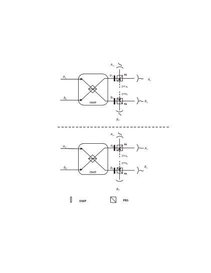
Figure 2: Polarization-momentum hyperentanglement analyzer using a fixed entangled state in momentum. The consideration of the zeropoint field at the idle channels of the analyzers is a key point in the Wigner approach.

By considering $(x,y)=(a,b)$ and $\varphi_{1}=\varphi_{2}=0$ in Eqs. (13) to (16), we obtain four correlated beams which describe one of the four states: $|\Psi^{\pm}\rangle\otimes|\psi^{+}\rangle$ and $|\Phi^{\pm}\rangle\otimes|\psi^{+}\rangle$, depending on the value of $\beta$ and $\kappa$. The action of CNOT gates is represented by the following output beams:

$${\bf{F^{\prime}}}_{a_{1}}^{(+)}=i[F_{s}^{(+)}{\rm cos}\beta-F_{p}^{(+)}{\rm sin}\beta]{\bf{i}}_{a_{1}}+{\rm e}^{i\kappa}[{F^{\prime}}_{s}^{(+)}{\rm sin}\beta+{F^{\prime}}_{p}^{(+)}{\rm cos}\beta]{\bf{j}}_{a_{1}},$$ (17)

$${\bf{F^{\prime}}}_{b_{1}}^{(+)}=i[{F^{\prime}}_{s}^{(+)}{\rm cos}\beta-{F^{\prime}}_{p}^{(+)}{\rm sin}\beta]{\bf{i}}_{b_{1}}+{\rm e}^{i\kappa}[F_{s}^{(+)}{\rm sin}\beta+F_{p}^{(+)}{\rm cos}\beta]{\bf{j}}_{b_{1}},$$ (18)

$${\bf{F^{\prime}}}_{a_{2}}^{(+)}=i{F^{\prime}}_{q}^{(+)}{\bf{i}}_{a_{2}}+F_{r}^{(+)}{\bf{j}}_{a_{2}},$$ (19)

$${\bf{F^{\prime}}}_{b_{2}}^{(+)}=iF_{q}^{(+)}{\bf i}_{b_{2}}+{F^{\prime}}_{r}^{(+)}{\bf j}_{b_{2}},$$ (20)

where we have considered the imaginary unit in order to account for the reflection at the PBS, in contrast to the equation (3) of reference [8], in which there is no phase shift associated to the reflection.

A quick look at Eqs. (17) to (20) shows that, in the case $\beta=0$, the nonzero correlations are those concerning amplitudes related to orthogonal polarizations of beams $a_{1}$ and $a_{2}$, or $b_{1}$ and $b_{2}$. This is consistent with the transformation $|\Psi^{\pm}\rangle|\psi^{+}\rangle\rightarrow|\Psi^{\pm}\rangle|\phi^{+}\rangle$ (see Eq. (4) of [8]). In contrast, in the case $\beta=\pm\pi/2$ there is no change in the correlation properties of the light beams. These properties justify that the momentum state $|\psi^{+}\rangle$ can be used to discriminate between the four polarization Bell states. It is noteworthy that there is no additional zeropoint amplitudes entering the PBSs at the CNOT gates (see Fig. 2), so that the PBSs mark the momentum state due to the consideration of the eight sets of independent zeropoint modes at the two-crystal source, and their subsequent redistribution in the beams’ amplitudes.

Now, taking into account the action of the half-wave plate -HWP$@45^{\circ}$-, and that the polarization analyzers are oriented at $45^{\circ}$, the polarizing beam-splitters will reflect (transmit) the component of the field along the unit vector ${\bf{i}}$ (${\bf j}$), which is oriented at $+45^{\circ}$ ($-45^{\circ}$) with respect to the horizontal direction. In order to express the field amplitudes at the detectors, we must add the corresponding zero-point component that enters through the free channel of each PBS. After some easy algebra, we obtain the following compact expression for the four field amplitudes at the detectors, concerning the paths $a_{1}$ and $b_{1}$:

$${\bf F}_{X_{1\pm}}^{(+)}=\frac{i^{n_{1\pm}}}{\sqrt{2}}\left\{i[\widetilde{F}_{s,X}^{(+)}{\rm cos}\beta-\widetilde{F}_{p,X}^{(+)}{\rm sin}\beta]\pm{\rm e}^{i\kappa}[\check{F}_{s,X}^{(+)}{\rm sin}\beta+\check{F}_{p,X}^{(+)}\cos\beta]\right\}{\bf{u}}_{\pm}$$

$$+i^{m_{1\pm}}[{\bf{F}}_{ZPFX_{1}}^{(+)}\cdot{\bf{u}}_{\mp}]{\bf{u}}_{\mp},$$ (21)

and for the paths $a_{2}$ and $b_{2}$

$${\bf{F}}_{Y_{2\pm}}^{(+)}=\frac{i^{n_{2\pm}}}{\sqrt{2}}[i\check{F}_{q,Y}^{(+)}\pm\widetilde{F}_{r,Y}^{(+)}]{\bf{u}}_{\pm}+i^{m_{2\pm}}[{\bf{F}}_{ZPFY_{2}}^{(+)}\cdot{\bf{u}}_{\mp}]{\bf{u}}_{\mp},$$ (22)

where: $X,Y=A$ or $B$; ${\bf{u}}_{+}\equiv\bf{i}$, ${\bf{u}}_{-}\equiv\bf{j}$, and $n_{i+}=1$, $n_{i-}=0$, $m_{i+}=0$, $m_{i-}=1$, for $i=1,2$. Also we have defined the amplitudes $\widetilde{F}_{v,Z}^{(+)}$ and $\check{F}_{v,Z}^{(+)}$ ($v=p,q,r,s$; $Z=X,Y$), where $\widetilde{F}_{v,Z}^{(+)}=F_{v}^{(+)}$ in the case $Z=A$, and $\widetilde{F}_{v,Z}^{(+)}={F^{\prime}}_{v}^{(+)}$ stands for $Z=B$. In contrast, $\check{F}_{v,Z}^{(+)}={F^{\prime}}_{v}^{(+)}$ in the case $Z=B$, and $\check{F}_{v,Z}^{(+)}={F}_{v}^{(+)}$ stands for $Z=A$.

In order to calculate the joint detection probabilities we shall use Eq. (A.7) along with the correlation properties given in Eq. (11). We shall take into account that the ZPF inputs at the PBSs are uncorrelated with the signals and with each other. After some easy calculations, we obtain the following general expression for the joint detection probability:

$$\frac{P_{X_{1\pm},Y_{2\pm}}}{k_{X_{1\pm}}k_{Y_{2\pm}}}=\frac{1}{4}\left|[-i^{2}\langle\check{F}_{q,Y}^{(+)}\widetilde{F}_{p,X}^{(+)}\rangle+(\pm)_{1}(\pm)_{2}{\rm e}^{i\kappa}\langle\widetilde{F}_{r,Y}^{(+)}\check{F}_{s,X}^{(+)}\rangle]{\rm sin}\beta\right.$$

$$\left.+i[(\pm)_{2}\langle\widetilde{F}_{r,Y}^{(+)}\widetilde{F}_{s,X}^{(+)}\rangle+(\pm)_{1}\langle\check{F}_{q,Y}^{(+)}\check{F}_{p,X}^{(+)}\rangle]{\rm cos}\beta\right|^{2},$$ (23)

where $k_{X_{1\pm}}$, $k_{Y_{2\pm}}$, are constants which are related to the effective efficiency of the detection process. Let us now consider the following cases:

• Case I ($\beta=0$) corresponds to the states $|\Psi^{\pm}\rangle\otimes|\psi^{+}\rangle$. From (23) it can be easily shown that for $\kappa=0$ ($\kappa=\pi$), which corresponds to the polarization state $|\Psi^{+}\rangle$ ($|\Psi^{-}\rangle$), only the four probabilities $P_{A_{1+},A_{2+}}$, $P_{B_{1+},B_{2+}}$, $P_{A_{1-},A_{2-}}$, $P_{B_{1-},B_{2-}}$ ($P_{A_{1+},A_{2-}}$, $P_{B_{1+},B_{2-}}$, $P_{A_{1-},A_{2+}}$, $P_{B_{1-},B_{2+}}$) are different from zero.

• Case II ($\beta=\pm\pi/2$) corresponds to the states $|\Phi^{\pm}\rangle\otimes|\psi^{+}\rangle$. In this case, from (23) it is shown that for $\kappa=0$ ($\kappa=\pi$), which corresponds to the polarization state $|\Phi^{-}\rangle$ ($|\Phi^{+}\rangle$), only the four probabilities $P_{A_{1+},B_{2+}}$, $P_{B_{1+},A_{2+}}$, $P_{A_{1-},B_{2-}}$, $P_{B_{1-},A_{2-}}$ ($P_{A_{1+},B_{2-}}$, $P_{B_{1+},A_{2-}}$, $P_{A_{1-},B_{2+}}$, $P_{B_{1-},A_{2+}}$) are nonzero.

Hence, the detector signatures allow to distinguish between the polarization Bell states. The discrepancy with Walborn’s Table I in ref. [8], with respect to the states $|\Phi^{-}\rangle$ and $|\Phi^{+}\rangle$, is due to the consideration of the complex factor $i$ for the reflected amplitudes at the CNOT gates [21]. For this reason, the corresponding joint probabilities for these two states are exchanged with respect to the work of Walborn et al.

3.2 Discrimination of the momentum Bell-states

The experimental setup is shown in Fig. 3. Two half-wave plates (HWP), which are aligned at $45^{\circ}$ in modes $b_{1}$ and $b_{2}$, perform the CNOT operation. The BSs are balanced nonpolarizing beam splitters [8]. In this case, the polarization degrees of freedom are used as ancilla, so that the polarization state is fixed, and corresponds to $|\Psi^{+}\rangle$. In the Wigner formalism, by putting $\kappa=\beta=0$ in Eqs. (13) to (16), we obtain the following four beams in order to compactly describe the four states $|\Psi^{+}\rangle\otimes|\psi^{\pm}\rangle$ and $|\Psi^{+}\rangle\otimes|\phi^{\pm}\rangle$:

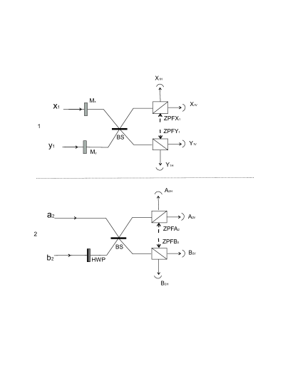
Figure 3: Hyperentangled-Bell-state analyzer using a fixed entangled state in polarization. We have represented two optical devices, $M_{x}$ and $M_{y}$, in order to account for the two possibilities, depending on the value of $x$ and $y$. The zeropoint field at the idle channels of the analyzers is represented by four beams.

$${\bf F}_{x_{1}}^{(+)}=[F_{s}^{(+)}{\bf i}_{x_{1}}+F_{p}^{(+)}{\bf j}_{x_{1}}]{\rm e}^{i\varphi_{1}},$$ (24)

$${\bf F}_{y_{1}}^{(+)}=[{F^{\prime}}_{s}^{(+)}{\bf i}_{y_{1}}+{F^{\prime}}_{p}^{(+)}{\bf j}_{y_{1}}]{\rm e}^{i\varphi_{2}},$$ (25)

$${\bf F}_{a_{2}}^{(+)}={F^{\prime}}_{q}^{(+)}{\bf i}_{a_{2}}+{F^{\prime}}_{r}^{(+)}{\bf j}_{a_{2}}$$ (26)

$${\bf F}_{b_{2}}^{(+)}=F_{q}^{(+)}{\bf i}_{b_{2}}+F_{r}^{(+)}{\bf j}_{b_{2}}.$$ (27)

Now, we define the matrices $\hat{M_{x}}$ and $\hat{M_{y}}$: in the case $x=a$, $y=b$, $\hat{M_{x}}=\hat{I}$ (identity matrix) and $\hat{M_{y}}=\hat{M}_{HWP}$; on the other hand, if $x=b$, $y=a$, then $\hat{M_{x}}=\hat{M}_{HWP}$ and $\hat{M_{y}}=\hat{I}$. In this way, the beams entering the BSs are

$${\bf{F^{\prime}}}_{x_{1}}^{(+)}=\hat{M_{x}}{\bf{F}}_{x_{1}}^{(+)}\,\,\,\,;\,\,\,\,{\bf{F^{\prime}}}_{y_{1}}^{(+)}=\hat{M_{y}}{\bf{F}}_{y_{1}}^{(+)},$$ (28)

$${\bf{F^{\prime}}}_{a_{2}}^{(+)}={\bf{F}}_{a_{2}}^{(+)}\,\,\,\,;\,\,\,\,{\bf{F^{\prime}}}_{b_{2}}^{(+)}=\hat{M}_{HWP}{\bf{F}}_{b_{2}}^{(+)}=F_{r}^{(+)}{\bf i}_{b_{2}}+F_{q}^{(+)}{\bf j}_{b_{2}}.$$ (29)

From Eqs. (28) and (29) it can be easily seen that, for $x=a$, $y=b$ ($x=b$, $y=a$), the only non-null cross-correlations are those concerning the same polarization (orthogonal polarizations). For this reason, the CNOT operation marks the polarization state. This operation does not introduce additional zeropoint fluctuations, because the HWPs do not activate zeropoint modes. Finally, the BSs transform the beams given in Eqs. (28) and (29) without the consideration of additional zeropoint modes, because there is no idle channel at the BSs.

Finally, if we consider the zeropoint amplitudes at the idle channels of the PBSs (see Fig. 3), the field amplitudes at the detectors $X_{1H}$, $X_{1V}$, $Y_{1H}$ and $Y_{1V}$ can be expressed by the following compact expression:

$$F_{Z_{1\lambda}}^{(+)}=\frac{i^{n_{\lambda}}}{\sqrt{2}}\left\{i^{m_{1}(Z)}[\hat{M_{x}}{\bf{F}}_{x_{1}}^{(+)}]+i^{m_{2}(Z)}[\hat{M_{y}}{\bf{F}}_{y_{1}}^{(+)}]\right\}\cdot{\bf u}_{\lambda}+F_{vac,Z_{1\lambda}}^{(+)},$$ (30)

where: $Z=X,Y$, $\lambda=H,V$; ${\bf{u}}_{H}\equiv\bf{i}$, ${\bf{u}}_{V}\equiv\bf{j}$; $n_{H}=1$, $n_{V}=0$; $m_{1}(X)=1$, $m_{1}(Y)=0$; $m_{2}(X)=0$, $m_{2}(Y)=1$.

In the same way, we have the following expression for the field amplitudes at the detectors $A_{2H}$, $A_{2V}$, $B_{2H}$ and $B_{2V}$:

$$F_{V_{2\lambda^{\prime}}}^{(+)}=\frac{i^{n_{\lambda^{\prime}}}}{\sqrt{2}}\left\{i^{m_{1}(V)}{\bf{F}}_{a_{2}}^{(+)}+i^{m_{2}(V)}[\hat{M}_{HWP}{\bf{F}}_{b_{2}}^{(+)}]\right\}\cdot{\bf u}_{\lambda^{\prime}}+F_{vac,V_{2\lambda^{\prime}}}^{(+)},$$ (31)

where: $V=A,B$, $\lambda^{\prime}=H,V$; $m_{1}(A)=1$, $m_{1}(B)=0$; $m_{2}(A)=0$, $m_{2}(B)=1$.

Now, using Eqs. (11) and (A.7), and taking into account that the ZPF inputs at the PBSs are uncorrelated with the signals and with each other, we shall consider the following cases:

• Case I ($x=a$, $y=b$) corresponds to the states $|\Psi^{+}\rangle\otimes|\psi^{\pm}\rangle$. After some easy algebra, we obtain:

  $$\begin{array}[]{l}\frac{P_{A_{1H},A_{2H}}}{k_{A_{1H}}k_{A_{2H}}}=\frac{P_{B_{1H},B_{2H}}}{k_{B_{1H}}k_{B_{2H}}}=\frac{P_{A_{1V},A_{2V}}}{k_{A_{1V}}k_{A_{2V}}}=\frac{P_{B_{1V},B_{2V}}}{k_{B_{1V}}k_{B_{2V}}}=\frac{g^{2}|V|^{2}|\nu(0)|^{2}}{16}\left|e^{i\varphi_{1}}+e^{i\varphi_{2}}\right|^{2},\end{array}$$ (32)

  and

  $$\begin{array}[]{l}\frac{P_{A_{1H},B_{2H}}}{k_{A_{1H}}k_{B_{2H}}}=\frac{P_{B_{1H},A_{2H}}}{k_{B_{1H}}k_{A_{2H}}}=\frac{P_{A_{1V},B_{2V}}}{k_{A_{1V}}k_{B_{2V}}}=\frac{P_{B_{1V},A_{2V}}}{k_{B_{1V}}k_{A_{2V}}}=\frac{g^{2}|V|^{2}|\nu(0)|^{2}}{16}\left|e^{i\varphi_{1}}-e^{i\varphi_{2}}\right|^{2}.\end{array}$$ (33)

  From Eqs. (32) and (33) it can be seen that, in the case $\varphi_{1}=\varphi_{2}=0$ ($\varphi_{1}=0$, $\varphi_{2}=\pi$), which corresponds to the momentum state $|\psi^{+}\rangle$ ($|\psi^{-}\rangle$), only the four probabilities in Eq. (32) (Eq. (33)) are nonzero.

• Case II ($x=b$, $y=a$) corresponds to the states $|\Psi^{+}\rangle\otimes|\phi^{\pm}\rangle$. In this case, we obtain:

  $$\begin{array}[]{l}\frac{P_{A_{1H},A_{2V}}}{k_{A_{1H}}k_{A_{2V}}}=\frac{P_{A_{1V},A_{2H}}}{k_{A_{1V}}k_{A_{2H}}}=\frac{P_{B_{1H},B_{2V}}}{k_{B_{1H}}k_{B_{2V}}}=\frac{P_{B_{1V},B_{2H}}}{k_{B_{1V}}k_{B_{2H}}}=\frac{g^{2}|V|^{2}|\nu(0)|^{2}}{16}\left|e^{i\varphi_{1}}-e^{i\varphi_{2}}\right|^{2}.\end{array}$$ (34)

  The above probabilities are non-null only in the case $\varphi_{1}=\pi$, $\varphi_{2}=0$ (or viceversa), i.e. the WRHP description of the momentum state $|\phi^{-}\rangle$. On the other hand:

  $$\begin{array}[]{l}\frac{P_{A_{1H},B_{2V}}}{k_{A_{1H}}k_{B_{2V}}}=\frac{P_{A_{1V},B_{2H}}}{k_{A_{1V}}k_{B_{2H}}}=\frac{P_{B_{1H},A_{2V}}}{k_{B_{1H}}k_{A_{2V}}}=\frac{P_{B_{1V},A_{2H}}}{k_{B_{1V}}k_{A_{2H}}}=\frac{g^{2}|V|^{2}|\nu(0)|^{2}}{16}\left|e^{i\varphi_{1}}+e^{i\varphi_{2}}\right|^{2}.\end{array}$$ (35)

  From Eq. (35), the corresponding probabilities are non-null only in the case $\varphi_{1}=\varphi_{2}=0$, i.e. the situation corresponding to the momentum state $|\phi^{+}\rangle$.

There is a discrepancy with Walborn’s Table II in ref. [8], with respect to the states $|\phi^{-}\rangle$ and $|\phi^{+}\rangle$, which is due to the consideration of the complex factor $i$ for the reflected amplitudes at the BSs [21]. Then, the corresponding joint probabilities for these two states are exchanged with respect to the work of Walborn et al.

4 ZPF AND THE LIMITS ON OPTIMAL BSM

Let us consider the following situation: two photons entangled in $n$ dichotomic degrees of freedom enter a LELM apparatus via separate spatial channels, designated $L$ and $R$. Each photon contains $2^{n}$ modes, and a unitary matrix transforms the $2^{n+1}$ input modes to $2^{n+1}$ output modes to the detectors. In [10] it is demonstrated that: (i) A single detector click cannot discriminate between any of the Bell states, so that the $2^{n+1}$ possibilities for the second detector event form a simple upper bound on distinguishable Bell-state classes using LELM devices; (ii) There can be at most $2^{n+1}-1$ distinguishable classes of hyper-Bell states for two bosons. This number is reduced to $2^{n}$ in the case that the left and right channels are not brought together in the apparatus. The experiments described in Sec. 3 are just an example of this situation in the case of photons, for $n=2$. This section is divided in two parts: (1) First, we shall investigate the relationship between the statement (i) and the zeropoint field inputs when optical experiments using parametric down conversion are considered; (2)  We shall study the relationship between the number of vacuum inputs at the source and the analysers, and the maximum number of distinguishable classes, $2^{n}$, in the kind of experiments as the ones described in Sec. 3.

1. Given an optical n-qubit state, the maximum number of mutually distinguishable sets of Bell states is bounded above by $2^{n+1}$ [9, 10]. The demonstration of this point in the Hilbert space is based on a particle-like description, which contrasts to the image in the WRHP formalism. For instance, in [16] it was stressed that two-photon entanglement in only one degree of freedom implies the consideration of four independent sets of zeropoint modes at the source, which are “activated” through a coupling with the laser inside the crystal. In this paper, the generation of polarization-momentum hyperentanglement is represented via the consideration of eight sets of independent vacuum modes, which are amplified at the two-crystal source. Hence, hyperentanglement, i.e. entanglement in Hilbert spaces of higher dimensions is closely related to the inclusion of more sets of vacuum modes entering the source. With an increasing number of vacuum inputs, the possibility of extracting more information from the zeropoint field also increases. As we shall demonstrate below, for a given $n$, the maximal distinguishability in a Bell-like experiment is bounded by the number of independent vacuum sets of modes which are extracted at the source, being this number equal to $2^{n+1}$. In order to prove this statement, we shall consider the following lemmas:

   Lemma I: For a two-photon n-qubit state generated via PDC, the number of independent sets of zeropoint modes which are necessary for the generation of entanglement, is just $2^{n+1}$.

   Proof: By considering the situation described in this paper, in which $n=2$, the interaction Hamiltonian given in Eq. (5) gives rise to linear evolution equations for the amplitudes $\alpha_{{\bf k},\lambda}$ [see Eq. (6)]. Hence, the $2^{n+1}$ sets of field amplitudes outgoing the crystal are generated from an identical number of independent sets of ZPF amplitudes entering the nonlinear source, which are “amplified” via the coupling with the laser beam. This result is also true for $n=1$, as it has been demonstrated elsewhere [12, 16]. For $n>2$, the interaction Hamiltonian is also quadratic, which implies that the evolution equations for the vacuum amplitudes are linear. Hence, this result is valid for any $n\geq 1$.

   Lemma II: The propagation of the $2^{n+1}$ sets of field amplitudes outgoing the crystal through a LELM device gives rise to $2^{n+1}$ output amplitudes to the detectors. Each of them will include, at least, the $2^{n+1}$ sets of input ZPF amplitudes at the source.

   Proof: Given the fact that linear mode transformations lead to Bogoliubov transformations of the mode operators, which are generated via quadratic Hamiltonians [22], the total set of unitary transformations, including the generation of PDC light at the crystal and the action of linear optical devices between the nonlinear source and the detectors, are represented by quadratic Hamiltonians in mode operators, which give rise to linear equations (see Fig. 4). When passing to the Wigner representation, in which the destruction (creation) operator $\hat{a}_{{\bf k},\lambda}$ ($\hat{a}^{\dagger}_{{\bf k},\lambda}$) is substituted by a complex amplitude $\alpha_{{\bf k},\lambda}$ ($\alpha_{{\bf k},\lambda}^{*}$), each of the $2^{n+1}$ output field amplitudes at the detectors will include, generally, the $2^{n+1}$ sets of field amplitudes outgoing the crystal, and so the $2^{n+1}$ input ZPF amplitudes at the nonlinear source (see Lemma I).

   Lemma III: The $2^{n+1}$ possibilities for the second detection event, which constitutes a simple upper bound on distinguishable Bell-state classes from LELM devices, is just the number of the input ZPF sets of modes at the source.

   Proof: This result follows from lemmas $I$ and $II$.

   Hence, the upper bound of $2^{n+1}$, which limits the optimality of any Bell-state analysis, coincides with the number of relevant ZPF modes at the source. This key point represents the relationship between the information that can be effectively measured in an experiment and the ZPF inputs at the source. In other words, the number of relevant sets of zeropoint modes at the source represents a limit on optimal Bell-state analysis in the enlarged Hilbert space.

   From [10], it is well known that a single detector event cannot discriminate any of the Bell base states. Let us consider that a PBS is placed at each of the beams (13) to (16) in order to measure the single and joint detection probabilities, following a setup similar to Fig. 1 of Ref. [15], and taking into account the vacuum inputs at the idle channels of the PBSs. Using the autocorrelation properties of the light field given in Eq. (12), the expression (A.5) for the single detection probability, and the field amplitudes at the detectors, it can be easily demonstrated that the single detection probabilities are identical, and independent of the parameters $\beta$, $\kappa$, $(x,y)$ and $(\varphi_{1},\varphi_{2})$. The same reasoning holds for the experiments developed in Sec.3, by using the field amplitudes at the detectors given in Eqs. (21) and (22) [(30) and (31)] for the first (second) experiment.

   

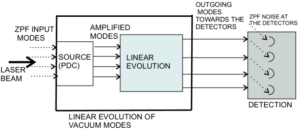
   Figure 4: The ZPF inputs at the non linear source are amplified and propagate through linear devices. The total set of transformations are represented by a quadratic Hamiltonian which gives rise to linear evolution equations. The total number of modes outgoing towards the detectors is equal to the entering ZPF modes at the crystal, which are amplified via the coupling with the laser beam. We have also represented the ZPF inputs at the detectors.

2. The noise entering the idle channels of the analyzers limits the optimality of the Bell-state analysis, and this idea is worthy of consideration. In Section 3 we have applied the WRHP formalism to complete BSM, in the case where one of the degrees of freedom is in a fixed (ancillary) state, and the information is encoded in the other degree of freedom. These experiments correspond to a general class of setups in which the two photons are not mixed in the apparatus, so that the maximun number of distinguishable classes of Bell states, is just $2^{n}$ [10]. From the point of view of the WRHP approach, this is exactly the number of non-vanishing cross-correlations between the field amplitude at each detector on the left (right) side, and the whole set of amplitudes at the detectors on the right (left) side, in the optimal situation of maximal distinguishability.

   On the other hand, each cross-correlation property of the field of the kind of Eq. (11) is related to the probability of a joint detection, in which the subtraction of the zeropoint intensity at each detector is relevant (A.6). In order to be able to measure such a correlation, the beam has to be divided, being necessary a zeropoint contribution through the idle channel of the PBS, in order to preserve the commutation relations. This zeropoint beam introduces two sets of vacuum modes, one of them corresponding to vertical polarization and the other to the horizontal one, which are uncorrelated with the signal entering the other channel.

   For instance, if $n=1$ ($n=2$), i.e. the photon pair is described by two (four) correlated beams, and two (four) correlations are generated by the source between the “amplified” zeropoint fluctuations, almost two (four) entry points of noise are necessary for measuring such correlations, so that four (eight) sets of zeropoint amplitudes enter the analyser. In the general case of $n$ degrees of freedom, the total number of entry points of noise at the analysers is just $2^{n}$, so that $2^{n+1}$ sets of vacuum amplitudes must be taken into account at the Bell state analyser.

   The net effect of the vacuum inputs at the BSM station is to decrease the optimality of the Bell-state analysis. Following [10], given a detection at, for instance, the left side, the $2^{n}$ possible joint detections at the right side, in the case in which the photons are not mixed at the LELM device, gives the maximaum number of sets of Bell states that can be distinghished in these experiments. However, following the WRHP formalism, the upper bound, $2^{n+1}$, is given by the number of ZPF sets of modes which are amplified at the source. Which quantity must be subtracted from $2^{n+1}$ in order to obtain $2^{n}$? The answer is just $2^{n}$, which constitutes the number of zeropoint sets of vacuum modes on the right side (the area corresponding to the second detection), and also the total number of entry points of noise at the analyser. For instance, in Walborn’s experiments we can determine the number of Bell states classes that can be distinguished by subtracting the number of channels with noise from the number of ZPF entry modes, so that in this case we have $8-4=4$. Due of the fact that one of the degrees of freedom is in a fixed state, this number will coincide with the number of the Bell base states corresponding to the other degree of freedom.

   Hence, for a given $n$, if $N_{ZPF,S}=2^{n+1}$ is the number of sets of zeropoint modes at the source, $N_{ZPF,x}=2^{n}$, $x=L,R$, is the number of sets of vacuum modes entering the idle channels of the analysers at the left or right area, and $N_{ic}=2^{n}$ is the number of idle channels (entry points of noise) at the analyser, the maximum number of mutually distinguishable classes of Bell states, $N_{max,class}$, will be given by:

   $$N_{max,class}=N_{ZPF,S}-N_{ZPF,x}=N_{ZPF,S}-N_{ic}.$$ (36)

5 CONCLUSIONS

The zeropoint field at the optical experiments on quantum information is not merely a mathematical tool which gives rise, after being subtracted, to a broad class of theoretical results. From our point of view, the vacuum field has a “visible” presence in these experiments, and this is what we are trying to demonstrate in this paper. Using the WRHP approach we have analysed polarization-momentum hyperentanglement in detail, showing the close relationship between enlarging Hilbert spaces and ZPF inputs at the source, so that the possibility for extracting more information, when an enlarged Hilbert space is used, is due to the consideration of a greater number of ZPF inputs which are amplified at the source.

Eqs. (13) to (16) give the WRHP description of the sixteen Bell-like states in terms of four two-by-two correlated beams. Each of the states is described by giving the value of four parameters: two of them ($\beta$ and $\kappa$) indicate the polarization Bell-state, and the other two, the dichotomic couples ($x$, $y$) and ($\varphi_{1}$, $\varphi_{2}$), are related to the momentum. Let us emphasize that these parameters can be locally controlled because all of them appear in Eqs. (13) and (14), corresponding to photon $1$. Hence dense coding [8] and superdense coding [9] are justified, in the context of WRHP, by the possibility of changing the correlation properties of the four beams through the action of a linear optical device which operates in the same way as in classical optics. This contrasts with the usual description in the Hilbert space, in which local operations are represented by unitary operators. In the Wigner framework, the effect of a linear optical device on a beam accounts for a change in the distribution of the zeropoint amplitudes inside the field components, so that there is a change in the correlation properties. Given that these operations do not introduce additional zeropoint noise, the information encoded in the zeropoint amplitudes entering the source can be manipulated in order to succesfully complete a quantum dense coding protocol.

We have analysed two experimental setups for complete BSM, each using a fixed state in one of the two degrees of freedom, so that the information is encoded in the other, as it appears in reference [8]. As we have already pointed out, once within the Wigner framework, the typical quantum results appear precisely as a consequence of the role of the zeropoint field in the production, propagation and detection of light. Quantum correlations can then be explained solely in terms of the propagation of those vacuum amplitudes through the experimental setup, and their subsequent subtraction at the detectors. Hence, the Wigner formalism allows for an interpretation of these experiments in terms of waves, where photons are just wave-packets carrying the zeropoint amplitudes through the experimental setup, and finally detected.

We have explained how the zeropoint inputs contribute to distinguishability in a Bell-state analysis in which both down-converted photons are not brought together at the LELM device. In this situation, the difference between the amplified zeropoint modes at the source ($2^{n+1}$) and the ZPF inputs at the Bell-state analyser ($2^{n}$), gives the maximal distinguishability of Bell-state classes ($2^{n}$). The influence of the zeropoint inputs in a general strategy of Bell-state measurement, in which both photons are brought together at the apparatus [23], will be the aim of further research.

The main conclusion of this work is that the WRHP approach allows for the possibility of obtaining additional information to the one provided by the standard Hilbert space formalism, just by considering the role of the zeropoint field at the different steps of an optical quantum communication experiment using PDC. Likewise, there is a close relationship between the zeropoint extracted at the source, the corresponding zeropoint field entering the vacuum channels of the analyzers, and the maximal information that can be extracted in a concrete experiment, as we have discussed in Sec.4. This idea will be developed in further works.

6 ACKNOWLEDGEMENTS

The authors would like to thank Prof. E. Santos for revising the manuscript, and for helpful suggestions and comments on the work. A. Casado acknowledges the support from the Spanish MCI Project no. FIS2011-29400.

Appendix A Appendix: General aspects of the WRHP

The Wigner transformation establishes a correspondence between a field operator acting on a vector in the Hilbert space and a (complex) amplitude of the field. In the context of PDC the electric field corresponding to a signal generated by the source (placed at ${\bf r}=0$) is represented by a slowly varying amplitude [12]:

$${\bf F}_{s}^{(+)}({\bf r},t)=i{\rm e}^{\omega_{s}t}\sum_{{\bf k}\in[{\bf k}]_{s},\lambda=H,V}\left(\frac{\hbar\omega_{{\bf k}}}{2\epsilon_{0}L^{3}}\right)^{\frac{1}{2}}\alpha_{{\bf k},\lambda}(t){\bf u}_{{\bf k},\lambda}{\rm e}^{i{\bf k}\cdot{\bf r}},$$ (A.1)

where $[{\bf k}]_{s}$ represents a set of wave vectors centered at ${\bf k}_{s}$, and $\omega_{s}$ is the average frequency of the beam. ${\bf u}_{{\bf k},\lambda}$ is a unit polarization vector. In the Heisenberg picture all the dynamics is contained at the amplitudes $\alpha_{{\bf k},\lambda}(t)$, while the Wigner function is time-independent. In PDC, the initial state is the vacuum, which is characterized by an electric field given by (A.1), by putting $\alpha_{{\bf k},\lambda}(t)=\alpha_{{\bf k},\lambda}{\rm exp}(-i\omega_{{\bf k}}t)$, where $\alpha_{{\bf k},\lambda}$ represents the zeropoint amplitude corresponding to the mode $\{{\bf k},\lambda\}$. The Wigner distribution for the vacuum field amplitudes is [11]:

$$W_{\it ZPF}(\{\alpha\})={\prod_{{\bf[k]},\lambda}}\frac{2}{\pi}{\rm e}^{-2|\alpha_{{\bf k},\lambda}|^{2}},$$ (A.2)

where $\{\alpha\}$ represents the set of zeropoint amplitudes. Given two complex amplitudes, $A({\bf r},t;\{\alpha\})$ and $B({\bf r^{\prime}},t^{\prime};\{\alpha\})$, the correlation between them is given by:

$$\langle AB\rangle\equiv\int W_{\it ZPF}(\{\alpha\})A({\bf r},t;\{\alpha\})B({\bf r^{\prime}},t^{\prime};\{\alpha\})d\{\alpha\}.$$ (A.3)

For instance, from (A.2) the well known correlation properties hold:

$$\langle\alpha_{{\bf k},\lambda}\alpha_{{\bf k^{\prime}},\lambda^{\prime}}\rangle=\langle\alpha^{*}_{{\bf k},\lambda}\alpha^{*}_{{\bf k^{\prime}},\lambda^{\prime}}\rangle=0\,\,\,\,;\,\,\,\,\,\langle\alpha_{{\bf k},\lambda}\alpha^{*}_{{\bf k^{\prime}},\lambda^{\prime}}\rangle=\frac{1}{2}\delta_{{\bf k},{\bf k^{\prime}}}\delta_{\lambda,\lambda^{\prime}}.$$ (A.4)

In the Wigner approach, the single and joint detection probabilities in PDC experiments are calculated by means of the expressions [12]:

$$P_{A}\propto\langle I_{A}-I_{ZPF,A}\rangle,$$ (A.5)

$$P_{AB}\propto\langle(I_{A}-I_{ZPF,A})(I_{B}-I_{ZPF,B})\rangle,$$ (A.6)

where $I_{i}\propto{\bf F}_{i}^{(+)}{\bf F}_{i}^{(-)}$, $i=A,B$, is the intensity of light at the position of the i-detector, and $I_{ZPF,i}$ is the corresponding intensity of the zeropoint field. In experiments involving polarization, the following simplified expression for the joint detection probability will be used for practical matters:

$$P_{AB}\left({\bf{r}},t;{\bf{r^{\prime}}},t^{\prime}\right)\propto\sum_{\lambda}\sum_{\lambda^{\prime}}\left|\left\langle F_{\lambda}^{\left(+\right)}\left(\phi_{A};{\bf{r}},t\right)F_{\lambda^{\prime}}^{\left(+\right)}\left(\phi_{B};{\bf{r^{\prime}}},t^{\prime}\right)\right\rangle\right|^{2},$$ (A.7)

where and $\phi_{A}$ and $\phi_{B}$ are controllable parameters of the experimental setup.

References

- [1] N. Gisin, G. Ribordy, W. Tittel, and H. Zbinden, Rev. Mod. Phys. 74, 145 (2002)
- [2] C. H. Bennett and S. J. Wiesner, Phys. Rev. Lett. 69, 2881 (1992).
- [3] D. Bouwmeester, J. W. Pan, K. Mattle, M. Eilb, H. Weinfurter, and A. Zeilinger, Nature 390, 675 (1997); D. Boschi, S. Branca, F. De Martini, L. Hardy, and S. Popescu, Phys. Rev. Lett. 80, 1121 (1998).
- [4] K. Mattle, H. Weinfurter, P. G. Kwiat, and A. Zeilinger, Phys. Rev. Lett. 76, 4656 (1996).
- [5] P. G. Kwiat and H. Weinfurter, Phys. Rev. A 58, R2623 (1998).
- [6] G. Vallone, E. Pomarico, P. Mataloni, F. De Martini, and V. Berardi, Physical Review Letters 98, 180502 (2007).
- [7] M. S. Tame, R. Prevedel, M. Paternostro, P. Bohi, M. S. Kim, and A. Zeilinger, Phys. Rev. Lett. 98, 140501 (2007).
- [8] S. P. Walborn, S. Pádua, and C. H. Monken, Phys. Rev. A 68, 042313 (2003).
- [9] T.-C. Wei, J. T. Barreiro, and P. G. Kwiat , Phys. Rev. A. 75, 060305(R) (2007).
- [10] N. Pisenti, C. P. E. Gaebler, and T. W. Lynn, Phys. Rev. A 84, 022340 (2011).
- [11] A. Casado, A. Fernández-Rueda, T. W. Marshall, R. Risco-Delgado, and E. Santos, Phys. Rev. A 55, 3879 (1997).
- [12] A. Casado, T. W. Marshall, and E. Santos, J. Opt. Soc. Am. B 15, 1572 (1998).
- [13] A. Casado, A. Fernández-Rueda, T. W. Marshall, J. Martínez, R. Risco-Delgado, and E. Santos, Eur. Phys. J. D 11, 465 (2000).
- [14] A. Casado, T. W. Marshall, R. Risco-Delgado, and E. Santos , Eur. Phys. J. D 13, 109 (2001).
- [15] A. Casado, S. Guerra, and J. Plácido, J. Phys. B: At. Mol. Opt. Phys. 41, 045501 (2008).
- [16] A. Casado, S. Guerra, and J. Plácido, Advances in Mathematical Physics Volume 2010, Article ID 501521, 11 pages doi:10.1155/2010/501521 (2010).
- [17] A. Casado, S. Guerra, and J. Plácido, arXiv:1311.6062 (2013).
- [18] E. Santos, Proc. Spie 5866, 36-47 (2005).
- [19] David Rodríguez, ArXiv: 1111.4092 (2013).
- [20] P. G. Kwiat, E. Waks, A. G. White, I. Appelbaum, and P. H. Eberhard, Phys. Rev. A 60, R773 (1999).
- [21] A. Zeilinger, Am. J. Phys. 49 9, 882 (1981).
- [22] See, e.g. P. Kok and B. W. Lovett, Introduction to Optical Quantum Information Processing (Cambridge Univ. Press, Cambridge, 2010), Chap. 1.
- [23] Vaidman and Yoran, Phys. Rev. A 59, 116 (1999).