Feedback cooling of cantilever motion using a quantum point contact transducer

Abstract

We use a quantum point contact (QPC) as a displacement transducer to measure and control the low-temperature thermal motion of a nearby micromechanical cantilever. The QPC is included in an active feedback loop designed to cool the cantilever’s fundamental mechanical mode, achieving a squashing of the QPC noise at high gain. The minimum achieved effective mode temperature of 0.2 K and the displacement resolution of $10^{-11}$ m/$\sqrt{\text{Hz}}$ are limited by the performance of the QPC as a one-dimensional conductor and by the cantilever-QPC capacitive coupling.

Sensitive displacement transducers are a key component in a wide variety of today’s most sensitive experiments, including precision measurements of force Rugar:2004 , mass Chaste:2012 , gravitational waves Whitcomb:2008 , as well as tests of the macroscopic manifestation of quantum mechanics itself Bose:1999 . Sensitive techniques coupling mechanical motion to optical, microwave, capacitive, magnetic, or piezoelectric effects, each have advantages in particular applications Poot:2012 . The displacement imprecision of some of these measurements approaches the standard quantum limit on position detection Caves:1980 , i.e. the limit set by quantum mechanics to the precision of continuously measuring position. Such exquisite resolution has enabled recent experiments measuring quantum states of mechanical motion in a resonator OConnell:2010 ; Teufel:2011 ; Chan:2011 .

It naturally follows that with such fine measurement resolution comes equally fine control of the mechanical motion, enabling both tuning of a resonator’s linear dynamic range Kozinsky:2006 and manipulation of its time response Poggio:2007 . In fact, such conditions allow for the application of active feedback cooling Poggio:2007 as a method for preparing a mechanical oscillator near its quantum ground state. Unlike side-band cooling, which has recently been used to cool high-frequency resonators into their ground state Teufel:2011 ; Chan:2011 , feedback cooling is particularly well-suited to the ultra-soft low-frequency cantilevers typically used in sensitive force measurements. The minimum phonon occupation number achieved by this method depends only on the detector’s displacement imprecision and the resonator’s thermal noise Poggio:2007 . As a result, a widely applicable transduction scheme with low displacement imprecision has the potential to prepare resonators in quantum states of mechanical motion.

Here we investigate one such technique: the use of a quantum point contact (QPC) as a sensitive detector of cantilever displacement Poggio:2008 . The QPC transducer works by virtue of the strong dependence of its conductance on disturbances of the nearby electric field by an object’s motion. In particular, a QPC is advantageous due to its versatility as an off-board detector, its applicability to nanoscale oscillators, and its potential to achieve quantum-limited detection Clerk:2003 ; Clerk:2004 . Most other displacement detection schemes require the functionalization of mechanical resonators with electrodes, magnets, or mirrors Poot:2012 . These requirements tend to compete with the small resonator mass and high quality factor necessary to achieve low thermal noise and high coupling strength to the detector. Since all resonators disturb the nearby electric field, the QPC transducer, in principle, requires no particular functionalization. The coupling of a mechanical resonator to a QPC device is also interesting as one of a series of new hybrid systems coupling mechanical resonators with microscopic quantum systems. In particular, such a system may be the first step towards coupling a resonator with an off-board quantum dot, in an approach aimed at the quantum control of mechanical objects, precision sensing, and quantum information processing.

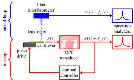
Figure 1: Schematic diagram of the experimental setup. In the red loop, the motion of the cantilever is transduced by a quantum point contact and amplified by an optimal controller, before being sent to a piezoelectric element mechanically coupled to the cantilever. The motion is also independently detected by an out-of-loop fiber interferometer, shown in blue.

The experimental setup described in this work is shown schematically in Fig. 1: the QPC transducer generates an electrical signal proportional to the cantilever displacement; such a signal is then amplified by a digital optimal controller Optcontrol and sent to a piezoelectric element mechanically coupled to the cantilever. We choose the phase of the optimal control feedback such that the cantilever oscillation is damped. Here we demonstrate the possibility to damp the thermal noise spectrum of the resonator below the QPC measurement noise floor, which is close to the shot noise level. Such an effect has already been demonstrated for an opto-electronic loop Buchler:1999 ; Bushev:2006 ; Poggio:2007 ; Lee:2010 and is known as intensity noise “squashing”. In such a regime, the effect on the motion of the resonator can be further validated by detecting it outside the feedback loop, by a second transducer whose measurement noise is not correlated with the motion. In this work, such an out-of-loop measurement has been carried out by means of a low-power laser interferometer.

The QPC transducer is made from a heterostructure grown by molecular-beam epitaxy on a (001) GaAs substrate; the structure consists of a 600 nm GaAs layer grown on top of the substrate, followed by 20 nm Al_0.25Ga_0.75As, a Si delta-doped layer, 40 nm Al_0.25Ga_0.75As and finally a 5 nm GaAs cap. The 2DEG lies only 65 nm below the surface and is characterized by a carrier density $n=2.5\times 10^{11}\,\mbox{cm}^{-2}$ and mobility $\mu=10^{5}\,\mbox{cm}^{2}\mbox{V}^{-1}\mbox{s}^{-1}$ at $T=4.2$ K. Ti/Au (5/15 nm) split gates patterned by electron-beam lithography define the QPC within the 2DEG. The application of a negative potential $V_{g}$ between the gates and the 2DEG forms a variable-width channel through which electrons flow. Ni/Ge/Au/Ni (2/26/54/15 nm) ohmic contacts are defined on either side of the channel, across which an applied source-drain voltage $V_{sd}$ drives the QPC conductance.

The micromechanical resonator is a commercial cantilever (Arrow TL1 from NanoWorld AG) made from monolithic silicon which is highly doped to make it conductive. The cantilever consists of a $(500\times 100\times 1)\,\mu$m shaft ending with a triangular sharp tip (radius of curvature around 10 nm) which has been metallized with Ti/Au (10/30 nm) to reduce the non-contact friction produced by the interaction with the QPC sample surface Stipe:2001 . Due to the cantilever conductivity, a voltage $V_{l}$ can be applied to its tip by contacting the base of the cantilever chip. At $T=4.2$ K, the cantilever has a resonant frequency $\nu_{0}=7.9$ kHz and an intrinsic quality factor $Q_{0}=2.0\times 10^{5}$, measured using a “ring-down” technique, by exciting the cantilever and measuring the decay of its oscillation amplitude. The oscillator spring constant is determined to be $k=2\times 10^{-3}$ N/m through measurements of its thermal noise spectrum at several different temperatures.

The cantilever and QPC are mounted in a vacuum chamber with a pressure below $10^{-6}$ torr at the bottom of a ⁴He cryostat ($T=4.2$ K), which is isolated from environmental vibrations. A two-tesla magnetic field, perpendicular to the QPC surface, is applied in order to reduce the backscattering of electrons in the conductance channel, thus providing a steeper conductance quantization; the field also has the effect of further damping the external vibrations of the system. A three-dimensional positioning stage with nanometer precision and stability (Attocube AG) moves the QPC relative to the cantilever.

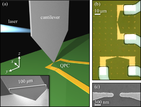
Figure 2: (a) Schematic picture of the experimental setup. The inset is a scanning electron micrograph of the cantilever tip, mounted on a silicon nitride blade to damp its vibrations. (b) Optical micrograph of the device containing two QPCs in different orientations with respect to the oscillation direction of the cantilever. (c) Scanning electron micrograph of the active region of the QPC.

The displacement measurement is made by positioning the tip of the cantilever about 80 nm above the QPC, as shown schematically in Fig. 2a. Owing to the proximity of the cantilever to the QPC itself, the cantilever’s tip and the QPC are capacitively coupled. The tip acts as a movable third gate above the device surface, able to affect the potential landscape of the QPC channel and thereby to alter its conductance $G$. A voltage $V_{g}$ applied to the two gates patterned on the surface modifies $G$ in the same manner.

The tip-QPC capacitive coupling strongly depends on their relative separation. Furthermore, the sensitivity of $G$ to the cantilever motion also depends on the relative orientation between the direction along which the cantilever oscillates and the one followed by the current flow. For studying this behavior, different QPCs have been defined on the same chip (Fig. 2b), with the split gates patterned such that a current flows either along the cantilever’s oscillation direction, or perpendicular to it; we have found the former to be the best orientation. In order to map the effect on the conductance by the position of the cantilever above the QPC device, $G$ has been recorded while scanning the cantilever at fixed distance $z$, with a potential $V_{l}$ applied. In such a conductance map, the position corresponding to the highest sensitivity is where the absolute value of the spatial derivative along the oscillation direction is maximum, as shown in Fig. 3.

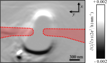
Figure 3: $\partial G/\partial x$ plotted as a function of the cantilever position over the QPC device, at a fixed distance $z=80$ nm. The red shaded areas show the position of the QPC gates. $V_{g}=-0.837$ V, $V_{l}=-1.280$ V. Data were processed with the WSxM software Horcas:2007 .

With the tip of the cantilever so positioned, the QPC acts as a transducer of the cantilever thermal motion. Its displacement resolution, without any feedback force, is shown in Fig. 4a, along with that of the low-power laser interferometer used in the out-of-loop measurement, shown in Fig. 4b. The resonances represent the cantilever fundamental mode and match in both frequency and quality factor. A DC source-drain voltage $V_{sd}=5.0$ mV drives a current through the QPC with voltages $V_{g}=-0.837$ V applied to the gates and $V_{l}=-1.280$ V to the cantilever. This configuration defines a conductance corresponding to one half the value of the first conductance quantum $2e^{2}/h$, where $e$ and $h$ are the electron charge and Plank’s constant respectively. Under the same conditions, we also measure the cantilever displacement using an optical fiber interferometer. The interferometer consists of 20 nW of laser light from a temperature-tuned 1,550-nm distributed feedback laser diode focused onto a region close to the cantilever tip and then reflected back onto the cleaved end of an optical fiber Bruland:1999 . The fiber end is coated with 25 nm of Si for optimal reflectivity. In order to express the QPC current response (left axis in Fig. 4a) in terms of cantilever motion (right axis), we have normalized the peak QPC current spectral density to the peak of the displacement response measured by the interferometer, obtaining a conductance response up to $0.002\,(2e^{2}/h)\,\mbox{nm}^{-1}$ of cantilever motion.

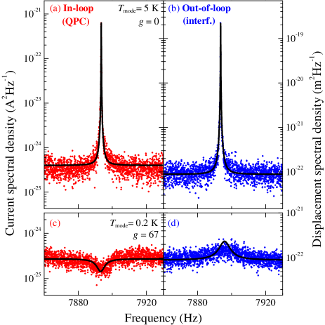
Figure 4: Cantilever fundamental mode spectrum detected at a base temperature $T=4.2$ K by (a, c) a QPC transducer, (b, d) a fiber interferometer. The QPC response is expressed in terms of both A² Hz^-1 (left axis) and m² Hz^-1 (right axis). (a) and (b) represent the cantilever thermal noise, (c) and (d) are the results of the application to the cantilever of a damping feedback force. In the measurements shown here, the QPC gives a conductance response of $2\times 10^{-4}\,(2e^{2}/h)\,\mbox{nm}^{-1}$ of cantilever motion.

For frequencies in the vicinity of the fundamental resonance mode, the motion of a cantilever is well approximated by the equation of a damped harmonic oscillator, driven by thermal force and, in case of a closed-loop system, also by a feedback force. In this work, we approximate the optimal control operated in the feedback loop as a force proportional to the displacement with a $\pi/2$ phase lag. In the experiment, the phase of the feedback signal is affected by the delay introduced by stray capacitances in the loop and it has been tuned in order to achieve the desired value $\pi/2$ for optimal damping Poot:2012 . The equation of motion of the cantilever can thus be written as:

$$m\ddot{x}+\Gamma_{0}\dot{x}+kx=F_{\text{th}}-g\Gamma_{0}\omega_{0}\,\delta(t-\pi/(2\omega_{0}))\otimes(x+x_{n}),$$ (1)

where $x(t)$ is the displacement of the oscillator as a function of time, $m$ is the oscillator effective mass, $\omega_{0}$ is its angular resonance frequency, $\Gamma_{0}=m\omega_{0}/Q_{0}$ is its intrinsic dissipation, $k=m\omega_{0}^{2}$ is its spring constant, $F_{\text{th}}$ is the random thermal Langevin force, $g$ is the feedback gain coefficient, $x_{n}(t)$ is the measurement noise on the displacement signal, $\delta$ is the Dirac distribution, and the symbol $\otimes$ denotes convolution.

Considering in (1) frequency components of the form $\hat{F}_{\text{th}}(\omega)\,e^{i\omega t}$ and $\hat{x}_{n}(\omega)\,e^{i\omega t}$, it is possible to determine the resonator displacement spectral density as measured in-loop ($S_{x}^{\text{il}}$) or out-of-loop ($S_{x}^{\text{ol}}$). To do so, we have followed the procedure described in Refs. Poggio:2007 ; Poot:2012 : the former involves the calculation of the white spectral density of the thermal force $F_{\text{th}}$ through the application of the fluctuation-dissipation theorem. The out-of-loop response is simply the sum of the actual displacement of the cantilever $S_{x}$ and the white spectral density of the interferometer measurement noise $S_{\xi_{n}}$. On the other hand, in the case of the in-loop response, feedback produces anticorrelations between the transduction noise and the mechanical motion of the cantilever. The resulting equations are:

$$S_{x}^{\text{il}} = \frac{\frac{4\omega_{0}^{3}k_{B}T}{Q_{0}k}+\left[\left(\omega_{0}^{2}-\omega^{2}\right)^{2}+\left(\frac{\omega_{0}\omega}{Q_{0}}\right)^{2}\right]S_{x_{n}}}{\left(\omega_{0}^{2}-\omega^{2}\right)^{2}+\left[\frac{\omega_{0}}{Q_{0}}\left(\omega+g\omega_{0}\right)\right]^{2}},$$ (2)

$$S_{x}^{\text{ol}} = S_{x}+S_{\xi_{n}}=\frac{\frac{4\omega_{0}^{3}k_{B}T}{Q_{0}k}+\left(\frac{g\omega_{0}^{2}}{Q_{0}}\right)^{2}S_{x_{n}}}{\left(\omega_{0}^{2}-\omega^{2}\right)^{2}+\left[\frac{\omega_{0}}{Q_{0}}\left(\omega+g\omega_{0}\right)\right]^{2}}+S_{\xi_{n}},$$ (3)

where $S_{x_{n}}$ is the white spectral density of the QPC measurement noise $x_{n}$, $k_{B}$ the Boltzmann constant and $T$ the bath temperature.

We fit the undamped in-loop and out-of-loop spectra in Figs. 4a, b with feedback gain $g=0$. We first fit the out-of-loop spectrum using (3) with three free parameters: $\omega_{0}$, $Q_{0}$ and $S_{\xi_{n}}$. Setting these parameters as constants, we then fit the in-loop spectrum with $S_{x_{n}}$ as the only free parameter. Both spectra are well-described by the fit functions. The value of $Q_{0}$ extracted from this procedure is equal to $8.0\times 10^{4}$ and is lower than that measured with the cantilever far from the QPC surface, due to unavoidable non-contact friction. $S_{x_{n}}$ and $S_{\xi_{n}}$ express the level of the noise floors for the in-loop and the out-of-loop measurements, respectively. They set the resolution of the QPC and the laser interferometer as displacement transducers, which is roughly the same for both: below $10^{-11}\,\mbox{m}/\sqrt{\mbox{Hz}}$.

The effective temperature of the fundamental mode does not depend on the measurement noise and is defined, according to the equipartition theorem, as:

$$T_{\text{mode}}=\frac{k}{2\pi k_{B}}\,\int^{\infty}_{0}S_{x}\,d\omega.$$ (4)

For the data in Figs. 4a and b, the value of $T_{\text{mode}}$ resulting from the equation above, using the expression of $S_{x}$ obtained from the fit, is equal to 5 K, which corresponds to the bath temperature $T$ of liquid helium.

We now describe the feedback cooling of the cantilever fundamental mode using the QPC transducer. Optimal control of the resonator motion in the feedback loop allows the damping of its fundamental mode oscillations and therefore the reduction of $T_{\text{mode}}$. Such an effect can be described with the application of a non-zero gain $g$ in the equation of motion (1). Increasing the value of $g$ produces anticorrelations between the in-loop transduction noise and the mechanical oscillator motion Bushev:2006 ; Poggio:2007 ; Lee:2010 . As a consequence, the displacement spectral density detected inside the feedback loop can even exhibit a dip below its noise floor near the oscillator’s resonant frequency, as shown in Fig. 4c. This spectrum represents noise “squashing” for a transduction scheme limited by electron, rather than photon, shot-noise. The solid line plotted along with this in-loop spectrum in Fig. 4c represents a fit computed using (2), with the value of $Q_{0}$ extracted previously and with $g$ as the free parameter.

In order to provide a validation of the observed phenomenon and an independent measurement of $T_{\text{mode}}$, the cantilever motion is also detected through the out-of-loop laser interferometer. This spectrum, shown in Fig. 4d, exhibits a peak above the uncorrelated measurement noise $S_{\xi_{n}}$. In order to compare our model with the measured data, we plot (3) as a solid line in Fig. 4d, using $Q_{0}$, $S_{x_{n}}$, and $S_{\xi_{n}}$ extracted from previous fits and $g$ extracted from the fit to the damped in-loop QPC spectrum of Fig. 4c. The plot of the out-of-loop spectrum highlights the agreement between our theoretical model and the experimental data.

To calculate the mode temperature, a general expression can be elaborated from (4), using the expression given in (3) for $S_{x}$; we find for $T_{\text{mode}}$ the same result obtained in Ref. Poggio:2007 , valid for a high quality factor:

$$T_{\text{mode}}=\frac{T}{1+g}+\frac{k\omega_{0}}{4k_{B}Q_{0}}\left(\frac{g^{2}}{1+g}\right)S_{x_{n}}.$$ (5)

The values of $T_{\text{mode}}$ resulting either from direct integration of the spectrum as in (4), or by extracting the parameters from the fit and then substituting them into (5), are equal within our precision: 0.2 K, twenty times less than the bath temperature.

Equation (5) implies that, in the limit $g\gg 1$, the minimum achievable temperature is:

$$T_{\text{mode}}^{\text{min}}=\sqrt{\frac{m\omega_{0}^{3}T}{k_{B}Q_{0}}S_{x_{n}}},$$ (6)

which in our case results to be $(0.21\pm 0.05)$ K, equal whithin the error to the observed value of $T_{\text{mode}}$ in the noise squashing regime.

In order to achieve the lowest possible mode temperature, thus accessing a state with a low occupation number ($N_{\text{mode}}=k_{B}T_{\text{mode}}/\hbar\omega_{0}$), future experiments should employ cantilevers with a low mass, low resonance frequency, and a high quality factor. The base temperature should also be lowered, by means of a ³He or a dilution refrigerator. In addition, lowering the measurement noise floor $S_{x_{n}}$ would represent a crucial improvement, involving both a decrease in the QPC current noise and an increase in the sensitivity of the QPC to the cantilever displacement. In the experiment presented here, the QPC noise floor is within a factor 10 above its current shot-noise limit; an improvement of the measurement setup would allow us to approach this limit. On the other hand, a better sensitivity could be achieved in two ways: improving the performance of the QPC as a one-dimensional conductor, and increasing the cantilever-QPC capacitive coupling. The former implies using a QPC defined on a 2DEG with a higher electron mobility and at a lower bath temperature. The effect would be to obtain a sharper QPC conductance quantization, and therefore a higher sensitivity to local electrostatic fields. The latter requires bringing the conductance channel closer to the cantilever tip, by using a QPC defined on a shallower 2DEG, optimizing the shape of the tip for a higher influence on the QPC potential landscape, and reducing shielding effects from both charged defects and gates on the QPC surface.

We acknowledge support from the Canton Aargau, the Swiss NSF (grant 200020 140478), the NCCR QSIT, and the US NSF.

References

- (1) D. Rugar, R. Budakian, H. J. Mamin, and B. W. Chui, Nature 430, 329 (2004).
- (2) J. Chaste, A. Eichler, J. Moser, G. Ceballos, R. Rurali, and A. Bachtold, Nature Nanotech. 7, 301 (2012).
- (3) S. E. Whitcomb, Class. Quantum Grav. 25, 114013 (2008).
- (4) S. Bose, K. Jacobs, and P. L. Knight, Phys. Rev. A 59, 3204 (1999).
- (5) M. Poot, H. S. J. van der Zant, Phys. Rep. 511, 273 (2012).
- (6) C. M. Caves, K. S. Thorne, R. W. P. Drever, V. D. Sandberg, M. Zimmermann, Rev. Modern Phys. 52, 341 (1980).
- (7) A. D. O’Connell et al., Nature 464, 697 (2010).
- (8) J. D. Teufel et al., Nature 475, 359 (2011).
- (9) J. Chan et al., Nature 478, 89 (2011).
- (10) I. Kozinsky, H. W. Ch. Postma, I. Bargatin, and M. L. Roukes, Appl. Phys. Lett. 88, 253101 (2006).
- (11) M. Poggio, C. L. Degen, H. J. Mamin, and D. Rugar, Phys. Rev. Lett. 99, 017201 (2007).
- (12) M. Poggio, M. P. Jura, C. L. Degen, M. A. Topinka, H. J. Mamin, D. Goldhaber-Gordon, and D. Rugar, Nature Phys. 4, 635 (2008).
- (13) A. A. Clerk, S. M. Girvin, and A. D. Stone, Phys. Rev. B 67, 165324 (2003).
- (14) A. A. Clerk, Phys. Rev. B 70, 245306 (2004).
- (15) J. L. Garbini, K. J. Bruland, W. M. Dougherty, and J. A. Sidles, J. Appl. Phys. 80, 1951 (1996); K. J. Bruland, J. L. Garbini, W. M. Dougherty, and J. A. Sidles, J. Appl. Phys. 80, 1959 (1996).
- (16) B. C. Buchler, M. B. Gray, D.A. Shaddock, T. C. Ralph, and D. E. McClelland, Opt. Lett. 24, 259 (1999).
- (17) P. Bushev, D. Rotter, A. Wilson, F. Dubin, C. Becher, J. Eschner, R. Blatt, V. Steixner, P. Rabl, and P. Zoller, Phys. Rev. Lett. 96, 043003 (2006).
- (18) K. H. Lee, T. G. McRae, G. I. Harris, J. Knittel, and W. P. Bowen, Phys. Rev. Lett. 104, 123604 (2010).
- (19) B. C. Stipe, H. J. Mamin, T. D. Stowe, T. W. Kenny, and D. Rugar, Phys. Rev. Lett. 87, 096801 (2001).
- (20) K. J. Bruland, J. L. Garbini, W. M. Dougherty, S. H. Chao, S. E. Jensen, and J. A. Sidles, Rev. Sci. Instrum. 70, 3542 (1999).
- (21) I. Horcas, R. Fernandez, J. M. Gomez-Rodriguez, J. Colchero, J. Gomez-Herrero, and A. M. Baro, Rev. Sci. Instrum. 78, 013705 (2007).