Self-force via energy-momentum
and angular momentum balance equations

Abstract

The radiation reaction for a point-like charge coupled to a massive scalar field is considered. The retarded Green’s function associated with the Klein-Gordon wave equation has support not only on the future light cone of the emission point (direct part), but extends inside the light cone as well (tail part). Dirac’s scheme of decomposition of the retarded electromagnetic field into the “mean of the advanced and retarded field” and the “radiation” field is adapted to theories where Green’s function consists of the direct and the tail parts. The Harish-Chandra equation of motion of radiating scalar charge under the influence of an external force is obtained. This equation includes effect of particle’s own field. The self force produces a time-changing inertial mass.

1 Introduction

There is an extensive literature devoted to the regularization problem in curved spacetime. De Witt and Brehme [1] derived the self-force acting upon a point electric charge in fixed background gravitational field. (Their expression for radiation reaction was later corrected by Hobbs [2].) The principle of equivalence in general relativity implies that a particle of infinitesimal mass and size moves along a geodesic. The particle of a small but finite mass perturbs the spacetime geometry. Mino, Sasaki and Tanaka [3] included the interaction of the particle with this perturbation which changes the worldline. In [4] Quinn has obtained an expression for the self-force on a point-like particle coupled to a massless scalar field. There is a long series of papers devoted to the motion of a point electric charge, a point scalar charge, and a point mass in black hole spacetimes, where the effects of radiation reaction are taken into account (see references in review [5]).

The computation of effect of particle’s own field is not a trivial matter, since the Green’s function associated with the wave operator has support within the light cone. This is because in curved spacetime massless waves propagate not just at a speed of light, but also at all speeds smaller than or equal to the speed of light. The particle may “fill” its own field, which acts on it just like an external one. The equation of motion require one to identify that portion of the retarded field at each point of the world line which arises from source contributions interior to the light cone. This part of field is often called the “tail term”. The self force on a particle then consists of two parts: this comes from the direct part of the Green’s function and depends on the current state of particle’s motion and that comes from the tail part and depends not only the current state of the particle, but also on its past history. It leads to the non-local (integro-differential) equations of motion.

Detweiler and Whiting proposed [6] a consistent decomposition of the retarded Green’s function into singular and radiative parts. It obeys the spirit of Dirac’s scheme of splitting of electromagnetic potential of a point-like charged particle arbitrarily moving in flat spacetime. Dirac [7] decomposed the retarded Liénard-Wiechert potential $A^{\rm ret}$ into two parts: (i) one-half of the retarded plus one-half of the advanced potentials which is inhomogeneous solution of the wave equation $\square A_{\alpha}=-4\pi j_{\alpha}$ whose source term is infinite on the world line. $A^{S}=1/2(A^{\rm ret}+A^{\rm adv})$ is just singular as the retarded potential in the immediate vicinity of the particle’s world line. The superscript “S” stands for “singular” as well as “symmetric”. (ii) combination $A^{R}=1/2(A^{\rm ret}-A^{\rm adv})$ of one-half of the retarded minus one-half of the advanced potentials which satisfies the homogeneous wave equation. This well behaved potential can be thought as a free radiation field. The superscript “R” stands for “radiative” as well as “regular”.

The radiative Green’s function implicitly used by Dirac in flat spacetime is

$$G^{\rm rad}(x,y)=G^{\rm ret}(x,y)-G^{\rm sym}(x,y)$$ (1.1)

where

$$G^{\rm sym}(x,y)=\frac{1}{2}\left[G^{\rm ret}(x,y)+G^{\rm adv}(x,y)\right].$$ (1.2)

The causal structure of the Green’s function is richer in curved spacetime. Due to contributions of the interior of the light cones, the retarded potential depends on the particle’s history prior to the retarded instant $\tau^{\rm ret}(x)$ while the advanced one is generated by portion of particle’s world line $\zeta$ after the advanced instant $\tau^{\rm adv}(x)$. (The retarded and the advanced moments label the points on $\zeta$ related with arbitrary field point $x\in{\mathbb{M}}_{\,4}$ by null rays.) The combination of half-retarded potential minus half-advanced one could satisfy the homogeneous wave equation. Moreover, it would be smooth on the world line. But a self-force constructed from this radiative potential will be highly non-causal. It will be depend on particle’s entire history, both past (through the retarded Green’s function) and future (through the advanced Green’s function). The Dirac’s scheme (1.1) for decomposition cannot be adopted without modification in curved spacetime. The modification is performed in Ref.[6].

Detweiler and Whiting start with a Hadamard construction of a symmetric scalar field Green’s function

$$G^{\rm sym}(x,y)=\frac{1}{8\pi}\left[u(x,y)\delta(\sigma)-v(x,y)\theta(-\sigma)\right],$$ (1.3)

where $u(x,y)$ and $v(x,y)$ are smooth functions of the base point $y$ and the field point $x$ and $\sigma$ is half of the square of the distance measured along the geodesic from $x$ to $y$. The step function $\theta(-\sigma)$ means that this part of $G^{\rm sym}(x,y)$ has support within both the past null cone and the future null cone of $x$. Having coupled it with $\delta-$shaped distribution of scalar charge moving along a geodesic we obtain the tail part of the field $\psi$ as follows:

$$\psi_{\rm tail}^{\rm sym}(x)=-\frac{q}{2}\left[\int_{-\infty}^{\tau^{\rm ret}(x)}{\rm d}\tau v(x,z(\tau))+\int^{+\infty}_{\tau^{\rm adv}(x)}{\rm d}\tau v(x,z(\tau))\right].$$ (1.4)

To remove the noncausality, authors add to singular Green’s function (1.3) biscalar $v(x,y)$ being solution of homogeneous wave equation. A new symmetric (singular) Green’s function

$$G^{\rm S}(x,y)=\frac{1}{8\pi}\left[u(x,y)\delta(\sigma)-v(x,y)\theta(\sigma)\right],$$ (1.5)

has no support within the null cone. Corresponding tail part of the scalar field depends on particle’s history during the interval $[\tau^{\rm ret}(x),\tau^{\rm adv}(x)]$:

$$\psi_{\rm tail}^{\rm S}(x)=\frac{q}{2}\left[\int_{\tau^{\rm ret}(x)}^{\tau^{\rm adv}(x)}{\rm d}\tau v(x,z(\tau))\right].$$ (1.6)

It is inhomogeneous solution of wave equation. Since it is singular just as the retarded tail field $\psi_{\rm tail}^{\rm ret}$(x), the authors define the radiative Green’s function as follows

$$G^{\rm R}(x,y)=G^{\rm ret}(x,y)-G^{\rm S}(x,y)$$ (1.7)

(cf. eq.(1.1)). Corresponding radiation field

$$\psi^{\rm R}(x)=-\left[\frac{qu(x,z(\tau))}{2\dot{\sigma}}\right]_{\tau^{\rm ret}(x)}^{\tau^{\rm adv}(x)}-q\left[\int_{-\infty}^{\tau^{\rm ret}(x)}{\rm d}\tau v(x,z(\tau))+\frac{1}{2}\int_{\tau^{\rm ret}(x)}^{\tau^{\rm adv}(x)}{\rm d}\tau v(x,z(\tau))\right]$$ (1.8)

is well behaved solution of homogeneous wave equation. In the coincidence limit, where field point $x$ approaches to the world line at point $z(\tau)$, the interval $[\tau^{\rm ret}(x),\tau^{\rm adv}(x)]$ shrinks to zero. Due to taking of this limit the potential (1.8) is generated by the portion of the world line that corresponds to the causal interval $]-\infty,\tau]$. The last integral in eq. (1.8) gives no contribution to a self-force because it cancels the ill defined part of gradient $\triangle_{\alpha}\psi_{\rm tail}^{\rm ret}$ coming from implicit dependence of $\tau^{\rm ret}$ upon $x$.

Following this scheme, Detweiler and Whiting recovered the results [1, 3, 4] for electromagnetic, scalar, and gravitational fields.

It is obvious that the physically relevant solution of the wave equation is the retarded potential. Teitelboim [8] derived the electromagnetic self-force in flat spacetime within the framework of retarded causality. The author substituted the retarded Liénard-Wiechert field in the Maxwell energy-momentum tensor density and calculated the flow of energy-momentum which flows across a space-like surface. Minkowski space was parameterized by four curvilinear coordinates. The first, proper time, labels points of emission placed on $\zeta$, the second one determines the surface (e.g., a tilted hyperplane which is orthogonal to particle’s 4-velocity at fixed instant of observation). Having integrated the stress-energy tensor over two angular variables that distinguish points on the surface, Teitelboim found the flow of energy-momentum mentioned above. The resulted expression depends on the particle’s individual characteristics (on its mass, its charge, its velocity and acceleration). In fact, the surface integration is equivalent to taking of coincidence limit in Dirac’s scheme. Abraham-Lorentz-Dirac expression for electromagnetic self-force is obtained in [8] via consideration of energy-momentum conservation.

Teitelboim [8] demonstrates that each of two terms which constitute Abraham radiation-reaction four-vector originates from the specific part of Maxwell energy-momentum tensor density. The author decomposes the stress-energy tensor into two divergent-free components: $\hat{T}={\hat{T}}_{\rm bnd}+{\hat{T}}_{\rm rad}$. Surface integration of the bound part ${\hat{T}}_{\rm bnd}$ results the flow which never gets far from the point-like source. It is permanently “attached” to the charge and is carried along with it. A charged particle cannot be separated from its bound electromagnetic “cloud” which has its own 4-momentum and angular momentum. “Bare” charge and electromagnetic “cloud” constitute new entity: dressed charged particle. ${\hat{T}}_{\rm bnd}$ contributes into particle’s inertia: 4-momentum of dressed charge $e$ contains, apart from usual velocity term, the extra term whose time derivative is exactly the negative of the Schott term:

$$p^{\mu}=mu^{\mu}-\frac{2e^{2}}{3}a^{\mu}.$$ (1.9)

Calculation of flux of the radiative component ${\hat{T}}_{\rm rad}$ yields the Larmor relativistic rate of radiated energy-momentum. This part of energy-momentum detaches itself from the charge and leads an independent existence.

In this paper we tend Teitelboim’s approach to allow contributions from interior of the light cone. For the clearest demonstration of the impact of our analysis, we refer to a point-like particle of mass $m$ and charge $e$ coupled to electromagnetic field in flat spacetime of three dimensions [9, 10]. In $2+1$ electrodynamics the retarded Green’s function associated with D’Alembert operator $\square=\eta^{\alpha\beta}\partial_{\alpha}\partial_{\beta}$ is supported within the light cone [11, 12]:

$$G^{\rm ret}_{2+1}(x,y)=\frac{\theta(x^{0}-y^{0}-|{\mathbf{x}}-{\mathbf{y}}|)}{\sqrt{-2\sigma(x,y)}}.$$ (1.10)

$\theta(x^{0}-y^{0}-|{\mathbf{x}}-{\mathbf{y}}|)$ is the light cone step function defined to be one if $x^{0}-y^{0}\geq|{\mathbf{x}}-{\mathbf{y}}|$ and defined to be zero otherwise. Synge’s world function in flat space-time is numerically equal to half the squared distance between $x$ and $y$: [5]

$$\sigma(x,y)=\frac{1}{2}\eta_{\alpha\beta}(x^{\alpha}-y^{\alpha})(x^{\beta}-y^{\beta}).$$ (1.11)

The analysis of the simplest model with tails will give more deep understanding of Detweiler and Whiting scheme of decomposition.

The paper is organized as follows. In Section 2 and 3, we define the scalar potentials and scalar field strengths. In Section 4 we split the energy-momentum and angular momentum carried by massive scalar field into bound and radiative parts. Extracting of radiated portions of Noether quantities is not a trivial matter, since the massive field holds energy and momentum near the source. In Section 5, we derive equation of motion of radiating scalar pole via analysis of energy-momentum and angular momentum balance equations. It is of great importance that conservation laws yield the Harish-Chandra equation of motion [13]. In Section 6, we discuss the result and its implications.

2 Green’s function and potentials

The dynamics of a point-like charge coupled to massive scalar field is governed by the action [14, 5]

$$I_{\rm total}=I_{\rm part}+I_{\rm int}+I_{\rm field}.$$ (2.1)

Here

$$I_{\rm field}=-\frac{1}{8\pi}\int{\rm d}^{4}x\left(\eta^{\alpha\beta}\varphi_{\alpha}\varphi_{\beta}+k_{0}^{2}\varphi^{2}\right)$$ (2.2)

is an action functional for a massive scalar field $\varphi$ in flat spacetime with metric tensor $\eta^{\alpha\beta}={\rm diag}(-1,1,1,1)$. The mass parameter $k_{0}$ is a constant with the dimension of reciprocal length. Its physical sense will be discussed below. The integration is performed over all the spacetime. The particle action is

$$I_{\rm part}=-m_{0}\int{\rm d}\tau\sqrt{-{\dot{z}}^{2}}$$ (2.3)

where $m_{0}$ is the bare mass of the particle which moves on a world line $\zeta\in{\mathbb{M}}_{\,4}$ described by relations $z^{\alpha}(\tau)$ which give the particle’s coordinates as functions of proper time; ${\dot{z}}^{\alpha}(\tau)={\rm d}z^{\alpha}(\tau)/{\rm d}\tau$. Finally, the interaction term is given by

$$I_{\rm int}=g\int{\rm d}\tau\sqrt{-{\dot{z}}^{2}}\varphi(z)$$ (2.4)

where $g$ is scalar charge carried by a point-like particle.

Variation on field variable $\varphi$ of action (2.1) yields the Klein-Gordon wave equation

$$\left(\square-k_{0}^{2}\right)\varphi(x)=-4\pi\rho(x),$$ (2.5)

where $\square=\eta^{\alpha\beta}\partial_{\alpha}\partial_{\beta}$ is the D’Alembert operator. We consider a scalar field $\varphi(x)$ with a point particle source

$$\rho(x)=g\int_{-\infty}^{+\infty}{\rm d}\tau\delta^{4}(x-z(\tau)),$$ (2.6)

where $g$ is coupling constant and $\delta^{4}(x-z(\tau))$ is a four-dimensional Dirac’s distribution localized on the world line: charge’s density is zero everywhere, except at the particle’s position where it is infinite.

The relevant wave equation for the Green’s function $G(x,y)$ is

$$\left(\square-k_{0}^{2}\right)G(x-y)=-\delta^{4}(x-y).$$ (2.7)

Its solution is the symmetric Green’s function [5, 14]

$$G^{\rm sym}(x-y)=\frac{1}{4\pi}\left[\delta(\sigma)-\frac{k_{0}}{\sqrt{-2\sigma}}J_{1}(k_{0}\sqrt{-2\sigma})\theta(-\sigma)\right],$$ (2.8)

where $J_{1}$ is the first order Bessel’s function whose argument contains Synge’s world function (1.11).

Convoluting the retarded Green’s function

$$G^{\rm ret}(x-y) = \theta(x^{0}-y^{0})G^{\rm sym}(x-y)$$

$$= \frac{1}{4\pi}\left[\frac{\delta(T-R)}{R}-\theta(T-R)\frac{k_{0}J_{1}(k_{0}\sqrt{T^{2}-R^{2}})}{\sqrt{T^{2}-R^{2}}}\right],$$

where $T=x^{0}-y^{0}$ and $R=|{\mathbf{x}}-{\mathbf{y}}|$ with charge density (2.6), we construct the massive scalar field. The delta-function in eq.(2) results direct term which is generated by a single event in space-time: the intersection of the world line and $x$’s past light cone. The Heaviside stepfunction extends the support to the segment of $\zeta$ that corresponds to the interval $\tau\in]-\infty,\tau^{\rm ret}(x)]$. Summing up the direct term and the tail term, we construct the retarded potential produced by an arbitrarily moving point-like source coupled to massive scalar field [14, 13, 15]:

$$\varphi^{\rm ret}(x)=\frac{g}{r}-g\int\limits_{-\infty}^{\tau^{\rm ret}(x)}{\rm d}\tau\frac{k_{0}J_{1}[k_{0}\sqrt{-(K\cdot K)}]}{\sqrt{-(K\cdot K)}}.$$ (2.10)

The first term is referred to the retarded point $z^{\rm ret}$ associated with $x$; $r$ is the retarded distance between $z^{\rm ret}$ and $x$. $K=x-z(\tau)$ is four-vector pointing from $z(\tau)\in\zeta$ to a point $x$ where the potential $\varphi$ is observed (see Figure 1).

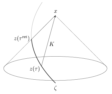
Figure 1: Direct part of the retarded potential at field point $x$ is generated by the intersection $z(\tau^{\rm ret})$ of the world line $\zeta$ and past light cone with vertex at $x$. Tail part of $\varphi^{\rm ret}(x)$ depends on the segment of $\zeta$ that corresponds to time interval $]-\infty,\tau^{\rm ret}(x)]$. The tail term defines contribution from cone’s interior. The vector $K$ is a vector pointing from the point of emission $z(\tau)\in\zeta$ to a field point $x$.

Convolution of the advanced Green’s function

$$G^{\rm adv}(x-y) = \theta(-x^{0}+y^{0})G^{\rm sym}(x-y)$$

$$= \frac{1}{4\pi}\left[\frac{\delta(T+R)}{R}-\theta(-T-R)\frac{k_{0}J_{1}(k_{0}\sqrt{T^{2}-R^{2}})}{\sqrt{T^{2}-R^{2}}}\right]$$

coupled with the $\delta$-like density (2.6) is analogous to the manipulations with its retarded counterpart. The advanced potential

$$\varphi^{\rm adv}(x)=\frac{g}{r_{\rm adv}}-g\int\limits^{+\infty}_{\tau^{\rm adv}(x)}{\rm d}\tau\frac{k_{0}J_{1}[k_{0}\sqrt{-(K\cdot K)}]}{\sqrt{-(K\cdot K)}}$$ (2.12)

is generated by the point charge during its entire future history following the advanced time associated with $x$ (see Figure 2). Particle’s characteristics in the direct term are referred to the instant $\tau^{\rm adv}(x)$.

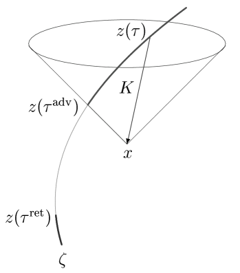
Figure 2: The advanced Green’s function (2) possesses support on the surface of the future light cone of $x$ (direct part) as well as within this cone (tail part). The portion of the world line after $\tau^{\rm adv}(x)$ produces the advanced potential (2.12). Advanced instant labels point at which particle’s world line punctures future light cone with vertex at $x$.

The simplest scalar field is generated by an unmoved source placed at the coordinate origin [17, 18]:

$$\varphi_{\rm Yu}(x)=g\frac{\exp(-k_{0}r)}{r}.$$ (2.13)

Here $r=\sqrt{(x^{1})^{2}+(x^{2})^{2}+(x^{3})^{2}}$ is the distance to the charge. It is the well-known Yukawa potential which plays an important role in the theory of nucleon-nucleon interactions.

3 Scalar field strengths

Let two particles interact through a massive scalar field. Static charge $g_{1}$ placed at the coordinate origin generates the Yukawa field with components

$$\Phi_{i}(x) = \frac{\partial\varphi_{\rm Yu}}{\partial x^{i}}$$

$$= -g_{1}\frac{e^{-k_{0}r}}{r^{2}}\left(1+k_{0}r\right)n_{i},$$

where $n_{i}=x_{i}/r$ is unit direction vector and $r$ is the distance to the charge. This charge exerts another one, say $g_{2}$, with the force

$${\mathbf{F}}_{12}=-g_{1}g_{2}\frac{e^{-k_{0}r_{12}}}{r_{12}^{2}}\left(1+k_{0}r\right){\mathbf{n}}_{12},$$ (3.2)

where ${\mathbf{n}}_{12}$ is unit vector codirectional with the radius vector ${\mathbf{r}}_{12}$ drawing from particle $1$ to particle $2$. The force is attractive if $g_{1}$ and $g_{2}$ are of like sign. The charges can be interpreted as nucleons which attract each other and are bound in a nucleus. The force (3.2) elucidates also why a neutron repels an antineutron.

In general, the action (2.1) can be considered as a classical version of the Yukawa model for strongly interacting nucleons. It is assumed that the neutrons and protons are joint together by a massive pseudoscalar pion field. Parameter $k_{0}$ associates with the rest mass of a massive scalar field particle mediating the interaction. The parameter acts as a cutoff: the heavier is the field particle, the shorter is range of Yukawa force. Yukawa force is essential at a distance about $1/k_{0}$.

Let us derive the field produced by an arbitrarily moving scalar charge. Scalar field strengths are given by the gradient of the potential (2.10). Differentiation of the direct term yields

$$\frac{\partial\varphi^{\rm ret}_{\rm dir}(x)}{\partial x^{\mu}}=-g\left[\frac{[1+(K\cdot a)]K_{\mu}}{r^{3}}-\frac{u_{\mu}}{r^{2}}\right]_{\tau=\tau^{\rm ret}(x)}.$$ (3.3)

Further we differentiate the tail term in the potential (2.10) which arises from source contributions interior to the light cone. Apart from the integral

$$\Phi_{\mu}^{(\theta)}(x)=g\int\limits_{-\infty}^{\tau^{\rm ret}(x)}{\rm d}\tau k_{0}^{2}\frac{{\rm d}}{{\rm d}W}\left(\frac{J_{1}(W)}{W}\right)k_{0}\frac{K_{\mu}}{\sqrt{-(K\cdot K)}}$$ (3.4)

the gradient $\Phi_{{\rm tail},\mu}=\Phi_{\mu}^{(\theta)}+\Phi_{\mu}^{(\delta)}$ contains also local term

$$\Phi_{\mu}^{(\delta)}(x)=gk_{0}^{2}\left.\frac{J_{1}(W)}{W}\frac{K_{\mu}}{r}\right|_{\tau=\tau^{\rm ret}}$$ (3.5)

which is due to time-dependent upper limit of integral in eq.(2.10). Argument of Bessel’s function $W:=k_{0}\sqrt{-(K\cdot K)}$.

To simplify the tail contribution us much us possible we use the identity

$$\frac{k_{0}}{\sqrt{-(K\cdot K)}}=\frac{1}{(K\cdot u)}\frac{{\rm d}W}{{\rm d}\tau}$$ (3.6)

in the integral (3.4) and perform integration by parts. On rearrangement, we add it to the expression (3.5). The term which depends on the end points only annuls $f_{\mu}^{(\delta)}$. Finally, the gradient of tail term of the potential (2.10) becomes

$$\frac{\partial\varphi^{\rm ret}_{\rm tail}(x)}{\partial x^{\mu}}=g\int\limits_{-\infty}^{\tau^{\rm ret}(x)}{\rm d}\tau k_{0}^{2}\frac{J_{1}(W)}{W}\left[\frac{1+(K\cdot a)}{r^{2}}K_{\mu}-\frac{u_{\mu}}{r}\right].$$ (3.7)

The particle’s position, velocity, and acceleration under the integral sign are evaluated at instant $\tau\leq\tau^{\rm ret}(x)$. The invariant quantity

$$r=-(K\cdot u)$$ (3.8)

is an affine parameter on the time-like geodesic that links $x$ to $z(\tau)$; it can be loosely interpreted as the time delay between $x$ and $z(\tau)$ as measured by an observer moving with the particle. (For such hypothetic observer the particle is momentarily at rest: its four-velocity $u^{\alpha}=(1,0,0,0)$.)

Because of asymptotic behavior of the first order Bessel’s function with argument $W:=k_{0}\sqrt{-(K\cdot K)}$ the retarded field

$$\Phi_{\mu}^{\rm ret}(x) = \frac{\partial\varphi^{\rm ret}(x)}{\partial x^{\mu}}$$

$$= -g\frac{1+(K\cdot a)}{r^{3}}K_{\mu}+g\frac{u_{\mu}}{r^{2}}+g\int\limits_{-\infty}^{\tau^{\rm ret}(x)}{\rm d}\tau k_{0}^{2}\frac{J_{1}(W)}{W}\left[\frac{1+(K\cdot a)}{r^{2}}K_{\mu}-\frac{u_{\mu}}{r}\right]$$

is finite on the light cone where $W=0$. It diverges on the particle’s trajectory only. Indeed, if the point of emission $z(\tau)$ approaches the field point $x$, all the components of four-vector $K=x-z(\tau)$ becomes infinitesimal ones and the distance (3.8) tends to zero.

The advanced field

$$\Phi_{\mu}^{\rm adv}(x) = \frac{\partial\varphi^{\rm adv}(x)}{\partial x^{\mu}}$$

$$= -g\frac{1+(K\cdot a)}{(r_{\rm adv})^{3}}K_{\mu}-g\frac{u_{\mu}}{(r_{\rm adv})^{2}}+g\int\limits^{+\infty}_{\tau^{\rm adv}(x)}{\rm d}\tau k_{0}^{2}\frac{J_{1}(W)}{W}\left[\frac{1+(K\cdot a)}{r^{2}}K_{\mu}-\frac{u_{\mu}}{r}\right]$$

depends on particle’s future history (see Figure 2). Particle’s characteristics in the direct part are referred to the advanced instant $\tau^{\rm adv}(x)$.

4 Scalar radiation

The action (2.1) is invariant under infinitesimal transformations (translations and rotations) which constitute the Poincaré group. According to Noether’s theorem, these symmetry properties yield conservation laws, i.e. those quantities that do not change with time. Outgoing radiation removes energy, momentum, and angular momentum from the source. The quantities are defined in standard way [19], as flows of the stress-energy tensor density $\hat{T}$

$$p_{\rm sc}^{\nu}(\tau)=\int_{\Sigma}{\rm d}\sigma_{\mu}T_{\rm sc}^{\mu\nu},$$ (4.1)

and its torque

$$M_{\rm sc}^{\mu\nu}(\tau)=\int_{\Sigma}{\rm d}\sigma_{\alpha}\left(x^{\mu}T_{\rm sc}^{\nu\alpha}-x^{\nu}T_{\rm sc}^{\mu\alpha}\right),$$ (4.2)

that flow across a space-like surface $\Sigma$ which intersects a world line at point $z(\tau)$; ${\rm d}\sigma_{\mu}$ is the vectorial surface element on $\Sigma$. While the stress-energy tensor is quite different than that in classical electrodynamics:

$$4\pi T_{\mu\nu}=\frac{\partial\varphi}{\partial x^{\mu}}\frac{\partial\varphi}{\partial x^{\nu}}-\frac{\eta_{\mu\nu}}{2}\left(\eta^{\alpha\beta}\frac{\partial\varphi}{\partial x^{\alpha}}\frac{\partial\varphi}{\partial x^{\beta}}+k_{0}^{2}\varphi^{2}\right),$$ (4.3)

(see Refs.[18, 20, 21]). To prepare the way for our discussion of a self-force acted on a point-like source coupled with massive scalar field, we consider first the relatively simple case of a massless scalar field.

4.1. Massless scalar radiation

Let parameter $k_{0}=0$. The rate of change of the energy-momentum of the retarded field is computed by means of the stress-energy tensor (4.3) where field tensor components are replaced by the direct field strengths (3.3). We call the part of massless scalar field which scales as $r^{-1}$ the radiative part of field:

$$\Phi_{\mu}^{\rm rad}(x)=-\frac{e}{r}(a\cdot k)k_{\mu}.$$ (4.4)

(Null vector $k^{\mu}=K^{\mu}/r$ is normalized in such a way that scalar product $(k\cdot u)=-1$.) The part which scales as $r^{-2}$ does not involve the acceleration:

$$\Phi_{\mu}^{\rm bnd}(x)=-\frac{e}{r^{2}}\left(k_{\mu}-u_{\mu}\right).$$ (4.5)

This is the bound part of field. Following Teitelboim [8], we decompose the stress-energy tensor into bound and radiative parts which are separately conserved off the world line. To calculate the radiative part it is straightforward to substitute eq.(4.4) into eq.(4.3):

$$4\pi T_{\rm rad}^{\mu\nu}=\frac{g^{2}}{r^{2}}(a\cdot k)^{2}k^{\mu}k^{\nu}.$$ (4.6)

The bound part

$$4\pi T_{\rm bnd}^{\mu\nu}=T_{(-4)}^{\mu\nu}+T_{(-3)}^{\mu\nu}$$ (4.7)

is the combinations of terms which depend on the retarded distance as $r^{-4}$ and $r^{-3}$, respectively:

$$4\pi T_{(-4)}^{\mu\nu} = \frac{g^{2}}{r^{4}}\left(k^{\mu}k^{\nu}-k^{\mu}u^{\nu}-u^{\mu}k^{\nu}+u^{\mu}u^{\nu}-\frac{1}{2}\eta^{\mu\nu}\right),$$ (4.8)

$$4\pi T_{(-3)}^{\mu\nu} = \frac{g^{2}}{r^{3}}(a\cdot k)\left(\phantom{\frac{1}{1}}\!\!\!\!2k^{\mu}k^{\nu}-k^{\mu}u^{\nu}-u^{\mu}k^{\nu}-\eta^{\mu\nu}\right).$$ (4.9)

To decompose the angular momentum tensor density

$$M^{\mu\nu\alpha}=x^{\mu}T^{\nu\alpha}-x^{\nu}T^{\mu\alpha}.$$ (4.10)

into the bound component and the radiative component, we use the formulae presented firstly in pioneer work [22]:

$$M_{\rm bnd}^{\mu\nu\alpha} = z^{\mu}T_{\rm bnd}^{\nu\alpha}-z^{\nu}T_{\rm bnd}^{\mu\alpha}+K^{\mu}T_{\rm(-4)}^{\nu\alpha}-K^{\nu}T_{\rm(-4)}^{\mu\alpha},$$ (4.11)

$$M_{\rm rad}^{\mu\nu\alpha} = x^{\mu}T_{\rm rad}^{\nu\alpha}-x^{\nu}T_{\rm rad}^{\mu\alpha}+K^{\mu}T_{\rm(-3)}^{\nu\alpha}-K^{\nu}T_{\rm(-3)}^{\mu\alpha}.$$ (4.12)

We enclose particle’s world line by a very thin tube [17] of constant radius $r$ and calculate fluxes of the stress-energy tensor (4.1) and its torque (4.2) through this surface. An appropriate coordinates are the retarded coordinates [5, Chapt.II] locally given by

$$x^{\alpha}=z^{\alpha}(s)+rk^{\alpha}.$$ (4.13)

Here $z(s)\in\zeta$ is the retarded point associated with a field point $x$, $r$ is the retarded distance between these points, and $k^{\alpha}(x)$ is a null vector field tangent to the congruence of null rays that emanate from $z(s)$.

Globally, the flat space-time ${\mathbb{M}}_{\,4}$ can be thought as a disjoint union of world tubes of all possible radii $r>0$. A world tube is a disjoint union of spheres of constant radii $r$ centered on a world line of the particle. The sphere $S(z(s),r)$ is the intersection of the future light cone generated by null rays emanating from point $z(s)\in\zeta$ in all possible directions

$$C^{+}(z(s))=\{x\in{\mathbb{M}}_{\,4}:\eta_{\alpha\beta}\left(x^{\alpha}-z^{\alpha}(s)\right)\left(x^{\beta}-z^{\beta}(s)\right)=0,x^{0}-z^{0}(s)>0\}$$ (4.14)

and the tilted hyperplane

$$\Sigma(z(s),r)=\{x\in{\mathbb{M}}_{\,4}:u_{\alpha}(s)\left(x^{\alpha}-z^{\alpha}(s)-u^{\alpha}(s)r\right)=0\}.$$ (4.15)

Points on the sphere $S(z(s),r)=C^{+}(z(s))\cap\Sigma(z(s),r)$ are distinguished by pair of angles: polar angle $\vartheta$ and azimuthal one $\varphi$, which specify direction of null vector $k$ (see. [5, Chapt.II, Fig.7]).

A point in Minkowski space can be specified therefore by means of curvilinear coordinates $(s,r,\vartheta,\varphi)$. To define a retarded coordinate system, we choose an origin point $z(s)$ on particle’s world line, future light cone (4.14) with vertex at this point, and tilted hyperplane (4.15) orthogonal to particle’s four-velocity $u(s)$. The relation between Minkowski coordinates and retarded coordinates is given by eq.(4.13).

We restrict ourselves to calculation of radiative parts of energy, momentum, and angular momentum. The technique developed in Ref.[23] can be easily adapted to this task. The outward directed surface element ${\rm d}\sigma_{\mu}$ of the cylinder $r=const$ is

$${\rm d}\sigma_{\mu}=r^{2}\left[-u_{\mu}+(1+ra_{k})k_{\mu}\right]{\rm d}s\wedge{\rm d}\Omega,$$ (4.16)

where $a_{k}:=(a\cdot k)$ is the component of particle’s acceleration in the direction $k$ and ${\rm d}\Omega=\sin\vartheta{\rm d}\vartheta\wedge{\rm d}\varphi$ is the element of a solid angle. The radiative part of energy-momentum carried by the massless scalar field is

$$p_{\rm dir,R}^{\nu}(\tau) = \int_{\Sigma_{r}}{\rm d}\sigma_{\mu}T_{\rm rad}^{\mu\nu}$$

$$= \frac{1}{4\pi}\int\limits_{-\infty}^{\tau}{\rm d}s\int{\rm d}\Omega r^{2}\left[-u_{\mu}+(1+ra_{k})k_{\mu}\right]\frac{g^{2}}{r^{2}}(a\cdot k)^{2}k^{\mu}k^{\nu}$$

$$= \frac{g^{2}}{3}\int\limits_{-\infty}^{\tau}{\rm d}sa^{2}(s)u^{\nu}(s).$$

Integration over angular variables is handled via the relations [23]:

$$\frac{1}{4\pi}\int{\rm d}\Omega=1,$$ (4.18)

$$\frac{1}{4\pi}\int{\rm d}\Omega k^{\alpha}=u^{\alpha},$$

$$\frac{1}{4\pi}\int{\rm d}\Omega k^{\alpha}k^{\beta}=\frac{4}{3}u^{\alpha}u^{\beta}+\frac{1}{3}\eta^{\alpha\beta},$$

$$\frac{1}{4\pi}\int{\rm d}\Omega k^{\alpha}k^{\beta}k^{\gamma}=2u^{\alpha}u^{\beta}u^{\gamma}+\frac{1}{3}u^{\alpha}\eta^{\beta\gamma}+\frac{1}{3}u^{\beta}\eta^{\alpha\gamma}+\frac{1}{3}u^{\gamma}\eta^{\alpha\beta}.$$

The computation of radiated angular momentum is virtually identical to that presented above and we do not bother with details. Resulting expression is as follows:

$$M_{\rm dir,R}^{\mu\nu}(\tau) = \frac{g^{2}}{3}\int_{-\infty}^{\tau}{\rm d}s\left\{\phantom{\frac{1}{1}}\!\!\!\!a^{2}(s)\left[\phantom{\frac{1}{1}}\!\!\!\!z^{\mu}(s)u^{\nu}(s)-z^{\nu}(s)u^{\mu}(s)\right]\right.$$

$$+ \left.u^{\mu}(s)a^{\nu}(s)-u^{\nu}(s)a^{\mu}(s)\phantom{\frac{1}{1}}\!\!\!\!\right\}.$$

We see that the radiated energy-momentum carried by massless scalar field is equal to one-half of the well-known Larmor rate of radiation integrated over the world line. Similarly, the radiated angular momentum is equal to the one-half of corresponding quantity in classical electrodynamics [22]. This finding is in line with expressions obtained in [13, 15, 16] for massless scalar self-force.

4.2. Radiation carried by massive scalar field

In this Section we decompose the energy-momentum and angular momentum carried by massive scalar field into the bound and radiative parts. The bound terms will be absorbed by particle’s individual characteristics while the radiative terms exert the radiation reaction. We do not calculate the flows of the massive scalar field across a thin tube around a world line of the source. To extract the appropriate finite parts of energy-momentum and angular momentum we apply the scheme developed in Refs.[9, 10]. The scheme summarizes cumbersome calculations of flows of energy, momentum, and angular momentum carried by electromagnetic field of a point-like source arbitrarily moving in flat space-time of three dimensions. In $2+1$ electrodynamics both the electromagnetic potential and the electromagnetic field are non-local: they depend not only on the current state of motion of the particle, but also on its past (or future) history. The scalar field strengths (3) and (3) behave analogously.

To find the tail parts of radiated Noether quantities sourced by the interior of light cone we deal with the retarded and the advanced fields defined on the world line only:

$$F_{\mu}^{\rm ret} = g\int_{-\infty}^{\tau_{1}}{\rm d}\tau_{2}f(z_{1},z_{2}),$$ (4.20)

$$F_{\mu}^{\rm adv} = g\int^{\tau}_{\tau_{1}}{\rm d}\tau_{2}f(z_{1},z_{2}).$$ (4.21)

The integrand is

$$f_{\mu}(z_{1},z_{2})=gk_{0}\frac{J_{1}[k_{0}\sqrt{-(q\cdot q)}]}{\sqrt{-(q\cdot q)}}\left[\frac{1+(q\cdot a_{2})}{r_{2}^{2}}q_{\mu}-\frac{u_{2,\mu}}{r_{2}}\right]$$ (4.22)

where $w=k_{0}\sqrt{-(q\cdot q)}$. Time-like vector $q^{\mu}=z_{1}^{\mu}-z_{2}^{\mu}$ connects an emission point $z(\tau_{2})\in\zeta$ with a field point $z(\tau_{1})\in\zeta$; $r_{2}=-(q\cdot u_{2})$. In the forthcoming expressions up to the end of the present paper index $1$ indicates that the particle’s velocity or position is referred to the instant $\tau_{1}\in]-\infty,\tau]$ while index $2$ says that the particle’s characteristics are evaluated at instant $\tau_{2}$ before $\tau$.

Let’s explain how these fields appeared. In case we do decide to integrate of energy and momentum densities over $\Sigma$ [9], we should study of interference of outgoing scalar waves emitted by different points on particle’s world line. This is because massive scalar waves propagate not just at a speed of light, but also at all speeds smaller than or equal to the speed of light. The world tube is not convenient to study the interference. The tilted hyperplane which plays privileged role in the radiation reaction problem in classical electrodynamics [8] is not suitable for our purpose too. The reason is that there is no a plane which is orthogonal to the particle’s 4-velocities at all points on $\zeta$ before the end point $z(\tau)=\zeta\cap\Sigma$. In Refs.[9, 10] we choose the simplest plane $\Sigma_{t}=\{x\in{\mathbb{M}}_{\,3}:x^{0}=t\}$ associated with an unmoving inertial observer. Non-covariant terms arise unavoidable due to integration over this surface. To reveal meaningful contribution in radiated energy-momentum we apply the criteria which were first formulated in [8, Table 1]:

• the bound term diverges while the radiative one is finite;

• the bound component depends on the momentary state of the particle’s motion while the radiative one is accumulated with time; and

• the form of the bound terms heavily depends on choosing of an integration surface while the radiative terms are invariant.

Since the stress-energy tensor, either electromagnetic or scalar, is quadratic in field strengths, we should twice integrate it over $\zeta$ in order to calculate its flux (4.1) through $\Sigma_{t}$. Figures 3 and 4 picture the interference of the disk emanated by fixed point $z(\tau_{1})\in\zeta$ with radiation generated by portion of the world line from the remote past to the observation instant $\tau$. Cumbersome calculations performed in [9] can be summarized as a simple scheme which can be easily adopted to case of massive scalar field.

      

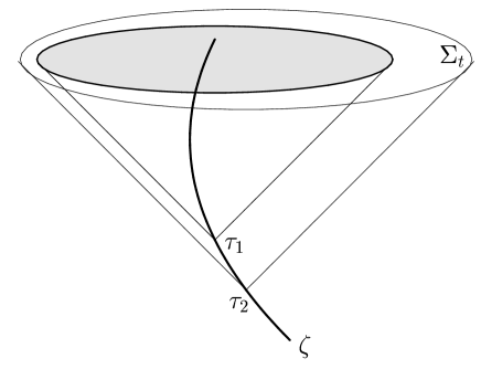
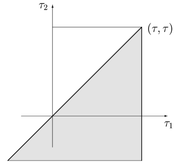
Figure 3: Outgoing scalar waves generated by the portion of the world line that corresponds to the interval $-\infty<\tau_{2}<\tau_{1}$ combine within the gray disk in the plane $\Sigma_{t}=\{x\in{\mathbb{M}}_{\,4}:x^{0}=t\}$. Corresponding domain of integration is $\int_{-\infty}^{\tau}{\rm d}\tau_{1}\int_{-\infty}^{\tau_{1}}{\rm d}\tau_{2}\int_{0}^{k_{1}^{0}}{\rm d}R\int{\rm d}\Omega$ where $k_{1}^{0}$ is the radius of smaller disk. After integration over spherical variables the domain reduces to double path integral $\int_{-\infty}^{\tau}{\rm d}\tau_{1}\int_{-\infty}^{\tau_{1}}{\rm d}\tau_{2}$. It is sketched on the right figure. It is obvious that this domain is equivalent to $\int_{-\infty}^{\tau}{\rm d}\tau_{2}\int^{\tau}_{\tau_{1}}{\rm d}\tau_{1}$.

      

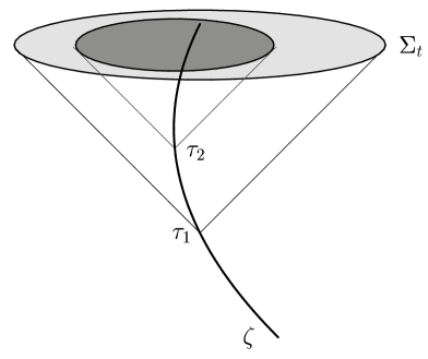
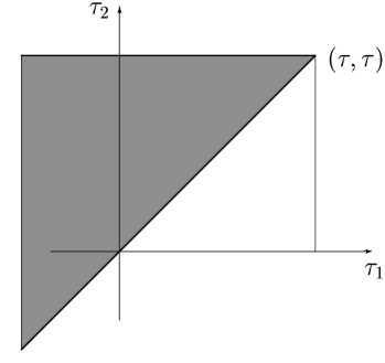
Figure 4: Outgoing scalar waves generated by the portion of the world line that corresponds to the interval $\tau_{1}<\tau_{2}\leq\tau$ joint together inside the dark disk. The domain of integration is $\int_{-\infty}^{\tau}{\rm d}\tau_{1}\int^{\tau}_{\tau_{1}}{\rm d}\tau_{2}\int_{0}^{k_{2}^{0}}{\rm d}R\int{\rm d}\Omega$ where $k_{2}^{0}$ is the radius of dark disk. After integration over spherical coordinates which parameterize $\Sigma_{t}$, the double integral $\int_{-\infty}^{\tau}{\rm d}\tau_{1}\int^{\tau}_{\tau_{1}}{\rm d}\tau_{2}$ survives. It can be replaced by $\int_{-\infty}^{\tau}{\rm d}\tau_{2}\int^{\tau_{2}}_{-\infty}{\rm d}\tau_{1}$.

1. Integration of the stress-energy tensor density over $\Sigma_{t}$ yields action at a distance theory which manipulates with fields evaluated on the world line only.

2. In case of combination of waves pictured in Fig.3 the surface integration (4.1) of the stress-energy tensor contributes in radiated energy-momentum one-half of the work

   $$p_{\rm ret}^{\mu}=-\frac{1}{2}\int_{-\infty}^{\tau}{\rm d}\tau_{1}F_{\rm ret}^{\mu}(\tau_{1})$$ (4.23)

   of the retarded tail force (4.20) acting on the charge itself. (The charge “fills” its own massive field just as an external one.)

   The surface integration of the angular momentum tensor density (4.2) gives one-half of the path integral of the torque of force (4.20):

   $$M_{\rm ret}^{\mu\nu}=-\frac{1}{2}\int_{-\infty}^{\tau}{\rm d}\tau_{1}\left[z_{1}^{\mu}F_{\rm ret}^{\nu}(\tau_{1})-z_{1}^{\nu}F_{\rm ret}^{\mu}(\tau_{1})\right].$$ (4.24)

3. Interference of outgoing scalar waves pictured in Fig.4 takes away from radiated energy-momentum one-half of the work

   $$p_{\rm adv}^{\mu}=-\frac{1}{2}\int_{-\infty}^{\tau}{\rm d}\tau_{1}F_{\rm adv}^{\mu}(\tau_{1})$$ (4.25)

   of the advanced tail force (4.21) acting on the charge itself. The surface integration of the angular momentum tensor density gives one-half of the path integral of the torque of advanced force (4.21):

   $$M_{\rm adv}^{\mu\nu}=-\frac{1}{2}\int_{-\infty}^{\tau}{\rm d}\tau_{1}\left[z_{1}^{\mu}F_{\rm adv}^{\nu}(\tau_{1})-z_{1}^{\nu}F_{\rm adv}^{\mu}(\tau_{1})\right].$$ (4.26)

4. The the support of double integral $\int_{-\infty}^{\tau}{\rm d}\tau_{1}\int_{\tau_{1}}^{\tau}{\rm d}\tau_{2}$ coincides with the support of the integral $\int_{-\infty}^{\tau}{\rm d}\tau_{2}\int_{-\infty}^{\tau_{2}}{\rm d}\tau_{1}$ (see Figs. 3 and 4). Since instants $\tau_{1}$ and $\tau_{2}$ label different points at the same world line $\zeta$, one can interchanges the indices “first” and “second” in the integrand. Via interchanging of these indices we finally obtain $\int_{-\infty}^{\tau}{\rm d}\tau_{1}\int_{-\infty}^{\tau_{1}}{\rm d}\tau_{2}g(\tau_{2},\tau_{1})$ instead of initial $\int_{-\infty}^{\tau}{\rm d}\tau_{1}\int_{\tau_{1}}^{\tau}{\rm d}\tau_{2}g(\tau_{1},\tau_{2})$.

5. The radiative part of energy-momentum carried by massive scalar field is therefore

   $$p^{R}_{{\rm tail},\mu} =- \frac{1}{2}\int_{-\infty}^{\tau}{\rm d}\tau_{1}\left(F^{\rm ret}_{\mu}-F^{\rm adv}_{\mu}\right)$$

   $$= -\frac{g^{2}}{2}\int_{-\infty}^{\tau}{\rm d}\tau_{1}\int_{-\infty}^{\tau_{1}}{\rm d}\tau_{2}\left(f_{\mu}(z_{1},z_{2})-f_{\mu}(z_{2},z_{1})\right).$$

   Both the radiated angular momentum

   $$M^{R}_{{\rm tail},\mu\nu} = -\frac{1}{2}\int_{-\infty}^{\tau}{\rm d}\tau_{1}\left[z_{1,\mu}\left(F^{\rm ret}_{\nu}-F^{\rm adv}_{\nu}\right)-z_{1,\nu}\left(F^{\rm ret}_{\mu}-F^{\rm adv}_{\mu}\right)\right]$$

   $$= -\frac{g^{2}}{2}\int_{-\infty}^{\tau}{\rm d}\tau_{1}\int_{-\infty}^{\tau_{1}}{\rm d}\tau_{2}\left\{\!\!\!\!\phantom{\frac{1}{1}}z_{1,\mu}f_{\nu}(z_{1},z_{2})-z_{1,\nu}f_{\mu}(z_{1},z_{2})\right.$$

   $$- \left.\left[z_{2,\mu}f_{\nu}(z_{2},z_{1})-z_{2,\nu}f_{\mu}(z_{2},z_{1})\right]\!\!\!\!\phantom{\frac{1}{1}}\right\}.$$

   and energy-momentum (5) exert the radiation reaction.

Now we evaluate the “upper-limit” behavior of the tail Noether quantities. By this we mean the coincidence limit $\tau_{2}\to\tau_{1}$ of the of the expressions under the double integrals in eqs. (5) and (5), namely

$$p_{\rm tail,R}^{\mu}=-\frac{g^{2}}{2}\int_{-\infty}^{\tau}{\rm d}\tau_{1}\int_{-\infty}^{\tau_{1}}{\rm d}\tau_{2}k_{0}^{2}\frac{J_{1}(w)}{w}\left[\frac{1+(q\cdot a_{2})}{r_{2}^{2}}q^{\mu}-\frac{u_{2}^{\mu}}{r_{2}}+\frac{1-(q\cdot a_{1})}{r_{1}^{2}}q^{\mu}-\frac{u_{1}^{\mu}}{r_{1}}\right]$$ (4.29)

and

$$M_{\rm tail,R}^{\mu\nu}=\frac{g^{2}}{2}\int_{-\infty}^{\tau}{\rm d}\tau_{1}\int_{-\infty}^{\tau_{1}}{\rm d}\tau_{2}k_{0}^{2}\frac{J_{1}(w)}{w}\left[\frac{1+(q\cdot a_{2})}{r_{2}^{2}}\left(z_{1}^{\mu}z_{2}^{\nu}-z_{1}^{\nu}z_{2}^{\mu}\right)+\frac{z_{1}^{\mu}u_{2}^{\nu}-z_{1}^{\nu}u_{2}^{\mu}}{r_{2}}\right.$$

$$\left.+\frac{1-(q\cdot a_{1})}{r_{1}^{2}}\left(z_{1}^{\mu}z_{2}^{\nu}-z_{1}^{\nu}z_{2}^{\mu}\right)+\frac{z_{2}^{\mu}u_{1}^{\nu}-z_{2}^{\nu}u_{1}^{\mu}}{r_{1}}\right].$$ (4.30)

Let $\tau_{1}$ be fixed and $\tau_{1}-\tau_{2}:=\Delta$ be a small parameter. With a degree of accuracy sufficient for our purposes

$$\sqrt{-(q\cdot q)} = \Delta$$ (4.31)

$$q^{\mu} = \Delta\left[u_{1}^{\mu}-a_{1}^{\mu}\frac{\Delta}{2}+{\dot{a}}_{1}^{\mu}\frac{\Delta^{2}}{6}\right]$$

$$u_{2}^{\mu} = u_{1}^{\mu}-a_{1}^{\mu}\Delta+{\dot{a}}_{1}^{\mu}\frac{\Delta^{2}}{2}.$$

Substituting these into integrands of the double integrals of eqs. (4.29) and (4.2.) and passing to the limit $\Delta\to 0$ yields vanishing expression. Hence the subscript “R” stands for “regular” as well as for “radiative”.

In the specific case of a uniformly moving source $q^{\mu}=u^{\mu}(\tau_{1}-\tau_{2})$ and $r_{1}=r_{2}=\tau_{1}-\tau_{2}$. It immediately gives $f_{\mu}(z_{1},z_{2})=f_{\mu}(z_{2},z_{1})$ and, therefore, the integrands in eqs. (4.29) and (4.2.) are identically equal to zero. The local parts of radiation (4.1.) and (4.1.) vanish if $u^{\mu}={\rm const}$. As could be expected, nonaccelerating scalar charge does not radiate.

In the following Section we check the formulae (5) and (5) via analysis of energy-momentum and angular momentum balance equations. Analogous equations yield correct equation of motion of radiating charge in conventional electrodynamics [24] as well as in flat spacetime of six dimensions [25]. It is reasonable to expect that conservation laws result correct equation of motion of point-like source coupled with massive scalar field where radiation back reaction is taken into account.

5 Balance equations

The equation of motion of radiating pole of massive scalar field was derived by Harish-Chandra [13] in 1946. (An alternative derivation was produced by Havas and Crownfield in [26].) Following the method of Dirac [7], Harish-Chandra enclosed the world line of the particle by a narrow tube, the radius of which will in the end be made to tend to zero. The author calculates the flow of energy and momentum out of the portion of the tube in presence of an external field. The condition was imposed that the flow depends only on the states at the two ends of the tube (the so-called “inflow theorem”, see [27, 28]). After integration over the tube along the world line and a limiting procedure, the equation of motion was derived. In our notation it looks as follows:

$$\!\!\!\!\!\!\!\!\!\!m_{0}a_{\tau}^{\mu}-\frac{g^{2}}{3}\left({\dot{a}}^{\mu}_{\tau}-a^{2}_{\tau}u^{\mu}_{\tau}\right)-\frac{g^{2}}{2}k_{0}^{2}u_{\tau}^{\mu}+g^{2}\int_{-\infty}^{\tau}{\rm d}sk_{0}^{4}\frac{J_{2}(w)}{w^{2}}q^{\mu}+g^{2}\frac{{\rm d}}{{\rm d}\tau}\left(u_{\tau}^{\mu}\int_{-\infty}^{\tau}{\rm d}sk_{0}^{2}\frac{J_{1}(w)}{w}\right)$$ (5.1)

$$= g\eta^{\mu\alpha}\frac{\partial\varphi_{\rm ext}}{\partial z^{\alpha}}+g\frac{{\rm d}}{{\rm d}\tau}\left(u_{\tau}^{\mu}\varphi_{\rm ext}\right)$$

where $m_{0}$ is an arbitrary constant identified with the mass of the particle and $\varphi_{\rm ext}$ is the scalar potential of the external field evaluated at the current position of the particle. $J_{2}(w)$ is the second order Bessel’s function of $w=k_{0}\sqrt{-(q\cdot q)}$. In this Section the Harish-Chandra equation will be obtained via analysis of energy-momentum and angular momentum balance equations.

In previous Section we introduce the radiative part $p_{\rm R}=p_{\rm dir,R}+p_{\rm tail,R}$ of energy-momentum carried by the field. It defines loss of energy and momentum due to scalar radiation. The bound part, $p_{\rm S}$, is absorbed by particle’s 4-momentum so that dressed scalar charge would not undergo any additional radiation reaction. Already renormalized particle’s individual four-momentum, say $p_{\rm part}$, together with $p_{\rm R}$ constitute the total energy-momentum of our composite particle plus field system: $P=p_{\rm part}+p_{\rm R}$. We suppose that the external scalar force $g\Phi_{\rm ext}$ matches the change of $P$ with time:

$${\dot{p}}^{\mu}_{\rm part}+{\dot{p}}^{\mu}_{\rm R}=g\Phi^{\mu}_{\rm ext}.$$ (5.2)

The overdot indicates differentiation with respect to proper time parameter $\tau$.

Differentiating the tail contribution (4.29) in radiated energy-momentum, we obtain the single path integral:

$${\dot{p}}^{\mu}_{\rm tail}(\tau)=-\frac{g^{2}}{2}\int_{-\infty}^{\tau}{\rm d}sk_{0}^{2}\frac{J_{1}(w)}{w}\left[\frac{1+(q\cdot a_{s})}{r_{s}^{2}}q^{\mu}-\frac{u_{s}^{\mu}}{r_{s}}+\frac{1-(q\cdot a_{\tau})}{r_{\tau}^{2}}q^{\mu}-\frac{u_{\tau}^{\mu}}{r_{\tau}}\right].$$ (5.3)

Here index $\tau$ indicates that particle’s position, velocity, or acceleration is referred to the observation instant $\tau$ while index $s$ says that the particle’s characteristics are evaluated at instant $s\leq\tau$. The expression should be added to the proper time derivative of energy-momentum (4.1.) carried by a massless scalar field. Substituting the sum ${\dot{p}}_{\rm dir}+{\dot{p}}_{\rm tail}$ for ${\dot{p}}_{\rm R}$ into eq.(5.2), we obtain the energy-momentum balance equation:

$${\dot{p}}^{\mu}_{\rm part}(\tau) = -\frac{g^{2}}{3}a^{2}(\tau)u^{\mu}_{\tau}+\frac{g^{2}}{2}\int_{-\infty}^{\tau}{\rm d}sk_{0}^{2}\frac{J_{1}(w)}{w}\left[\frac{1+(q\cdot a_{s})}{r_{s}^{2}}q^{\mu}-\frac{u_{s}^{\mu}}{r_{s}}+\frac{1-(q\cdot a_{\tau})}{r_{\tau}^{2}}q^{\mu}\right.$$ (5.4)

$$- \left.\frac{u_{\tau}^{\mu}}{r_{\tau}}\right]+g\Phi^{\mu}_{\rm ext}.$$

Our next task is to derive expression which explain how four-momentum of “dressed” scalar charge depends on its individual characteristics (velocity, position, mass etc.).

We do not make any assumptions about the particle structure, its charge distribution and its size. We only assume that the particle four-momentum $p_{\rm part}$ is finite. To find out the desired expression we analyze conserved quantities corresponding to the invariance of the theory under proper homogeneous Lorentz transformations. The total angular momentum, say $M$, consists of particle’s angular momentum $z\wedge p_{\rm part}$ and radiative part of angular momentum carried by massive scalar field:

$$M^{\mu\nu}=z_{\tau}^{\mu}p_{\rm part}^{\nu}(\tau)-z_{\tau}^{\nu}p_{\rm part}^{\mu}(\tau)+M^{\mu\nu}_{\rm R}(\tau).$$ (5.5)

The radiated angular momentum $M^{\mu\nu}_{\rm R}=M^{\mu\nu}_{\rm R,dir}+M^{\mu\nu}_{\rm R,tail}$ is determined by eqs. (4.1.) (direct part) and (4.2.) (tail part), respectively. We assume that the torque $g(z_{\tau}^{\mu}\Phi^{\nu}_{\rm ext}-z_{\tau}^{\nu}\Phi^{\mu}_{\rm ext})$ of the external force matches the change of $M$ with time. Having differentiated the angular momentum expression (5.5) and inserting eq.(5.4), we arrive at the equality

$$u_{\tau}\wedge\left(p_{\rm part}+\frac{g^{2}}{3}a_{\tau}+\frac{g^{2}}{2}\int_{-\infty}^{\tau}{\rm d}sk_{0}^{2}\frac{J_{1}(w)}{w}\frac{q}{r_{\tau}}\right)=0,$$ (5.6)

where $r_{\tau}=-(q\cdot u(\tau))$. Symbol $\wedge$ denotes the wedge product.

Apart from usual velocity term, the 4-momentum of dressed scalar charge contains also a contribution from field:

$$p_{\rm part}^{\mu}=mu_{\tau}^{\mu}-\frac{g^{2}}{3}a_{\tau}^{\mu}-\frac{g^{2}}{2}\int_{-\infty}^{\tau}{\rm d}sk_{0}^{2}\frac{J_{1}(w)}{w}\frac{q^{\mu}}{r_{\tau}}.$$ (5.7)

The local part is the scalar analog of Teitelboim’s expression [8] for individual 4-momentum of a dressed electric charge in classical. The tail term is then nothing but the bound part of energy-momentum carried by the massive scalar field:

$$p_{\rm tail,S}^{\mu}=-\frac{1}{2}\int_{-\infty}^{\tau}{\rm d}\tau_{1}\left(F_{\rm ret}^{\mu}+F_{\rm adv}^{\mu}\right).$$ (5.8)

The bound part of the field energy-momentum is permanently “attached” to the charge and is carried along with it. It is worth noting that the expression under the integral sign does not diverge if $s\to\tau$. The “local” Coulomb-like infinity is the only divergency stemming from the pointness of the source (see Appendix A).

In the specific case uniform motion $u^{\mu}={\rm const}$ and argument of Bessel’s function simplifies: $w=k_{0}(\tau-s)$. Similarly $q^{\mu}/r_{\tau}=u^{\mu}$. Since

$$\int_{-\infty}^{\tau}{\rm d}s\frac{J_{1}[k_{0}(\tau-s)]}{\tau-s}=1,$$ (5.9)

the field generated by a uniformly moving charge contributes an amount $p^{\mu}_{\rm tail,S}=-1/2g^{2}k_{0}u^{\mu}$ to its energy-momentum. This finding is in line with that of Appendix A where is established that if the particle is permanently at rest, the scalar meson field adds $-1/2g^{2}k_{0}$ to its energy.

The expression for the scalar function $m(\tau)$ is find in Appendix B via analysis of differential consequences of conservation laws. We derive that already renormalized dynamical mass $m$ depends on particle’s evolution before the observation instant $\tau$:

$$m=m_{0}+g^{2}\int_{-\infty}^{\tau}{\rm d}sk_{0}^{2}\frac{J_{1}[w(\tau,s)]}{w(\tau,s)}-g\varphi_{\rm ext}.$$ (5.10)

The constant $m_{0}$ can be identified with the renormalization constant in action (2.1) which governs the dynamics of a point-like charge coupled to massive scalar field. $m_{0}$ absorbs Coulomb-like divergence stemming from local part of potential (2.10). It is of great importance that the dynamical mass, $m$, will vary with time: the particle will necessarily gain or lost its mass as a result of interactions with its own field as well as with the external one. The field of a uniformly moving charge contributes an amount $g^{2}k_{0}$ to its inertial mass.

To derive the effective equation of motion of radiating charge we replace ${\dot{p}}_{\rm part}^{\mu}$ in left-hand side of eq.(5.4) by differential consequence of eq.(5.7). We apply the formula

$$\frac{\partial}{\partial\tau}\int_{-\infty}^{\tau}{\rm d}sf(\tau,s)=\int_{-\infty}^{\tau}{\rm d}s\left(\frac{\partial f}{\partial\tau}+\frac{\partial f}{\partial s}\right).$$ (5.11)

At the end of a straightforward calculations, we obtain

$$ma^{\mu}_{\tau}+{\dot{m}}u^{\mu}_{\tau}=\frac{g^{2}}{3}\left({\dot{a}}^{\mu}_{\tau}-a^{2}_{\tau}u^{\mu}_{\tau}\right)+g^{2}\int_{-\infty}^{\tau}{\rm d}sk_{0}^{2}\frac{J_{1}(w)}{w}\left[\frac{1+(q\cdot a_{s})}{r_{s}^{2}}q^{\mu}-\frac{u_{s}^{\mu}}{r_{s}}\right]+g\Phi^{\mu}_{\rm ext},$$ (5.12)

where dynamical mass $m(\tau)$ is defined by eq.(5.10). The direct part of the self-force is one-half of well-known Abraham radiation reaction vector, while the tail one is then nothing but the tail part of particle’s scalar field strengths (3) acting upon itself.

Now we compare this effective equation of motion with the Harish-Chandra equation (5.1). The latter can be simplified substantially. Having used the recurrent relation

$$J_{2}(w)=\frac{J_{1}(w)}{w}-\frac{{\rm d}J_{1}(w)}{{\rm d}w}$$ (5.13)

between Bessel functions of order two and of order one, after integration by parts we obtain

$$g^{2}\int_{-\infty}^{\tau}{\rm d}sk_{0}^{4}\frac{J_{2}(w)}{w^{2}}q^{\mu}=\frac{g^{2}}{2}k_{0}^{2}u_{\tau}^{\mu}-g^{2}\int_{-\infty}^{\tau}{\rm d}sk_{0}^{2}\frac{J_{1}(w)}{w}\left[\frac{1+(q\cdot a_{s})}{r_{s}^{2}}q^{\mu}-\frac{u_{s}^{\mu}}{r_{s}}\right].$$ (5.14)

We also collect all the total time derivatives involved in Harish-Chandra equation (5.1). The term $m(\tau)u_{\tau}^{\mu}$ arises under the time derivative operator, where time-dependent function $m(\tau)$ is then nothing but the dynamical mass (5.10) of the particle. On rearrangement, the Harish-Chandra equation of motion (5.1) coincides with the equation (5.12) which is obtained via analysis of balance equations. It is in favor of the renormalization scheme for tail theories developed in the present paper.

To clear physical sense of the effective equation of motion (5.12) we move the velocity term ${\dot{m}}u_{\tau}^{\mu}$ to the right-hand side of this equation:

$$m(\tau)a_{\tau}^{\mu}=\frac{g^{2}}{3}\left({\dot{a}}^{\mu}_{\tau}-a^{2}_{\tau}u^{\mu}_{\tau}\right)+f_{\rm self}^{\mu}+f_{\rm ext}^{\mu}.$$ (5.15)

According to [14], the scalar potential produces the Minkowski force

$$f_{\rm ext}^{\mu}=g\left(\eta^{\mu\alpha}+u_{\tau}^{\mu}u_{\tau}^{\alpha}\right)\frac{\partial\varphi_{\rm ext}}{\partial z^{\alpha}}$$ (5.16)

which is orthogonal to the particle’s 4-velocity. The self-force

$$f_{\rm self}^{\mu}=g^{2}\int_{-\infty}^{\tau}{\rm d}sk_{0}^{2}\frac{J_{1}(w)}{w}\left[\frac{1+(q\cdot a_{s})}{r_{s}^{2}}\left(q^{\mu}-r_{\tau}u_{\tau}^{\mu}\right)-\frac{u_{s}^{\mu}+(u_{s}\cdot u_{\tau})u_{\tau}^{\mu}}{r_{s}}\right]$$ (5.17)

is constructed analogously from the tail part of gradient (3) of particle’s potential (2.10) supported on the world line $\zeta$. Indeed, since the massive scalar field propagates at all speeds smaller than the speed of light, the charge may “fill” its own field, which will act on it just like an external field. The own field contributes also to particle’s inertial mass $m(\tau)$ defined by eq.(5.10).

6 Conclusions

In the present paper, we adopt the Dirac scheme of decomposition of the retarded Green’s function into symmetric (singular) and radiative (regular) parts to functions supported within light cones. The regularization scheme summarizes a scrupulous analysis of energy-momentum and angular momentum balance equations in $2+1$ electrodynamics [9, 10]. It differs from the approach developed by Detweiler and Whiting [6] on two “extra” entities: additional instant $\tau_{1}$ before the instant of observation and extra integration of the retarded and the advanced tail forces over particle’s path. So, the retarded tail force depends on the particle’s past history before $\tau_{1}<\tau$ (see Figure 5). Its advanced counterpart is generated by portion of the world line that corresponds to the interval $[\tau_{1},\tau]$. The tail part of radiated energy-momentum is one-half of the work done by the retarded force minus one-half of the work done by the advanced force, taken with opposite sign. This part of radiation detaches the point source and leads an independent existence.

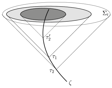
Figure 5: We call “retarded” the force (4.20) with integration over the portion of the world line before $\tau_{1}$. We call “advanced” the force (4.21) with integration over the portion of the world line after $\tau_{1}$. For an observer placed at point $z(\tau_{1})\in\zeta$ the radiative (5) and the bound (5.8) parts of massive scalar field momentum looks as the combination of incoming and outgoing radiation, and yet the retarded causality is not violated. We still consider the interference of outgoing waves presented at the observation instant $\tau$. The scalar field carries information about the charge’s past.

The support of the advanced force is a portion of the world line that corresponds to finite time interval. It is presented implicitly in the Detweiler and Whiting construction where the tail term (1.6) is introduced to achieve appropriate retarded causality. It “evaporates” in the coincidence limit $x\to z(\tau)$ at which its support $[\tau^{\rm ret}(x),\tau^{\rm adv}(x)]$ shrinks to zero.

The one-half sum of the retarded and the advanced works is the bound part of tail energy-momentum which is permanently attached to the charge and is carried along with it. It modifies particle’s individual characteristics (its momentum and its inertial mass). A point source together with surrounded “cloud” constitute dressed charged particle.

Since the properties of the retarded and the advanced solutions of wave equation, the one-half sum is singular while one-half difference is regular at the location of the particle.

The bound and the radiative angular momentum carried by charge’s field are simply torques of the above combinations of the retarded and the advanced tail forces.

Together with contributions from the direct part of Green’s function, the tail terms constitute Noether quantities removing by outgoing waves from the dressed source. Changes in individual momentum and angular momentum of dressed charged particle compensate losses of energy, momentum, and angular momentum due to radiation. (Influence of an external device can be modelled easily.) Analysis of balance equations yields the Harish-Chandra equation of motion of radiating scalar pole [13]. This equation includes the effect of particle’s own field as well as the influence of an external force.

Energy-momentum and angular momentum balance equations for radiating scalar pole constitute system of ten linear algebraic equations in variables $p^{\mu}_{\rm part}(\tau)$ and their first time derivatives ${\dot{p}}^{\mu}_{\rm part}(\tau)$ as functions of particle’s individual characteristics (velocity, acceleration, charge etc.). The system is degenerate, so that solution for particle’s 4-momentum includes arbitrary scalar function, $m(\tau)$, which can be identified with the dynamical mass of the particle. Besides renormalization constant, the mass includes contributions from particle’s own field as well as from an external field.

This is a special feature of the self force problem for a scalar charge. Indeed, the time-varying mass arises also in the radiation reaction for a pointlike particle coupled to a massless scalar field on a curved background [4]. The phenomenon of mass loss by scalar charge is studied in [29, 30]. Similar phenomenon occurs in the theory which describe a point-like charge coupled with massless scalar field in flat spacetime of three dimensions [31]. The charge loses its mass through the emission of monopole radiation.

References

• [1] B. S. DeWitt and R. W. Brehme, Ann.Phys. (N.Y.) 9, 220 (1960).
• [2] J. M. Hobbs, Ann.Phys. (N.Y.) 47, 141 (1968).
• [3] Y. Mino, M. Sasaki, and T. Tanaka, Phys. Rev. D 55, 3457 (1997).
• [4] T. C. Quinn, Phys. Rev. D 62, 064029 (2000).
• [5] E. Poisson, Living Rev. Relativity 7, Irr-2004-6 (2004). arXiv:gr-qc/0306052
• [6] S. Detweiler and B.F. Whiting, Phys. Rev. D 67, 024025 (2003).
• [7] P.A.M. Dirac, Proc. R. Soc. A (London) 167, 148 (1938).
• [8] C. Teitelboim, Phys. Rev. D 1, 1572 (1970).
• [9] Yu. Yaremko, J. Math. Phys. 48, 092901 (2007).
• [10] Yu. Yaremko, J.Phys.A: Math.Theor. 40, 13161 (2007).
• [11] D. V. Gal’tsov, Phys. Rev. D 66, 025016 (2002).
• [12] P. O. Kazinski, S. L. Lyakhovich, and A. A. Sharapov, Phys. Rev. D 66, 025017 (2002).
• [13] Harish-Chandra, Proc. R. Soc. (London) A185, 269 (1946).
• [14] B. Kosyakov, Introduction to the classical theory of particles and fields (Springer, Heidelberg, 2007).
• [15] P. Havas, Phys. Rev. 87, 309 (1952).
• [16] A. O. Barut and D. Villarroel, J. Phys. A: Math. Gen. 8, 156 (1975).
• [17] H. J. Bhabha, Proc. R. Soc. (London) A172, 384 (1939).
• [18] R. G. Cawley and E. Marx, Int. J. Theor. Phys. 1, 153 (1968).
• [19] Rohrlich F., Classical Charged Particles (Addison-Wesley, Redwood, CA, 1990).
• [20] R. G. Cawley, Ann. Phys., NY 54, 122 (1969).
• [21] R. G. Cawley, J. Math. Phys. 11, 761 (1970).
• [22] C. A. López and D. Villarroel, Phys. Rev. D 11, 2724 (1975).
• [23] E. Poisson, An introduction to the Lorentz-Dirac equation, arXiv:gr-qc/9912045 (1999).
• [24] Yu. Yaremko, J.Phys.A: Math.Gen. 36, 5149 (2003).
• [25] Yu. Yaremko, J.Phys.A: Math.Gen. 37, 1079 (2004).
• [26] F. R. Jr. Crownfield and P. Havas, Phys. Rev. 94, 471 (1954).
• [27] H.J. Bhabha and Harish-Chandra, Proc. R. Soc. (London) A183, 134 (1944).
• [28] H. J. Bhabha and Harish-Chandra, Proc. R. Soc. (London) A185, 250 (1946).
• [29] L. M. Burko, A. I. Harte, and E. Poisson, Phys. Rev. D 65, 124006 (2002).
• [30] R. Haas and E. Poisson, Class. Quantum Grav. 22, S739 (2005).
• [31] L. M. Burko, Class. Quantum Grav. 19, 3745 (2002).