Supernova-Triggered Molecular Cloud Core Collapse and the Rayleigh-Taylor Fingers that Polluted the Solar Nebula

Abstract

A supernova is a likely source of short-lived radioisotopes (SLRIs) that were present during the formation of the earliest solar system solids. A suitably thin and dense supernova shock wave may be capable of triggering the self-gravitational collapse of a molecular cloud core while simultaneously injecting SLRIs. Axisymmetric hydrodynamics models have shown that this injection occurs through a number of Rayleigh-Taylor (RT) rings. Here we use the FLASH adaptive mesh refinement (AMR) hydrodynamics code to calculate the first fully three dimensional (3D) models of the triggering and injection process. The axisymmetric RT rings become RT fingers in 3D. While $\sim 100$ RT fingers appear early in the 3D models, only a few RT fingers are likely to impact the densest portion of the collapsing cloud core. These few RT fingers must then be the source of any SLRI spatial heterogeneity in the solar nebula inferred from isotopic analyses of chondritic meteorites. The models show that SLRI injection efficiencies from a supernova several pc away fall at the lower end of the range estimated for matching SLRI abundances, perhaps putting them more into agreement with recent reassessments of the level of ⁶⁰Fe present in the solar nebula.

1 Introduction

Chondritic meteorites contain daughter products of the decay of short-lived radioisotopes (SLRIs), such as ²⁶Al (Lee et al. 1976; Amelin et al. 2002) and ⁶⁰Fe (Tachibana & Huss 2003), present during the formation of the earliest solids in the solar system. Recent evidence has raised doubts about the initial amount of ⁶⁰Fe present in the solar nebula. Moynier et al. (2011) presented evidence for an initial ratio of ⁶⁰Fe/⁵⁶Fe less than $3\times 10^{-9}$, roughly 100 times smaller than previously published ratios (e.g., Mishra et al. 2010), while Tang & Dauphas (2012) found an initial ratio of $1\times 10^{-8}$. The initial level of ⁶⁰Fe is particularly significant, as its efficient production requires stellar nucleosynthesis (Tachibana et al. 2006) in either a massive star supernova or an AGB star (Huss et al. 2009). If the initial level of ⁶⁰Fe is low enough, cosmic rays may be sufficient to create this SLRI (Moynier et al. 2011). The interstellar medium (ISM) appears to have ⁶⁰Fe/⁵⁶Fe = $1\times 10^{-7}$ (Tang & Dauphas 2012), implying that lower ratios could be inherited from the ISM after a suitable decay interval (e.g., Gounelle et al. 2009; Tang & Dauphas 2012). While the initial ⁶⁰Fe/⁵⁶Fe ratio is uncertain, other recent studies have shown that this ratio appears to be $\sim 2\times 10^{-7}$ for certain chondrules found in unequilibrated ordinary chondrites (Telus et al. 2012). Such ratios may require a stellar nucleosynthetic source for this SLRI.

Boss et al. (2010) used the FLASH AMR code to study presolar cloud core triggering and injection processes associated with SLRI production in either a core collapse supernova or an AGB star. They showed that shock waves from a supernova or an AGB star could simultaneously trigger the collapse of a dense molecular cloud core and inject shock wave material into the resulting protostar. Boss & Keiser (2010, hereafter BK10) found, however, that the injection efficiency depended sensitively on the assumed shock width and density. Supernova shock waves appeared to be thin enough to inject the desired amount of shock wave material. Planetary nebula shock waves, derived from AGB star winds, however, were too thick to achieve the desired injection efficiencies. BK10 thus concluded that a supernova was the likely trigger for solar system formation, a conclusion that has been supported by subsequent theoretical (Gritschneder et al. 2012), observational (e.g., Diehl et al. 2010; Phillips & Marquez-Lugo 2010), and cosmochemical studies (e.g., Young et al. 2011; Krot et al. 2012). Other scenarios are reviewed by Adams (2010) and Boss (2012).

2 Numerical Methods and Initial Conditions

Here we extend the BK10 2D AMR models to fully 3D AMR calculations using the 3D Cartesian coordinate ($x,y,z$) version of FLASH2.5 in much the same manner as our previous calculations with the axisymmetric ($R$, $Z$) version. The grid was 0.2 pc long in $y$ (the direction along which the shock wave travels initially) and 0.13 pc wide in $x$ and $z$. The target cloud is a Bonnor-Ebert sphere with a central density of $1.24\times 10^{-18}$ g cm^-3, a radius of 0.058 pc, and a mass of 3.8 $M_{\odot}$, initially centered on the grid at $x=z=0$ and $y=$ 0.13 pc. The cloud is composed of molecular hydrogen gas with a mean molecular weight $\mu=2.3$. The initial number of blocks in $x$ and $z$ was 6 and in $y$ was 9, with each block consisting of $8^{3}$ grid points. The number of levels of grid refinement was initially 4, but was increased to as high as 7 levels (when possible) to better resolve the protostellar core, leading to effective resolutions as high as $3072^{3}$ in regions with large gradients in the density or color (shock front) fields. A typical simulation ran for three months on the dedicated flash cluster at DTM.

The initial shock parameters (Table 1) overlap with those of BK10, where the standard shock number density was $n_{s}=10^{4}$ cm^-3 and shock width was $w_{s}=10^{16}$ cm. Model 40-400-0.1 has $v_{s}=$ 40 km/sec, shock number density $n_{s}=4\times 10^{6}$ cm^-3, and shock width $w_{s}=10^{15}$ cm. The post-shock density $n_{s}$ for an isothermal shock in a gas of density $n_{m}$ is $n_{s}/n_{m}=(v_{s}/c_{m})^{2}$, where $c_{m}$ is the pre-shock sound speed. For our 40 km/sec models, with $c_{m}=0.2$ km/sec and $n_{m}=10^{2}$ cm^-3, $n_{s}=4\times 10^{6}$ cm^-3, the same density as in model 40-400-0.1. For comparison, W44 is a Type II supernova remnant (SNR) with $v_{s}=20-30$ km/sec, width $<10^{16}$ cm, and radius $\sim 11$ pc, expanding into gas with $n\sim 10^{2}$ cm^-3 (Reach et al. 2005).

As in BK10, we included compressional heating and radiative cooling, based on the results of Neufeld & Kaufman (1993) for cooling caused by rotational and vibrational transitions of optically thin, warm molecular gas composed of H₂O, CO, and H₂, leading to a radiative cooling rate of $\Lambda\approx 9\times 10^{19}(T/100)\rho^{2}$ erg cm^-3 s^-1, where $T$ is the gas temperature in K and $\rho$ is the gas density in g cm^-3.

3 Results

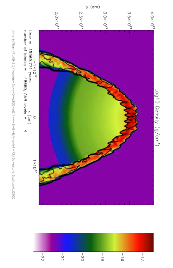
Figure 1: Log10 of the density distribution for model 40-200-0.1 after $2.00\times 10^{4}$ yrs of evolution, plotted in the $z=0$ plane. Contours show the color field plotted at 0.01, 0.025, 0.05, 0.075, and 0.1. The $x$ axis is horizontal and the $y$ axis is vertical. The downward propagating shock wave has compressed the target cloud core and is injecting shock front material through multiple Rayleigh-Taylor (RT) fingers.

The overall evolution of the 3D AMR models proceeds in a manner very similar to that of the 2D AMR models of Boss et al. (2008, 2010) and BK10: the shock wave strikes the target cloud core, compressing the facing edge of the cloud, as the shock wave propagates unimpeded around the sides of the cloud, forming a parabolic shock front. Figure 1 shows a cross-section through model 40-200-0.1 after 0.02 Myr of evolution, when the cloud core has been compressed by a factor of $\sim$ 30 by a shock initially propagating downwards (toward $y=0$). Model 40-200-0.1 has $v_{s}=$ 40 km/sec, $\rho_{s}$ = $7.2\times 10^{-18}$ g cm^-3 (200 times the standard density), and $w_{s}=$ 0.0003 pc (0.1 times the standard width). Figure 1 shows that the color field, representing the shock wave material, has been injected into the shock-compressed outer cloud layers. The shock corrugates the surface of the compressed cloud core with a series of indentations indicative of a Rayleigh-Taylor (RT) instability. Meanwhile, Kelvin-Helmholtz (KH) instabilities caused by velocity shear form in the relatively unimpeded portions of the shock front at large impact parameter compared to the center of the target cloud. The shock front gas and dust is entrained and injected into the compressed region by the RT instability, while the KH rolls result in ablation and loss of target cloud mass in the downstream flow.

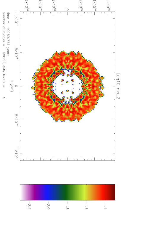
Figure 2: Log10 of the color field distribution for model 40-200-0.1 after $2.00\times 10^{4}$ yrs of evolution, plotted in the $y=0.11$ pc plane. The $x$ axis is horizontal and the $z$ axis is vertical. Roughly 100 RT fingers are evident as the shock front material is injected into the target cloud core.

Figure 1 shows that in 3D, the initially high symmetrical configuration remains fairly axisymmetrical. The number of RT fingers evident in the cross section at this time is $\sim 16$, the same number of fingers (assuming axisymmetry) as seen in the corresponding BK10 2D AMR model, and with a very similar spacing and distribution across the shock/cloud interface. The main difference is that the 2D RT structures are rings, not fingers. While we have not performed a convergence study (e.g., Pittard et al. 2009; Yirak et al. 2010), the fact that the 2D model has nearly four times the spatial resolution in each direction as the 3D model, yet yields the same number of R-T features, implies a reasonable degree of numerical convergence. Figure 2 shows a cross-section in the direction perpendicular to that of the shock wave propagation (i.e., in the $x$ - $z$ plane), which clearly exhibits the formation of numerous ($\sim$ 100) distinct RT fingers in the shock wave matter.

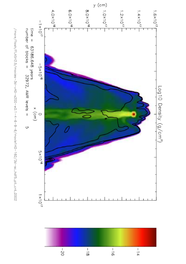
Figure 3: Log10 of the density distribution and color field (SLRIs) contours (plotted in linear steps of 0.01) for model 40-200-0.1 after $6.32\times 10^{4}$ yrs of evolution, plotted as in Figure 1. The cloud core has been driven into dynamic collapse by the shock front, and has formed a well-defined, high density, collapsing protostar with a radius of $\sim$ 100 AU.

Figure 3 shows model 40-200-0.1 after 0.063 Myr of evolution, when the cloud core has been compressed to a maximum density over $10^{5}$ times higher than the initial maximum density: the cloud core is dynamically collapsing with a radius of order 100 AU. As in 2D, by this time the color field has been injected throughout the collapsing region, though with varying color field density. The mass of the collapsing protostar is roughly $1M_{\odot}$, with a maximum density at this time of $\sim 2\times 10^{-13}$ g cm^-3, high enough to enter the regime of protostellar collapse when the collapsing cloud core becomes optically thick in the infrared, and our assumption of optically thin, radiative cooling begins to fail.

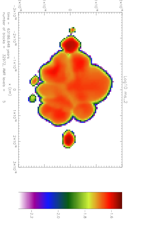
Figure 4: Log10 of the color field distribution for model 40-200-0.1 after $6.32\times 10^{4}$ yrs of evolution, plotted as in Figure 2, but in the $y=0.045$ pc plane. Given the 2666 AU width of this plot, and the $\sim 100$ AU size of the protostar (Figure 3) at this time, it is likely that only one (or at most a few) RT fingers will be responsible for most of the shock wave injection into the collapsing presolar cloud core.

Figure 4 shows the status of the RT fingers at the same time (0.063 Myr) as Figure 3, displayed again in the $x-z$ plane, so that the number of RT fingers can be counted. Figure 4 is plotted for $y=0.045$ pc = $1.4\times 10^{17}$ cm, at a height just above the protostellar object seen in Figure 3. Figure 4 shows that the 100-odd RT fingers evident in Figure 2 have been reduced to about 10, largely due to the ablation of target cloud mass into the downstream flow. Figure 4 shows that only a limited number of RT fingers will inject SLRIs. In fact, given that the radius of the protostar at this time is $\sim$ 100 AU $\sim 10^{15}$ cm, Figure 4 shows that it is possible that a single RT finger, the one at the center, will successfully inject shock wave material into the protostar. The remaining RT fingers will likely continue downstream past the collapsing protostar. This reduction in the number of RT fingers responsible for injection also appears to be due in part to merging of the fingers, as Figure 4 shows that the RT fingers are less distinct than in Figure 2. A similar effect can be seen in the high resolution 2D models of Vanhala & Boss (2002): the number of distinct RT rings decreases from $\sim$ 12 at 0.022 Myr to $\sim$ 4 at 0.13 Myr.

With the exception of model 40-800-0.1, where the shock-compressed shell was shredded and did not undergo collapse, all the other models listed in Table 1 evolved in a manner similar to that of model 40-200-0.1 and displayed in the four figures. The result for model 40-800-0.1 was to be expected, as the same model failed to undergo sustained collapse when calculated in 2D by BK10. It is reassuring, however, to obtain the same result when re-calculated in 3D, as the implication is that 2D models can be used to survey a larger parameter space than can be explored with 3D models.

4 Injection Efficiency and Dilution Factors

For comparison to isotopic analyses of primitive meteorites, we must estimate injection efficiencies and dilution factors. We assume that the SLRIs are carried by dust grains that are small enough to move along with the gas, as calculated by the AMR code. The injection efficiency $f_{i}$ is defined to be the fraction of the incident shock wave material that is injected into the collapsing cloud core. The factor $\beta$ is the ratio of shock front mass originating in the SN to the mass swept up in the intervening ISM. The dilution factor $D$ is then defined as the ratio of the amount of mass derived from the supernova to the amount of mass derived from the target cloud. The portion of the shock front in model 40-200-0.1 incident on the cloud contains 0.3 $M_{\odot}$ of gas and dust, implying $D\approx 0.3\beta f_{i}$, for a final system mass of 1 $M_{\odot}$. This assumes that the injected SLRIs are uniformly distributed in the collapsing cloud core, as well as in the resulting protostar and protoplanetary disk.

Estimates of the injection efficiency $f_{i}$ are made difficult by the fact that by the time that the calculations are halted because of the rising optical depth, the protostar is still far from having formed a well-defined young stellar object and protoplanetary disk. Hence the exact amount of shock front matter that is incorporated into the protostar is uncertain, as it will be a combination of the matter already injected into the collapsing region and that accreted at a later time. Given this uncertainty, the injection efficiencies for the 3D models appear to be similar to those of the corresponding BK10 2D models: the color field densities in the collapsing region of the 40 km/sec shock model 200-0.1 (BK10’s Figure 4) are very similar ($\sim 0.03$ in dimensionless units, compared to an initial color density of 1) to that of model 40-200-0.1 at the time shown in Figures 3 and 4.

For model 40-200-0.1, assuming that a region around the collapsing protostar seen in Figure 3 with a radius of $\sim 10^{16}$ cm is eventually accreted by the protostar, the injection efficiency $f_{i}\sim 0.03$, close to the BK10 estimate of $f_{i}\sim 0.02$. With this new estimate for $f_{i}$, we find $D\sim 0.01\beta$. In order for a supernova shock to slow down to a speed of 40 km/sec, however, a considerable amount of ISM matter must be snowplowed by the shock front, reducing $D$ by a factor of $\beta\sim 0.01$ to $D\sim 10^{-4}$, for a shock that travels $\sim 5$ pc from a 20 $M_{\oplus}$ SN (e.g., Ouellette et al. 2007) through an ISM with $n\sim 10^{2}$ cm^-3. This estimate falls at the low end of the range of dilution factors inferred for typical SLRIs from SN, namely $\sim 10^{-4}$ to $\sim 3\times 10^{-3}$ (Takigawa et al. 2008; Gaidos et al. 2009).

Several other factors, however, could result in increased values of $D$, such as enhanced mixing associated with sub-grid turbulence (Pittard et al. 2009), preferential addition of the SLRIs to the disk rather than the protostar (BK10), and enhanced injection of the SLRIs through their presence in dust grains large enough to punch through the shock-cloud interface more effectively than gaseous RT fingers (BK10). While investigation of the intermediate scenario will require calculations of rotating target clouds, so that protoplanetary disks can form, the latter scenario can be evaluated now. The core-collapse supernova 1987A, e.g., appears to have produced a dust mass of about 0.4 to 0.7 $M_{\odot}$ (Matsuura et al. 2011), and these dust grains presumably carry the freshly synthesized SLRIs.

BK10 estimated that dust grains larger than $\sim 30\mu$m would be needed in order to increase $D$ values. However, dust grains in SNRs are thought to be smaller than $\sim 30\mu$m. Nozawa et al. (2010) found an average radius of dust grains less than 0.01 $\mu$m for the Cas A SNR of a Type IIb SN. Andersen et al. (2011) fit the spectral energy distributions of 14 SNRs with several different populations of dust grains, where the largest grains needed were smaller than 0.1 $\mu$m. In their models of dust processing in C-type shocks, appropriate for SNRs, Guillet et al. (2011) considered dust grains all smaller than 0.03 $\mu$m. Hence dust grains in SNRs do not appear to be large enough to result in significantly enhanced injection efficiencies. Another constraint comes from presolar dust grains, derived from a variety of stellar outflows, such as SN (e.g., Amari et al. 1994) and AGB stars (e.g., Bernatowicz et al. 2006), some of which can be 6 $\mu$m in size. However, only about 1% of these grains are larger than 1 $\mu$m. We conclude that SLRIs carried by large dust grains are insufficient to raise the injection efficiencies significantly.

We are left, however, with another means of reconciling the dilution factors estimated on the basis of these 3D models ($D\sim 10^{-4}$) with those inferred from a combination of SN nucleosynthesis abundance calculations and laboratory analysis of primitive meteorites, which have been as high as $\sim$ 30 times larger (Takigawa et al. 2008; Gaidos et al. 2009). The production amounts of SLRI such as ²⁶Al and ⁶⁰Fe in core-collapse supernovae appear to be uncertain by factors of five or more (Tur et al. 2010). In addition, the fact that recent estimates of the initial ⁶⁰Fe abundance in the solar nebula have fallen considerably, in some cases by factors of 100 or more (Moynier et al. 2011), suggests that it may well be possible to accommodate the supernova triggering and injection scenario for the origin of the solar nebula’s SLRIs. ⁶⁰Fe seems to be the key SLRI, as ²⁶Al is relatively abundant in the interstellar medium (e.g., Diehl et al. 2010) and is expected to be concentrated in the outflows of Wolf-Rayet stars that are the predecessors to many Type II SN (Tatischeff, Duprat, & de Séréville 2010). AGB stars, however, still appear to be ruled out, on the basis of the even lower injection efficiencies resulting from the much thicker width of planetary nebula outflows compared to SNRs (BK10).

5 Conclusions

While supernova triggering and injection is a possible explanation of the evidence for SLRIs in meteorites, it remains to be seen if a combination of target cloud and shock front parameters can be found that will produce the correct SLRI injection efficiencies and also be consistent with observations of SNRs. Assuming the suitability of our shock front parameters, the 3D models show that a relatively small number of RT fingers are likely to have been involved in the injection of the SNR SLRIs into the solar nebula, which has significant consequences for the processes of mixing and transport that occurred after injection into the nebula (e.g., Boss 2011) and for the resulting levels of isotopic homogeneity and heterogeneity (e.g., Bouvier & Wadhwa 2010; Schiller et al. 2010; Larsen et al. 2011; Makide et al. 2011; Wang et al. 2011; Boss 2012). Furthermore, our estimates of injection efficiencies and dilution factors will become important discriminators for judging the likelihood of the supernova triggering and injection scenario once a clearer picture emerges of the initial abundances of the SLRIs (principally ⁶⁰Fe: Moynier et al. 2011; Telus et al. 2012) that were present during the formation of the various components of the most primitive meteorites.

Table 1: Initial parameters explored for the 3D AMR models, showing the outcomes for models with varied initial shock speeds ($v_{s}$, in km/sec), shock density ($\rho_{s}$, in units of the standard density of $3.6\times 10^{-20}$ g cm^-3), and shock width ($w_{s}$, in units of the standard width of 0.003 pc). The outcomes are listed as C for sustained collapse and NC for no sustained collapse.

shock density $\times$		1	200	400	800	1000	1600
shock width $\times$ 1	$v_{s}=$ 20	C	-	-	-	-	-
shock width $\times$ 0.1	$v_{s}=$ 20	-	C	C	C	C	C
shock width $\times$ 1	$v_{s}=$ 40	C	-	-	-	-	-
shock width $\times$ 0.1	$v_{s}=$ 40	-	C	C	NC	-	-

References

- (1)
- (2) Adams, F. C. 2010, ARA&A, 48, 47
- (3)
- (4) Amari, S., Lewis, R. S., & Anders, E. 1994, Geochim. Cosmochim. Acta, 58, 459
- (5)
- (6) Amelin, Y., Krot, A. N., Hutcheon, I. D., & Ulyanov, A. A. 2002, Science, 297, 1678
- (7)
- (8) Andersen, M., Rho, J., Reach, W. T., Hewitt, J. W., & Bernard, J. P. 2011, ApJ, 742, 7
- (9)
- (10) Bernatowicz, T. J., Croat, T. K., & Daulton, T. L. 2006, in Meteorites and the Early Solar System II, ed. D. S. Lauretta & H. Y. McSween (Tucson, AZ: Univ. Arizona Press), 109
- (11)
- (12) Bonnor, W. B. 1956, MNRAS, 116, 351
- (13)
- (14) Boss, A. P. 2011, ApJ, 739, 61
- (15)
- (16) Boss, A. P. 2012, ARE&PS, 40, 23
- (17)
- (18) Boss, A. P., & Keiser, S. A. 2010, ApJ, 717, L1
- (19)
- (20) Boss, A. P. et al. 2008, ApJ, 686, L119
- (21)
- (22) Boss, A. P. et al. 2010, ApJ, 708, 1268
- (23)
- (24) Bouvier, A., & Wadhwa, M. 2010, Nature Geoscience, 3, 637
- (25)
- (26) Diehl, R., et al. 2010, A&A, 522, A51
- (27)
- (28) Gaidos, E., Krot, A. N., Williams, J. P., & Raymond, S. N. 2009, ApJ, 696, 1854
- (29)
- (30) Gritschneder, M., Lin, D. N. C., Murray, S. D., Yin, Q.-Z., & Gong, M.-N. 2012, ApJ, 745, 22
- (31)
- (32) Guillet, V., Pineau des Forêts, G., & Jones, A. P. 2011, A&A, 527, A123
- (33)
- (34) Gounelle, M., Meibom, A., Hennebelle, P., & Inutsuka, S.-I. 2009, ApJ, 694, L1
- (35)
- (36) Huss, G. R., et al. 2009, Geochim. Cosmochim. Acta, 73, 4922
- (37)
- (38) Krot, A. N., et al. 2012, 43rd Lunar Planet. Sci. Conf., #2255
- (39)
- (40) Larsen, K. K., et al. 2011, ApJL, 735, L37
- (41)
- (42) Lee, T., Papanastassiou, D. A., & Wasserburg, G. J. 1976, Geophys. Res. Lett., 3, 41
- (43)
- (44) Makide, K., et al. 2011, ApJL, 733, L31
- (45)
- (46) Matsuura, M., et al. 2011, Science, 333, 1258
- (47)
- (48) Mishra, R. K., Goswami, J. N., Tachibana, S., Huss, G. R., & Rudraswami 2010, ApJL, 714, L217
- (49)
- (50) Moynier, F., Blichert-Toft, J., Wang, K., Herzog, G. F., & Albarede, F. 2011, ApJ, 741, 71
- (51)
- (52) Neufeld, D. A., & Kaufman, M. J. 1993, ApJ, 418, 263
- (53)
- (54) Nozawa, T., et al. 2010, ApJ, 713, 356
- (55)
- (56) Ouellette, N., Desch, S. J., & Hester, J. J. 2007, ApJ, 662, 1268
- (57)
- (58) Phillips, J. P., & Marquez-Lugo, R. A. 2010, MNRAS, 409, 701
- (59)
- (60) Pittard, J. M., Falle, S. A. E. G., Hartquist, T. W., & Dyson, J. E. 2009, MNRAS, 394, 1351
- (61)
- (62) Reach, W. T., Rho, J., & Jarrett, T. H. 2005, ApJ, 618, 297
- (63)
- (64) Schiller, M., Handler, M. R., & Baker, J. A. 2010, Earth Planet. Sci. Lett., 297, 165
- (65)
- (66) Tachibana, S., & Huss, G. R. 2003, ApJ, 588, L41
- (67)
- (68) Tachibana, S., et al. 2006, ApJ, 639, L87
- (69)
- (70) Takigawa, A., et al. 2008, ApJ, 688, 1382
- (71)
- (72) Tang, H., & Dauphas, N. 2012, 43rd Lunar Planet. Sci. Conf., #1703
- (73)
- (74) Tatischeff, V., Duprat, J., & de Séréville, N. 2010, ApJL, 714, L26
- (75)
- (76) Telus, M., Huss, G. R., Nagashima, K., Ogliore, R. C., & Tachibana, S. 2012, 43rd Lunar Planet. Sci. Conf., #2733
- (77)
- (78) Tur, C., Heger, A., & Austin, S. M. 2010, ApJ, 718, 357
- (79)
- (80) Vanhala, H. A. T., & Boss, A. P. 2002, ApJ, 575, 1144
- (81)
- (82) Wang, K., Moynier, F., Podosek, F., & Foriel, J. 2011, ApJL, 739, L58
- (83)
- (84) Yirak, K., Frank, A., & Cunningham, A. J. 2010, ApJ, 722, 412
- (85)
- (86) Young, E. D., Gounelle, M., Smith, R. L., Morris, M. R., & Pontoppidan, K. M. 2011, ApJ, 729, 43
- (87)