EMRI data analysis with a phenomenological waveform

Abstract

Extreme mass ratio inspirals (EMRIs) (capture and inspiral of a compact stellar mass object into a Massive Black Hole (MBH)) are among the most interesting objects for the gravitational wave astronomy. It is a very challenging task to detect those sources with the accurate estimation parameters of binaries primarily due to a large number of the secondary maxima on the likelihood surface. Search algorithms based on the matched filtering require computation of the gravitational waveform hundreds of thousands of times, which is currently not feasible with the most accurate (faithful) models of EMRIs. Here we propose to use a phenomenological template family which covers a large range of EMRIs parameter space. We use these phenomenological templates to detect the signal in the simulated data and then, assuming a particular EMRI model, estimate the physical parameters of the binary. We have separated the detection problem, which is done in a model-independent way, from the parameter estimation. For the latter one, we need to adopt the model for inspiral in order to map phenomenological parameters onto the physical parameter characterizing EMRIs.

I Introduction

Stellar compact objects like a black hole, neutron star or white dwarf in the cusp surrounding the massive black hole (MBH) in the galactic nuclei could be deployed on a very eccentric orbit due to N-body interaction. Such an object could either plunge (directly or after few orbits) into MBH or form an EMRI: inspiralling compact object on originally very eccentric orbit which shrinks and circularizes due to loss of the energy and angular orbital momentum through gravitational radiation. The compact object spends $\sim 10^{6}$ orbits in the very strong field of a MBH before it plunges, all this orbital evolution will be encoded in the phase of emitted gravitational waves (GWs). Space based GW observatories, like LISA or similar planned missions, will observe those sources few years before the plunge. By fitting precisely the GW phase one can extract extremely accurate parameters of a binary system Barack:2003fp (like mass and spin of MBH $M,a$, mass of a small object $m$, inclination of the orbital plane (to the spin of MBH), orbital eccentricity and semi-latus rectum ($\iota_{0},e_{0},p_{0}$) at some fiducial moment of time $t_{0}$, location of the source on the sky ($\theta,\phi$) and more).

Precise tracking of the GW phase implies that we can also test the nature of the central massive object. The general belief is that it should be a MBH with surrounding spacetime described by a Kerr solution. The nature of the spacetime affects the orbital evolution of the compact object which in turn could be extracted from the GW phase. Kerr spacetime is described by only two parameters: black hole’s mass and spin, as stated by a “no-hair” theorem. The spacetime could be decomposed in the multipole moments of a central massive object, and, for Kerr BH, all moments depend only on $M$ and $a$: $M_{l}+iS_{l}=(ia)^{l}M^{l+1}$ where $M_{l}$ and $S_{l}$ are mass and current moments. We could measure three first moments (mass, spin and quadrupole moment)Barack:2006pq , and check the “Kerrness” of a spacetime. In general, the deviations from Kerr could come in several ways: (i) it is Kerr BH but there is an additional perturber (gas disk, another MBH) (ii) it is not Kerr BH but some other object satisfying GR (boson star, gravastar), (iii) there are deviations from GR. For discussion on the topics we refer the reader to Babak:2010ej ; AmaroSeoane:2010zy ; AmaroSeoane:2012je and references therein.

Modeling orbital evolution even within GR is not yet fully complete. Large mass ratio allows us to consider a small compact object as a perturbation on the Kerr background spacetime, and treat the problem perturbatively in orders of the mass ratio. In zero order approximation the compact object moves on a geodesic orbit, however, as soon as we assign the mass to it, it creates its own gravitational field interacting with the background and this system emits gravitational radiation. The force resulting from the interaction of the self field with the background is called self force, and the motion of the compact object could be seen as the forced geodesic motion. Alternative interpretation is that the motion is governed by a geodesic motion but in the perturbed spacetime. Calculation of the self force is a complicated task which is accomplished for the orbits around Schwarzschild BH only Warburton:2011fk ; Barack:2010tm , the Kerr spacetime is underway. There are also questions concerning the calculation of the orbital evolution under the self force: the self force depends on the past history of the compact object (which is usually assumed to be a geodesic in the background spacetime). To compute the motion under the self force one can use the osculating elements approach Gair:2010iv , or self-consistent approach of direct integration of the regularized equations Diener:2011cc . For more details on this subject we refer to lrr-2011-7 .

All in all, the modeling of the orbital evolution and the GW signal is a complex task which requires significant theoretical and computational developments. The latter prevents us currently from using the state-of-art GW models of EMRIs in our data analysis explorations. In majority of the cases the phenomenological model suggested in Barack:2003fp , so called “analytic kludge” (AK), is used. It is based on Post-Newtonian expressions and puts together all relevant physics of EMRIs. However, this model has restrictions in the number of harmonics and in their strength, and any search algorithm which relies on its specific harmonic content will not work for a more realistic model of GW signal. The main motivation of this work is to create the phenomenological search template family which would fit a very large range of EMRI-like signals. The typical EMRI signal consists of a set of harmonics of three (slowly evolving) orbital frequencies, and we will use it as a basis of our template. The phenomenological template consists of $N_{h}$ harmonics with constant amplitude and slowly evolving phase which we decompose in a Taylor series. Truncation of the Taylor series and the assumption about constant amplitude set restrictions on the duration over which the phenomenological template can fit an EMRI signal. The amplitude of EMRI’s harmonics changes due to shrinking of the orbit (overall amplitude increases), circularization of the orbit (power is shifted to lower harmonics) and slight change in the inclination of the orbit to the spin of MBH. Using more terms in the Taylor series helps to track phase of the EMRI signal for longer time (which is more important than accurate description of the amplitude). Finally, we decide on the number of harmonics to use in the template (and their indices) based on the analysis of the harmonic structure of the Numerical Kludge (NK) model Babak:2006uv of EMRI in different parts of the parameter space. The restriction that the phenomenological waveform (PW) is valid only for a limited period of time is very weak since we can fit the signal piecewise, as long as the accumulated signal-to-noise ratio (SNR) over that time is significant to claim presence of the signal. In this work we consider only those parts of the EMRI signal where the orbital frequencies are not decreasing which is true over almost all time of the inspiral and breaks quite close to the plunge. However, this is not really necessary since we did not restrict the values of frequency derivatives to positive values during the search.

The PW family is quite generic and does not depend on the orbital evolution, or, in other words, the orbital evolution of the binary is encoded in the Taylor coefficients of phase of each harmonic. This allows us to detect an EMRI signal in a model independent way. Once the harmonics of the signal are recovered we can analyze them using a specific EMRI model to recover physical parameters of the system. It is at this point we need the orbital evolution with high accuracy, which involves computation of the self-force and tests of possible deviations from the “Kerrness”.

After constructing the phenomenological waveform we perform blind searches on the simulated data without noise (to avoid stochastic errors in the parameter estimation) and with the noise. We have used the NK waveform (as described in Babak:2006uv ) as a model of our signal and the orbital evolution according to Gair:2005ih . We have also used Markov chain Monte-Carlo (MCMC) search with phenomenological waveforms on the simulated three month of data. This search has provided us with multiple local maxima in the likelihood which we gathered and analyzed in a similar way as described in Babak:2009ua . We associate local maxima in the likelihood with partial detections of the signal and construct the time-frequency map of the detected (patchy) harmonics of the source. The next step is to assume the model for the orbital evolution and, by matching the found time-frequency tracks to the harmonics of the signal, estimate parameters of the binary system. We have used the same model for the orbital evolution as in the simulated data sets and recovered physical parameters with precision better than few percent.

The paper is organized as follows. In the next Section we will give a brief overview of available models for GWs from EMRIs. In Section III, we introduce PW family in details. We describe MCMC search with PWs in Section IV. Analysis of MCMC results and mapping to the physical parameters are done in the Section V. Finally we conclude with a summary Section VI.

II Review of EMRI waveforms

As was already mentioned in the Introduction, accurate computation of the GWs from EMRIs and the orbital evolution is a complex and computationally intensive task. The most promising approach probably is the coupled integration of the compact object dynamics and GW emission taken in Diener:2011cc . Alternatively, one could have a separate evolution of the orbital motion using self force computed across various geodesic orbits and employ osculating elements approach Pound:2007th ; Gair:2010iv . The waveform at infinity could be obtained from the Teukolsky equations Teukolsky:1973ha in time or in frequency domain Martel:2003jj ; Drasco:2005kz .

The above methods are computationally expensive and several approximations were suggested. Less accurate but still quite reliable are Numerical Kludge (NK) waveforms: original NK Babak:2006uv and extended/improved NK called “Chimera” Sopuerta:2011te ; Sopuerta:2012de . Those methods combine accurate prescription for the orbital evolution with approximate (Post-Newtonian) waveform generation formalism.

The less precise model, which captures all relevant physics of EMRIs (orbital precession, three orbital frequencies) was suggested in Barack:2003fp , so called Analytic Kludge waveform. These waveforms are very fast to generate, and even though they cannot be used for searching for actual GW signals, they are used to develop data analysis algorithms and to evaluate their performance Barack:2003fp ; Barack:2006pq ; Babak:2009cj .

In this work, we used NK waveform. In the original paper, Babak:2006uv , the waveform was generated in the time domain, we have reimplemented it in the frequency domain following suggestions of S. Drasco who did it first (private communications). However, we still take into account the time dependence of only three orbital constants under radiation reaction: energy, azimuthal component of the orbital angular momentum and Carter constant. Under the self force in osculating element approach we should evolve also other three constants (defining initial position of the compact object) due to conservative part of the self-force Pound:2007th ; Gair:2010iv . This does not affect our search results, since PW is model independent, however, we have to use the same model (as in the simulated data) for mapping the phenomenological parameters onto the physical parameters of the binary. Mismatch in the models would result in the bias which we want to avoid.

Finally we want to avoid using in this work the Analytic Kludge model, because it predicts somewhat simplified (detectable) harmonic content of the waveform. The NK waveforms for generic orbits were compared against waveforms based on the Teukolsky equation and they show quite good agreement. We believe that NK deviates from the true EMRI signal in the phase but not so much in the number and strength of harmonics. Therefore we use NK model as a representation of the EMRI signal throughout this paper.

III EMRI phenomenological waveform family

There are several algorithms which have been proven to be successful in detecting EMRIs in the simulated LISA data Cornish:2008zd ; Babak:2009cj ; Babak:2009ua . However, those algorithms partially utilize the features of AK waveform which was used in the simulation of the data and in the data analysis. As explained in Section II, we want to avoid it by building a generic phenomenological template family.

III.1 Phenomenological waveform in the source frame

The model we want to propose is based on the following assumptions about GW signals from EMRIs:

1. The orbital motion can be effectively described by six slowly changing quantities. Explicitly, three time-dependent initial phases are governed by the conservative part of the self force; three fundamental time-dependent frequencies are governed by the radiative part of the self force.

2. The waveform is represented by harmonics of three frequencies (phenomenologically, these frequencies are the summation of the fundamental orbital frequencies and the evolution of the initial phases) with slowly changing intrinsic amplitude:

$$h(t) = \sum_{l,m,n}{h_{lmn}(t)}$$ (1)

$$= \mathrm{Re}\left(\sum_{l,m,n}{A_{lmn}(t)e^{i\Phi_{lmn}(t)}}\right)$$

$$= \mathrm{Re}\left(\sum_{l,m,n}{A_{lmn}(t)e^{i(l\Phi_{r}+m\Phi_{\theta}+n\Phi_{\varphi})}}\right),$$

where $\Phi_{r},\Phi_{\theta},\Phi_{\varphi}$ are the phase evolutions corresponding to the three fundamental motions. Here we omitted the tensorial spatial indices for simplicity.

The first assumption basically expresses that the motion is described by a slow drift from one geodesic to another. The initial phases correspond to the initial position of a compact object on a given geodesic and the orbital frequencies are functions of the energy, azimuthal component of the orbital momentum and Carter constant. The slow drift ensures that phases $\Phi_{lmn}$ are slowly varying functions of time.

Fig. 1 shows the time-frequency plot of a typical EMRI signal.There are 30 clearly separated frequency tracks in the noiseless plot, which display the dominant harmonics. It can also be seen that the frequencies of harmonics are smooth and vary slowly.

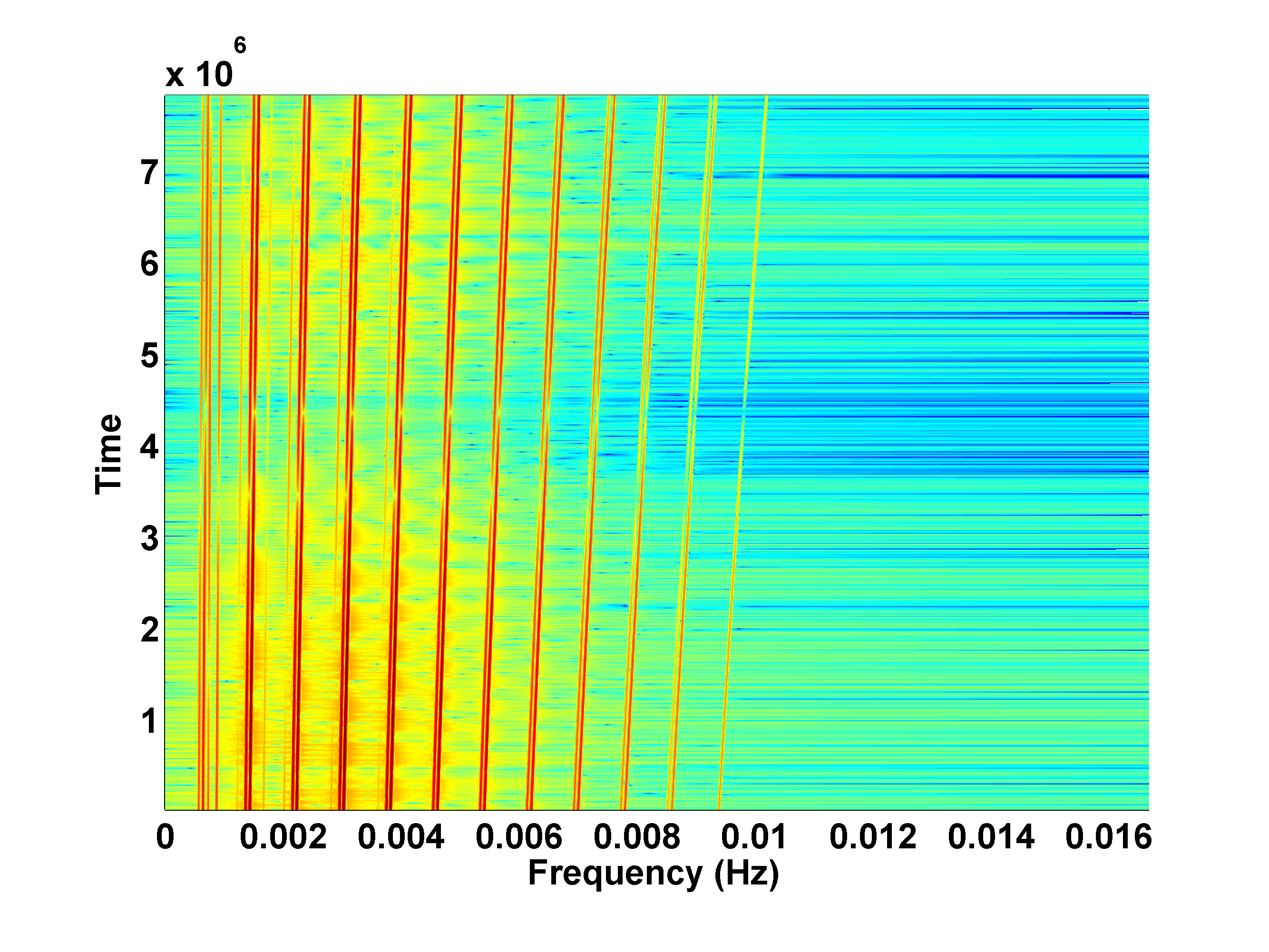
Figure 1: The time-frequency plot of a typical EMRI signal without noise. There are 30 dominant harmonics in total.

It is generally true that both amplitude and the phase are slowly varying functions of time, thus we can safely make the Taylor expansion:

$$\Phi_{r}(t) = \Phi_{r}(t_{0})+\omega_{r}(t_{0})(t-t_{0})+\frac{1}{2}\dot{\omega}_{r}(t-t_{0})^{2}+\ldots$$

$$= \Phi_{r}(t_{0})+2\pi f_{r}(t_{0})(t-t_{0})+\pi\dot{f}_{r}(t-t_{0})^{2}+\ldots,$$

$$\Phi_{\theta}(t) = \Phi_{\theta}(t_{0})+\omega_{\theta}(t_{0})(t-t_{0})+\frac{1}{2}\dot{\omega}_{\theta}(t-t_{0})^{2}+\ldots$$

$$= \Phi_{\theta}(t_{0})+2\pi f_{\theta}(t_{0})(t-t_{0})+\pi\dot{f}_{\theta}(t-t_{0})^{2}+\ldots,$$

$$\Phi_{\varphi}(t) = \Phi_{\varphi}(t_{0})+\omega_{\varphi}(t_{0})(t-t_{0})+\frac{1}{2}\dot{\omega}_{\varphi}(t-t_{0})^{2}+\ldots$$

$$= \Phi_{\varphi}(t_{0})+2\pi f_{\varphi}(t_{0})(t-t_{0})+\pi\dot{f}_{\varphi}(t-t_{0})^{2}+\ldots,$$

$$A_{lmn}(t) = A_{lmn}(t_{0})+\dot{A}_{lmn}(t_{0})(t-t_{0})+\ldots.$$ (5)

Since the amplitudes $A_{lmn}$ are even smoother than the phase over extended period of time, and because the detection techniques are more sensitive to mismatch in the phase than in the amplitude, we can neglect the time evolution in the amplitudes and treat all of them as constant. It is a very good assumption over three months of the simulated data which we analyze in this paper. As for the phase expansion, we calculate the so-called fitting factor (FF) for the different orders of polynomial approximations of the phase to check the fidelity of the PW. Numerical results show that the Taylor expansion for three months data, up to $\ddot{f}$ order, gives the FF around $0.9$, and up to $\dddot{f}$ order the FF is larger than $0.999$. So it is sufficient to expand the phase to $\dddot{f}$ order. This is the phenomenological waveform family which we propose to analyze an EMRI signal. To summarize, the phenomenological waveform is a summation of individual harmonics with constant (or linear) amplitudes and polynomial (in time) phases.

III.2 From the source frame to the LISA frame

First we will express the GW wavefrom in the solar system barycenter frame and then translate it to the frame attached to LISA (or a LISA-like space based observatory). In the source frame, an arbitrary gravitational wave (GW) signal in the TT gauge can be written in the following form:

$$\mathbf{h}(t)=h^{S}_{+}(t)\mathbf{e}_{+}+h^{S}_{\times}(t)\mathbf{e}_{\times}$$ (6)

where the superscript ’S’ denotes the source frame. Since the LISA constellation is orbiting the sun, it is convenient to express the GW signal in the solar system barycenter (SSB) frame.

$$\mathbf{h}(t) = h_{+}(t)\bm{\epsilon}_{+}+h_{\times}(t)\bm{\epsilon}_{\times}$$ (7)

$$\bm{\epsilon}_{+} = \hat{\theta}^{S}\otimes\hat{\theta}^{S}-\hat{\phi}^{S}\otimes\hat{\phi}^{S}$$ (8)

$$\bm{\epsilon}_{\times} = \hat{\theta}^{S}\otimes\hat{\phi}^{S}+\hat{\phi}^{S}\otimes\hat{\theta}^{S}$$ (9)

where $(\theta^{S},\phi^{S})$ denotes the direction of the GW source in the SSB frame, $\hat{\theta}^{S},\hat{\phi}^{S}$ are the unit vectors along longitudinal and latitudinal directions. The principal polarization vectors attached to the solar system barycenter frame, $\hat{\theta}^{S},\hat{\phi}^{S}$ are connected to the principal polarization vectors in the source frame via rotation angle $\psi$ (since they lie in the same plane orthogonal to the GW propagation direction). The polarization components $h_{+}$ and $h_{\times}$ are transformed under this rotation according to

$$h_{+} = h^{S}_{+}\cos(2\psi)+h^{S}_{\times}\sin(2\psi)$$ (10)

$$h_{\times} = -h^{S}_{+}\sin(2\psi)+h^{S}_{\times}\cos(2\psi).$$ (11)

Now we will add LISA response. LISA measures the Doppler shift of the inter-spacecraft lasers induced by a gravitational wave. The single-link full response to this frequency shift can be derived with the help of three Killing vectors Estabrook:1975 . However, this single-link signal is orders of magnitude smaller than the dominating laser frequency noise. Thus, we need to use the so-called Time-Delay-Interferometry (TDI) variables Armstrong99 , which cancel the laser noise through the recombination of the artificially delayed single-link signals. In the low frequency limit, the two orthogonal TDI (noise independent) variables of Michelson type can be expressed as Cutler:1997ta ; Rubbo:2003ap

$$h_{I}(t) = [\delta L_{1}(t)-\delta L_{2}(t)]/L$$ (12)

$$= \mathbf{h}(\zeta):\bm{D}_{I}$$

$$h_{II}(t) = \frac{1}{\sqrt{3}}[\delta L_{1}(t)+\delta L_{2}(t)-2\delta L_{3}(t)]/L$$ (13)

$$= \mathbf{h}(\zeta):\bm{D}_{II}$$

where $L$ stands for the average arm length. The retarded time $\zeta(t)=t-\hat{k}\cdot\mathbf{x}/c$ defines the wavefront, where $\hat{k}$ is the GW propagation direction. The two detector tensors are defined as $\bm{D}_{I}\equiv\frac{1}{2}(\hat{n}_{1}\otimes\hat{n}_{1}-\hat{n}_{2}\otimes\hat{n}_{2}),\bm{D}_{II}\equiv\frac{1}{2\sqrt{3}}(\hat{n}_{1}\otimes\hat{n}_{1}+\hat{n}_{2}\otimes\hat{n}_{2}-2\hat{n}_{3}\otimes\hat{n}_{3})$, where $\hat{n}_{1},\hat{n}_{2},\hat{n}_{3}$ denote the unit vectors along each arm of LISA. Here we assume LISA-like setup which has six links (three arms). Even though the EMRI signal could reach quite high frequencies and require full response, we adopt the low-frequency approximation for our exercises. This does not restrict ability of our analysis as long as the simulated signal and the search template use the same response function.

III.3 Data analysis with phenomenological waveform.

We start with a brief overview of our notations and basics of data analysis. We denote the Fourier transform of a time series $a(t)$ by $\tilde{a}(f)$ and adopt the following convention

$$\tilde{a}(f)=\int a(t)e^{i2\pi ft}dt.$$ (14)

We assume that the detector is characterized by a Gaussian, stationary noise $n(t)$ and its two-sided noise power spectral density is defined as $\overline{\tilde{n}^{*}(f^{\prime})\tilde{n}(f)}=S_{n}(f)\delta(f-f^{\prime})$, where the over bar denotes the ensemble average. With this power spectral density, it is conventional to define an inner product of two time series $a(t),b(t)$ as follows

$$<a|b>=\int_{-\infty}^{\infty}\frac{\tilde{a}^{*}(f)\tilde{b}(f)}{S_{n}(f)}df.$$ (15)

The signal-to-noise ratio is defined as

$$SNR^{2}\equiv<h|h>=\int_{-\infty}^{\infty}\frac{|\tilde{h}(f)|^{2}}{S_{n}(f)}df.$$ (16)

where $h$ is the GW signal. Let us denote the probability of a gravitational wave signal $h(\bm{\theta})$ being present in the data $s(t)$ by $P(s|h(\bm{\theta}))$, where $\bm{\theta}$ is the set of parameters that characterizes the gravitational wave signal. Similarly, the probability of no gravitational wave signal present in the data $s$ is denoted by $P(s|0)$. Likelihood ratio $\Lambda(\bm{\theta})$ is the ratio between these two probabilities

$$\Lambda(\bm{\theta}) = \frac{P(s|h(\bm{\theta}))}{P(s|0)}$$ (17)

$$= e^{<s|h(\bm{\theta})>-\frac{1}{2}<h(\bm{\theta})|h(\bm{\theta})>}.$$

It is conventional to consider rather logarithm of the likelihood ratio as a detection statistic: $L(\bm{\theta})=\log\Lambda(\bm{\theta})=<s|h(\bm{\theta})>-\frac{1}{2}<h(\bm{\theta})|h(\bm{\theta})>$. This is the quantity we want to maximize over the parameter set $\bm{\theta}$.

The likelihood ratio could be further simplified if we use PW. A single harmonic with polynomial phase up to $\dddot{f}$ order in the source frame takes the following form

$$\mathbf{h}(t) = A_{+}\cos(\Phi(t)+\Phi_{0})\mathbf{e}_{+}+A_{\times}\sin(\Phi(t)+\Phi_{0})\mathbf{e}_{\times},$$

$$\Phi(t) = 2\pi f(t-t_{0})+\pi\dot{f}(t-t_{0})^{2}+$$ (19)

$$\frac{\pi}{3}\ddot{f}(t-t_{0})^{3}+\frac{\pi}{12}\dddot{f}(t-t_{0})^{4},$$

where we have omitted harmonic indices $l,m,n$. After simple algebra, LISA’s response to this single harmonic GW signal without noise can be put in a simple form

$$h_{I}(t)=A^{\mu}h_{\mu}^{I}(t),\;\;\;\;h_{II}(t)=A^{\mu}h_{\mu}^{II}(t)$$ (20)

where we follow summation convention over repeated indices, and $\mu=1,2,3,4$. The four amplitude parameters $A^{\mu}$ depend only on $(A_{+},A_{\times},\Phi_{0},\psi)$,which are usually called extrinsic parameters, while $h_{\mu}^{I}(t),h_{\mu}^{II}(t)$ are functions of $(\theta^{S},\phi^{S},f,\dot{f},\ddot{f},\dddot{f})$, which are usually called intrinsic parameters. From now on, we denote the intrinsic parameters by $\bm{\theta}$. The extrinsic parameters (being constants in our approximation) can be maximized over analytically Jaranowski:1998qm ; Prix:2007zh , which we will show explicitly below. We denote the measured data with noise corresponding to $h_{I}(t),h_{II}(t)$ by $s_{I}(t),s_{II}(t)$. Since the joint probability of a GW signal present in both $s_{I}$ and $s_{II}$ is just the product of the individual probabilities, the joint log likelihood is just the summation of the individual log likelihoods

$$L(\bm{\theta},A^{\mu}) = <s_{I}|h_{I}(\bm{\theta})>-\frac{1}{2}<h_{I}(\bm{\theta})|h_{I}(\bm{\theta})>$$ (21)

$$+<s_{II}|h_{II}(\bm{\theta})>-\frac{1}{2}<h_{II}(\bm{\theta})|h_{II}(\bm{\theta})>.$$

Substituting (20) into this expression we arrive at

$$L(\bm{\theta},A^{\mu}) = A^{\mu}s^{I}_{\mu}(\bm{\theta})-\frac{1}{2}A^{\mu}M^{I}_{\mu\nu}(\bm{\theta})A^{\nu}$$ (22)

$$+ A^{\mu}s^{II}_{\mu}(\bm{\theta})-\frac{1}{2}A^{\mu}M^{II}_{\mu\nu}(\bm{\theta})A^{\nu},$$

where we have used the following conventions: $s^{I}_{\mu}=<s_{I}|h^{I}_{\mu}>$, $s^{II}_{\mu}=<s_{II}|h^{II}_{\mu}>$, $M_{\mu\nu}^{I}=<h^{I}_{\mu}|h^{I}_{\nu}>$, $M_{\mu\nu}^{II}=<h^{II}_{\mu}|h^{II}_{\nu}>$. We can maximize the log-likelihood over extrinsic parameters by solving

$$\frac{\partial L(\bm{\theta},A^{\mu})}{\partial A^{\mu}}=(s^{I}_{\mu}+s^{II}_{\mu})-(M^{I}_{\mu\nu}+M^{II}_{\mu\nu})A^{\nu}=0,$$ (23)

which is straightforward to find $A^{\mu}=[(M^{I}+M^{II})^{-1}]^{\mu\nu}(s^{I}_{\nu}+s^{II}_{\nu})$. The log-likelihood maximized over the extrinsic parameters is called F-statistic:

$$F(\bm{\theta}) \equiv \max_{A^{\mu}}L(\bm{\theta},A^{\mu})$$ (24)

$$= \frac{1}{2}(s^{I}_{\mu}+s^{II}_{\mu})[(M^{I}+M^{II})^{-1}]^{\mu\nu}(s^{I}_{\nu}+s^{II}_{\nu}).$$

Its expectation value is connected to the SNR in the following way

$$E[F(\bm{\theta})]=\frac{1}{2}SNR^{2}+2.$$ (25)

Since $h(\bm{\theta})$ is narrow band signal, the inner product can be written in the following form

$$<a|b> = \int_{-\infty}^{\infty}\frac{\tilde{a}^{*}(f)\tilde{b}(f)}{S_{n}(f_{0})}df$$ (26)

$$= \frac{1}{S_{n}(f_{0})}\int_{0}^{T}a(t)b(t)dt$$

where $T$ is the observation time, $f_{0}$ is the middle frequency of $h(\bm{\theta})$. The inner product is a function of $T$, and so is F-statistic. By varying $T$ from $0$ to the total observation time, we define a cumulative F-statistic $F(T,\bm{\theta})$. The cumulative F-statistic for 30 dominant harmonics without detector noise is plotted in Fig. 2. The case with the simulated detector noise is shown in Fig. 3, the total SNR of the signal in this case is $SNR=50$. Those are two data sets which we will analyze in the next section.

The cumulative F-statistic provides much more information than F-statistic. Actually, if $\bm{\theta}_{*}$ is the true parameter set of the signal, one can argue that

$$E\left[\frac{\partial F(T,\bm{\theta}_{*})}{\partial T}\right]\propto h^{2}(T)\xi^{2}(T),$$ (27)

where $\xi(T)=\sqrt{\xi_{+}^{2}(T)+\xi_{\times}^{2}(T)}$ is the geometrical mean of the antenna pattern functions for two polarizations. When there is no detector noise, $\frac{\partial F(T,\bm{\theta}_{*})}{\partial T}=E\left[\frac{\partial F(T,\bm{\theta}_{*})}{\partial T}\right]$ is nonnegative. Thus, $E[F(T,\bm{\theta}_{*})]$ is always increasing over the entire time span when the GW signal is present, as can be seen in Fig. 2. It is not necessarily so in presence of the noise and during analysis of the data. There are three types of oscillations on the cumulative F-statistic curve $F(T,\bm{\theta})$. (i). The (non-negative) oscillation due to the oscillatory nature of the gravitational wave signal. It is at twice the GW frequency, which makes it hard to see in Fig. 2. (ii). In reality, we do not know the exact true parameters of the GW signal. That means, in most cases, the parameter set $\bm{\theta}$ we try differs from the true parameter set $\bm{\theta}_{*}$. This introduce beat-notes to $F(T,\bm{\theta})$. This kind of oscillation happens at beat-note frequency, which is much lower than the GW frequency itself. (iii). The third type of oscillation is due the noise. The presence of the noise makes the cumulative F-statistic uneven, see Fig. 3. Comparing to the former two types, this kind of oscillation is irregular; it oscillates at all frequencies and could cause temporary (for a short time) decrease in the cumulative F-statistic.

We have found that over three months of simulated data we can consider all harmonics as being completely independent with virtually zero overlap between them, $<h_{lmn}|h_{l^{\prime}m^{\prime}n^{\prime}}>=\delta_{ll^{\prime}}\delta_{mm^{\prime}}\delta_{nn^{\prime}}$. The total F-statistic is therefore a sum of F-statistics from each harmonic. In the next section we describe the search where we use Eq. (24) as a detection statistic, and we will use cumulative F-statistic later on to analyze our findings.

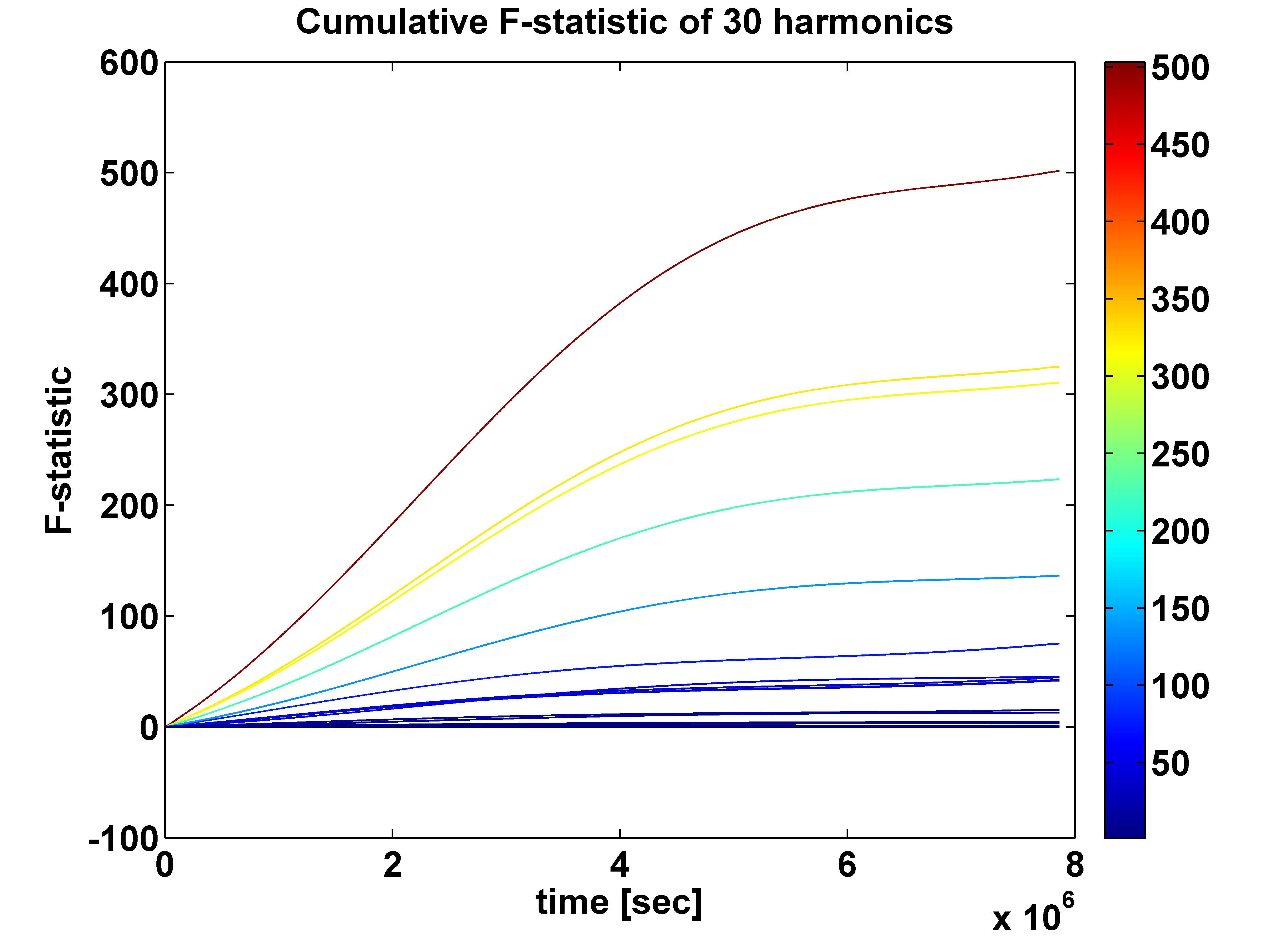
Figure 2: The cumulative F-statistic of 30 dominant harmonics with true parameters without noise. Since there is no noise, the F-statistic is not normalized.

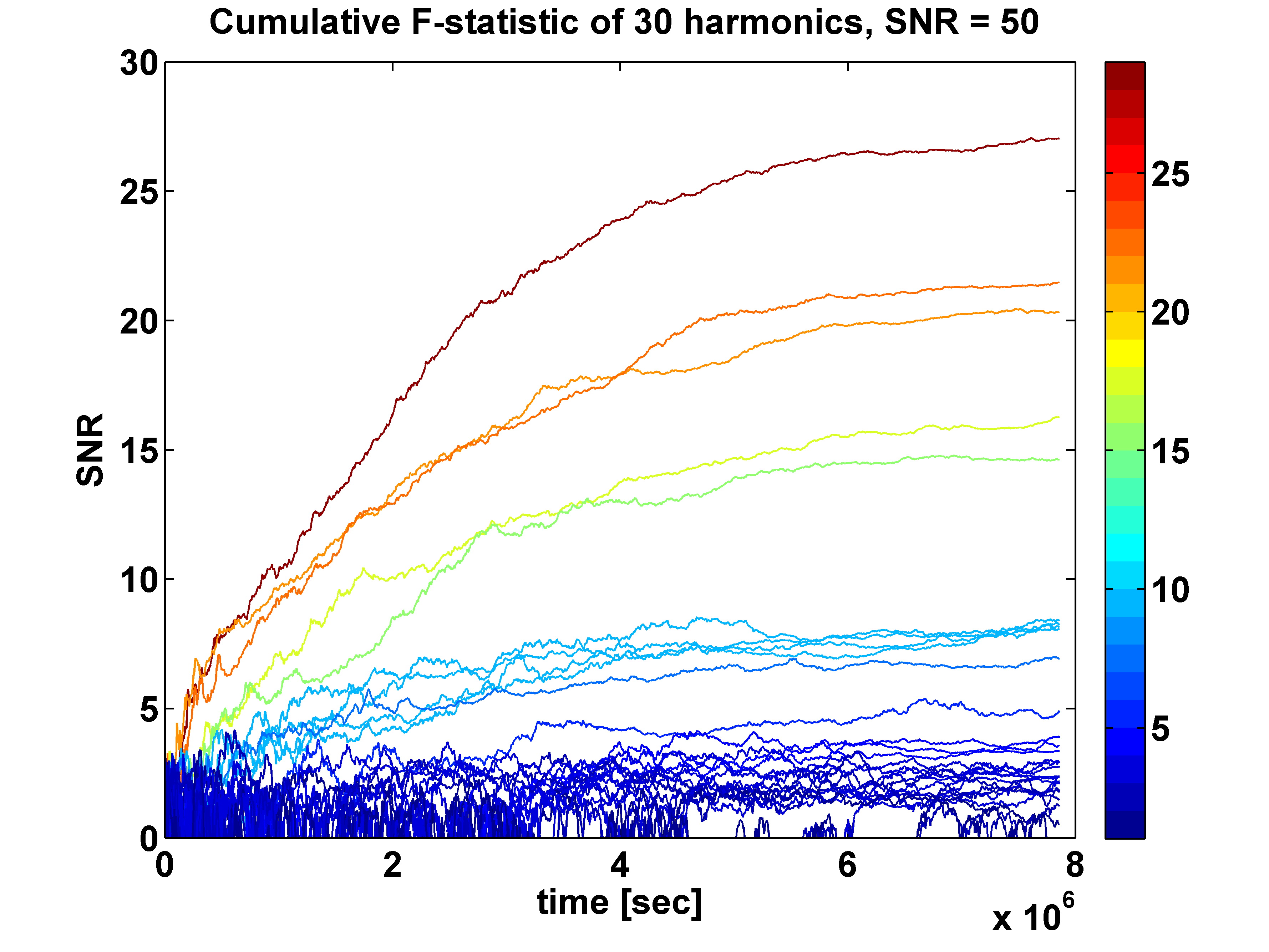
Figure 3: The cumulative F-statistic of 30 dominant harmonics with true parameters and detector noise. Note that the F-statistic is converted to $SNR$ in the figure. The strong harmonics are cumulating gradually with local spikes. The low-SNR harmonics behave similar to noise, hence made undetectable.

IV Search with the phenomenological waveform

In this section, we use the PW as described above together with the introduced detection statistic. We will use two 3 month worth simulated data sets: with and without noise. We use the same GW signal (based on NK model) in both cases. The total SNR of the source in the noisy case is 50. We have taken the following parameters for the EMRI : the mass of the MBH $M=10^{6}M_{\odot}$, the mass of the compact object (stellar mass BH) $m=10M_{\odot}$, the initial orbital eccentricity $e=0.4$, the semi-latus rectum $p=8M$, the inclination angle $\iota=\pi/9$, the spin of the MBH $a=0.9M$, the sky position of the source $(\theta^{S},\phi^{S})=(\pi/4,\pi/4)$, the polarization angle $\psi=0$. In our analysis we assume that the sky location is known. Our primary goal here is to recover the intrinsic parameters of the source.

The noiseless case is used to avoid any possible bias in the final result due to stochastic nature of the noise, and assess possible restrictions of our search technique and PW family. Next, we apply the same search method to the same GW signal buried in the noise, which would justify its effectiveness in practice.

Here, we describe the search for individual harmonics with Markov chain Monte Carlo (MCMC) method. For completeness and future references we give a brief introduction to MCMC. Like a standard Monte Carlo integration, MCMC is a random sampling method. It is nothing but Monte Carlo integration with a Markov chain. By properly constructing a Markov chain, MCMC can draw samples from the searching parameter space more efficiently. Among all the methodologies of constructing a Markov chain, the Metropolis-Hastings scheme would be the most general one. The main idea of Metropolis-Hastings algorithm is to cleverly construct a Markov chain that satisfy the detailed balance equation, so that the sampling distribution will converge to the likelihood surface we want to estimate. If the shape of the likelihood surface is known, the parameter set that corresponds to the maximum likelihood is automatically known. Thus, MCMC is also widely used as a stochastic optimization tool in GW data analysis (we refer the reader to a very nice overview and discussion on Bayesian methods in Littenberg:2009bm , see also references therein).

If the likelihood surface is multimodal(i.e. contains large number of separated local maxima) then simple version of the MCMC finds a maximum and does not move off it to explore larger parameter space. Many ways around this problem were suggested but we will not use any of them here (besides simulated annealing which we will discuss a later). As we will see, a simple Metropolis-Hastings algorithm is sufficient. The likelihood surface of an EMRI signal is very rich in “wall” and “needle” like structures, which make it very hard to find a global maximum. We are interested in detecting as many local maxima as possible. Therefore we run multiple independent chains and harvest the results after they converge to various maxima of the likelihood surface. If we are lucky, the global maximum could be among multiple maxima we have found.

To understand the Metropolis-Hastings algorithm, first consider a stochastic process denoted by $\{\bm{\theta}_{k}|k=0,1,2...\}$ which belongs to the parameter space $\mathcal{B}$ in $\mathbb{R}^{n}$. Here we defined $\bm{\theta}_{k}$ as a set of parameters at step $k$, which can also be viewed as a point in the parameter space $\mathcal{B}$. If there exists a transition probability $P(\bm{\theta}_{k+1}|\bm{\theta}_{k})$ depending only on the current point $\bm{\theta}_{k}$ for the stochastic process to be in state $\bm{\theta}_{k+1}$, we call this stochastic process $\{\bm{\theta}_{k}|k=0,1,2...\}$ a Markov chain with a transition probability $P(\bm{\theta}_{k+1}|\bm{\theta}_{k})$. In a Bayesian viewpoint, we can take this transition probability as conditional probability and immediately see that

$$\int_{\mathcal{B}}P(\bm{\theta}_{k+1}|\bm{\theta}_{k})d\bm{\theta}_{k+1}=1\;.$$ (28)

A Markov chain satisfying the detailed balance equation

$$\Lambda(\bm{\theta}_{k})P(\bm{\theta}_{k+1}|\bm{\theta}_{k})=\Lambda(\bm{\theta}_{k+1})P(\bm{\theta}_{k}|\bm{\theta}_{k+1})$$ (29)

will (up to some relatively weak conditions) be equivalent to the samples from the distribution $\Lambda(\bm{\theta})$ after a certain initial period (often called burn-in stage). We can easily estimate the distribution $\Lambda(\bm{\theta})$ with the Markov chain samples and hence the most probable parameter set $\hat{\bm{\theta}}$ for given observed data $\bf{s}$, where

$$\Lambda(\hat{\bm{\theta}}|\bf{s})=\max_{\bm{\theta}}\Lambda(\bm{\theta}|\bf{s})$$ (30)

is usually called the maximum likelihood estimator.
By virtue of Metropolis-Hastings algorithm, we can construct a Markov chain that satisfies the detailed balance equation and make use of the corresponding property to estimate our template parameters $\bm{\theta}$. To do this, we randomly choose a parameter set $\bm{\theta}_{0}$ in the parameter space as the starting point. Then one can pick a proposal distribution $q(\bm{\theta}_{k+1}|\bm{\theta}_{k})$ (as long as there is no forbidden region in the prescribed parameter space to the point $\bm{\theta}_{k+1}$) and sample a candidate point $\bm{\theta}_{k+1}$ from this distribution. Then we calculate the acceptance probability defined by the following formula

$$\alpha(\bm{\theta}_{k},\bm{\theta}_{k+1})=\min\left(1,\frac{\Lambda(\bm{\theta}_{k+1})q(\bm{\theta}_{k}|\bm{\theta}_{k+1})}{\Lambda(\bm{\theta}_{k})q(\bm{\theta}_{k+1}|\bm{\theta}_{k})}\right)\;.$$ (31)

By accepting the point $\bm{\theta}_{k+1}$ according to the above probability, we have, in fact, succeeded to construct a transition probability,

$$P(\bm{\theta}_{k+1}|\bm{\theta}_{k})=q(\bm{\theta}_{k+1}|\bm{\theta}_{k})\alpha(\bm{\theta}_{k},\bm{\theta}_{k+1})\;.$$ (32)

It is easy to see that the Markov chain generated by the above transition probability satisfies the detailed balance equation:

$$\Lambda(\bm{\theta}_{k})P(\bm{\theta}_{k+1}|\bm{\theta}_{k}) = \min\left(\Lambda(\bm{\theta}_{k})q(\bm{\theta}_{k+1}|\bm{\theta}_{k}),\Lambda(\bm{\theta}_{k+1})q(\bm{\theta}_{k}|\bm{\theta}_{k+1})\right)$$ (33)

$$= \min\left(\Lambda(\bm{\theta}_{k+1})q(\bm{\theta}_{k}|\bm{\theta}_{k+1}),\Lambda(\bm{\theta}_{k})q(\bm{\theta}_{k+1}|\bm{\theta}_{k})\right)$$

$$= \Lambda(\bm{\theta}_{k+1})P(\bm{\theta}_{k}|\bm{\theta}_{k+1}).$$

Thus, such a Markov chain will eventually serve as a succession of samples from $\Lambda(\bm{\theta})$. The best performance is achieved if the proposal probability $q(\bm{\theta}_{k+1}|\bm{\theta}_{k})$ resembles the target distribution $\Lambda(\bm{\theta})$ over the entire parameter space. Without prior knowledge about the kind of probability distribution around the true parameter location, it is natural to choose it as a multivariate normal distribution centered at the present point $\bm{\theta}_{k}$ with covariance matrix $\mathcal{C}$,

$$q(\bm{\theta}_{k+1}|\bm{\theta}_{k})=\frac{1}{\sqrt{(2\pi)^{N}\mathrm{det}[\mathcal{C}]}}\exp{\left[-\frac{1}{2}(\bm{\theta}_{k+1}-\bm{\theta}_{k})^{\textsf{T}}\mathcal{C}^{-1}(\bm{\theta}_{k+1}-\bm{\theta}_{k})\right]}\;,$$ (34)

where $N$ denotes the dimension of the parameter space and $\mathrm{det}[\mathcal{C}]$ the determinant of the covariance matrix $\mathcal{C}$. The likelihood surface has usually multimodal (multiple local maxima) structure, and, therefore, a single multivariate normal distribution cannot describe the probability density over the entire template space but only a very small region around the local maximum. Since the probability distribution at the local maximum is usually very sharp, a Markov chain easily gets trapped there for many steps. To avoid insignificant maxima we use the so-called annealing scheme, originating from simulated annealing. We adopt two types of annealing techniques: (i). we introduce a temperature $\mathcal{T}_{1}$ to the acceptance rate $\alpha$ [equation (31)] so as to have a larger possibility to accept the proposal point in the beginning. By combining equations (17), (24), (31), (34), the acceptance probability is now written as

$$\alpha(\bm{\theta}_{k},\bm{\theta}_{k+1})=\min\left(1,e^{[F(\bm{\theta}_{k+1})-F(\bm{\theta}_{k})]/\mathcal{T}_{1}}\right)\;.$$ (35)

where the temperature $\mathcal{T}_{1}=\mathcal{T}_{1}(k)$ is a function of the step index $k$, it starts from some relatively large number and gradually decays to unity. (ii). We introduce a second temperature $\mathcal{T}_{2}$ to the proposal distribution $q(\bm{\theta}_{k+1}|\bm{\theta}_{k})$. The covariance matrix $\mathcal{C}$ is replaced by $\mathcal{C}\times\mathcal{T}_{2}$. Same as $\mathcal{T}_{1}$, $\mathcal{T}_{2}$ is also a function of the step index $k$, decaying gradually to unity. Hence, the chain take large steps in the beginning and explores large volume in the parameter space. Explicitly, we choose $\mathcal{T}_{1}$ and $\mathcal{T}_{2}$ both as a linear function of $k$ with negative slope.
Let us summarize the algorithm:

1. $k=0$. Choose a random parameter set $\bm{\theta}_{0}$ as the starting point and calculate the F-statistic $F(\bm{\theta}_{0})$.

2. $k\rightarrow k+1$. Calculate the temperature $\mathcal{T}_{1}(k),\mathcal{T}_{2}(k)$.

3. Generate the next candidate parameter set $\bm{\theta}_{c}$ from the proposal distribution with modified covariance $\mathcal{C}\times\mathcal{T}_{2}$.

4. Calculate the F-statistic of the new parameter set $F(\bm{\theta}_{c})$.

5. Calculate the acceptance probability $\alpha(\bm{\theta}_{k},\bm{\theta}_{c})=\min\left(1,e^{[F(\bm{\theta}_{c})-F(\bm{\theta}_{k})]/\mathcal{T}_{1}}\right)$.

6. Draw a random number $u$ from unity distribution $\mathcal{U}(0,1)$. If $u<\alpha$, accept the candidate parameter set $\bm{\theta}_{k+1}=\bm{\theta}_{c}$, else, stay at the current point $\bm{\theta}_{k+1}=\bm{\theta}_{k}$.

In the search we have used a diagonal form of the covariance matrix in the gaussian proposal distribution (34), with the following elements: $\mathcal{C}=[\mathrm{diag}(10^{-4},\,10^{-12},\,10^{-20},\,10^{-28})]^{2}$ corresponding to the parameter set $\{f,\dot{f},\ddot{f},\dddot{f}\}$. And $\mathcal{T}_{2}$ used to scale the covariance matrix decays linearly with the number of members in the chain from 1 to $5\times 10^{-4}$. We have found that the use of the actual Fisher information matrix as $\mathcal{C}$ did not improve significantly the search results. We run about 50 chains on both noiseless data and noisy data. All the parameter sets that generate an SNR larger than a certain threshold (we have used $SNR>4.5$) are recorded. Notice that there are possibly many such qualified parameter sets in a single chain. Thus, we have hundreds to thousands of qualified parameter sets or local maxima. These local maxima contain information about the signal. We will analyze these local maxima in the next section.

V Analysis of the search results and mapping to the physical parameters

In this section we will explain how we use the results of MCMC search described in the previous section and reconstruct harmonics of the GW signal. Furthermore, we use the model of EMRI (NK) to estimate the physical parameters of the system.

V.1 Clustering algorithms

In this subsection we extract information from the local maxima detected by MCMC search. We first focus on the noiseless data to explain the algorithm, then modify it a bit and apply it to the noisy data. Since this work is the first of a series of papers, the main task here is to establish the framework and justify the method. Hence, as mentioned above, we have assumed that the sky position of the source is known and concentrate on the intrinsic parameters only. This will save us some time, yet maintain all the main features of the problem. As a result, each local maximum is characterized only by the frequency and its derivatives $(f,\dot{f},\ddot{f},\dddot{f})$.

Let us look at one example to understand how we extract the information about the source from the detected local maxima. We take a particular solution of MCMC search and for each harmonic of PW we can compute cumulative F-statistic according to the prescription given in Section III.3. We concentrate only on those harmonics which give significant contribution to the total F-statistic. If the harmonics of PW match perfectly the harmonics of a signal we should observe something similar to Fig. 3, however it is rare when we detect a full harmonic (only sometimes for the strongest). More frequently, we detect a part of a harmonic (frequency and derivatives close to true but not exact) or even several harmonics at different instances of time as shown in Fig. 4. The black and green curves are two strong harmonics of a signal (black being stronger), and the blue is a harmonic of PW. In the pink regions, our template matches for a short period of time the frequency of a signal (two distinct harmonics at two instances). The corresponding cumulative F-statistic is shown in Fig. 5. There are two positive jumps in the accumulation of the F-statistic which correspond to two instances of intersection. Therefore, we can conclude that the positive slope in the cumulative F-statistic (if it happens over a significant duration) corresponds to the part of the frequency and time where a harmonic of PW matches (at least partially) some harmonics of a signal. We collect such events of matching and display them on the time-frequency plane, resembling the mosaic of a true signal.

The violent oscillation in Fig. 5 is one of the three types of oscillations on the cumulative F-statistic curve mentioned in the previous section. In fact, it is the beat note between the true harmonics and the local maximum. Observe that the beat notes happen at relatively higher frequency, while the increasing slopes (where the local maximum matches the frequencies of the true harmonics) have relative low frequency. Thus, we design a third-order Butterworth low pass filter to get rid of the beat notes. After the low-pass filter, the cumulative F-statistic has only few extrema, as shown in Fig. 6. After clearing up the cumulative F-statistic, we apply two criteria for identifying a significant F-statistic accumulation: (i) the slope must be larger than certain threshold; (ii) the accumulation time must be over longer than certain period. As it is seen by eye tuning those two parameters should be sufficient to get the right parts of cumulative F-statistic. In our search we have made the following choice for those parameters. In the case of noiseless data, we require the slope to be larger than one-tenth of the largest slope of the cumulative F-statistic of that trial harmonic, and the cumulative time (over which we observe steep positive slope) to be longer than three days.

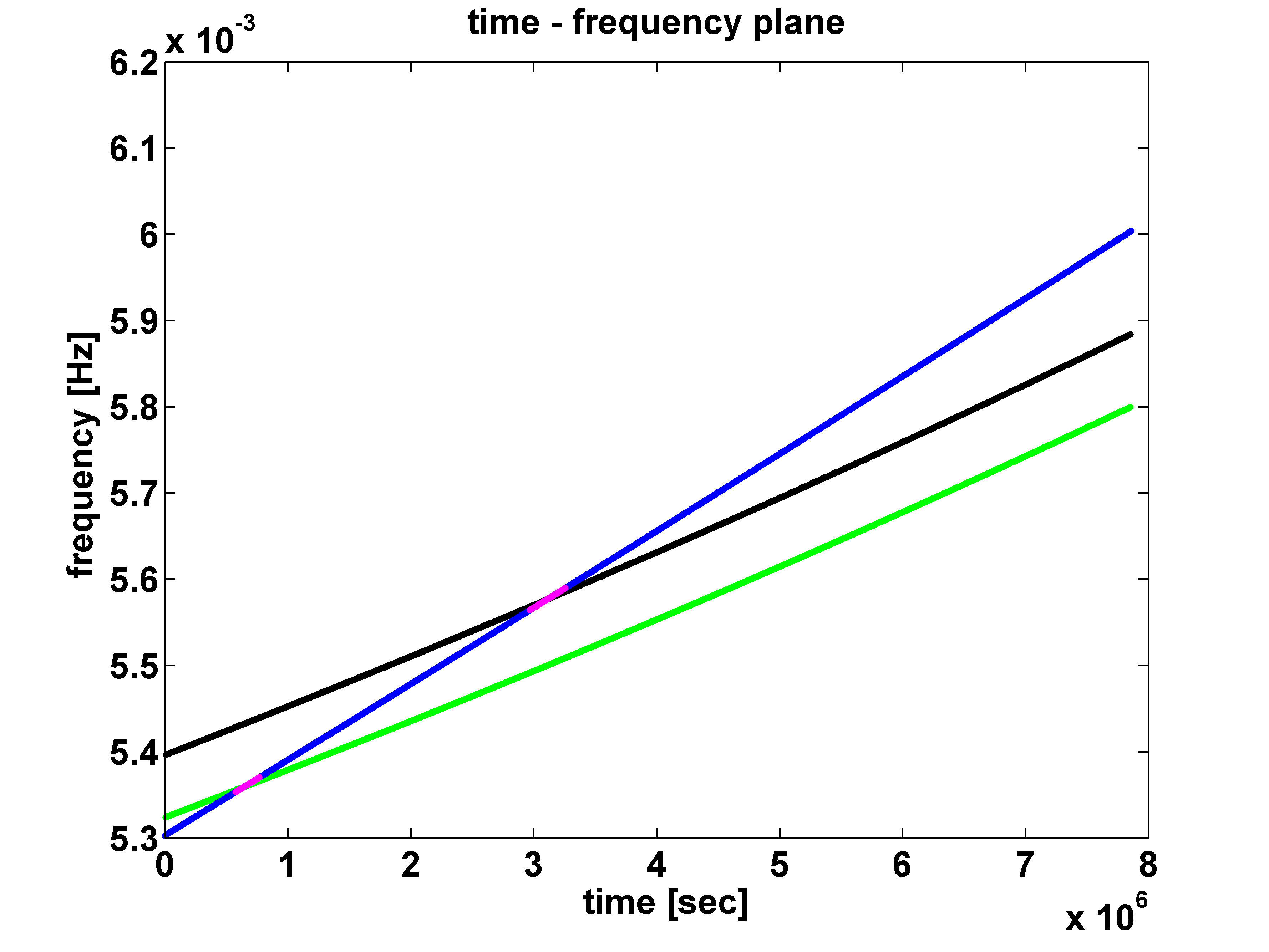
Figure 4: Time-frequency plot of harmonics. The black and green tracks are two strong harmonics of the EMRI signal (black being stronger). The blue track corresponds to a harmonic of PW that accumulates a significant F-statistic. It intersects the true harmonics at the pink segments, those correspond to times of increase of F-statistic, see Fig. 5, 6.

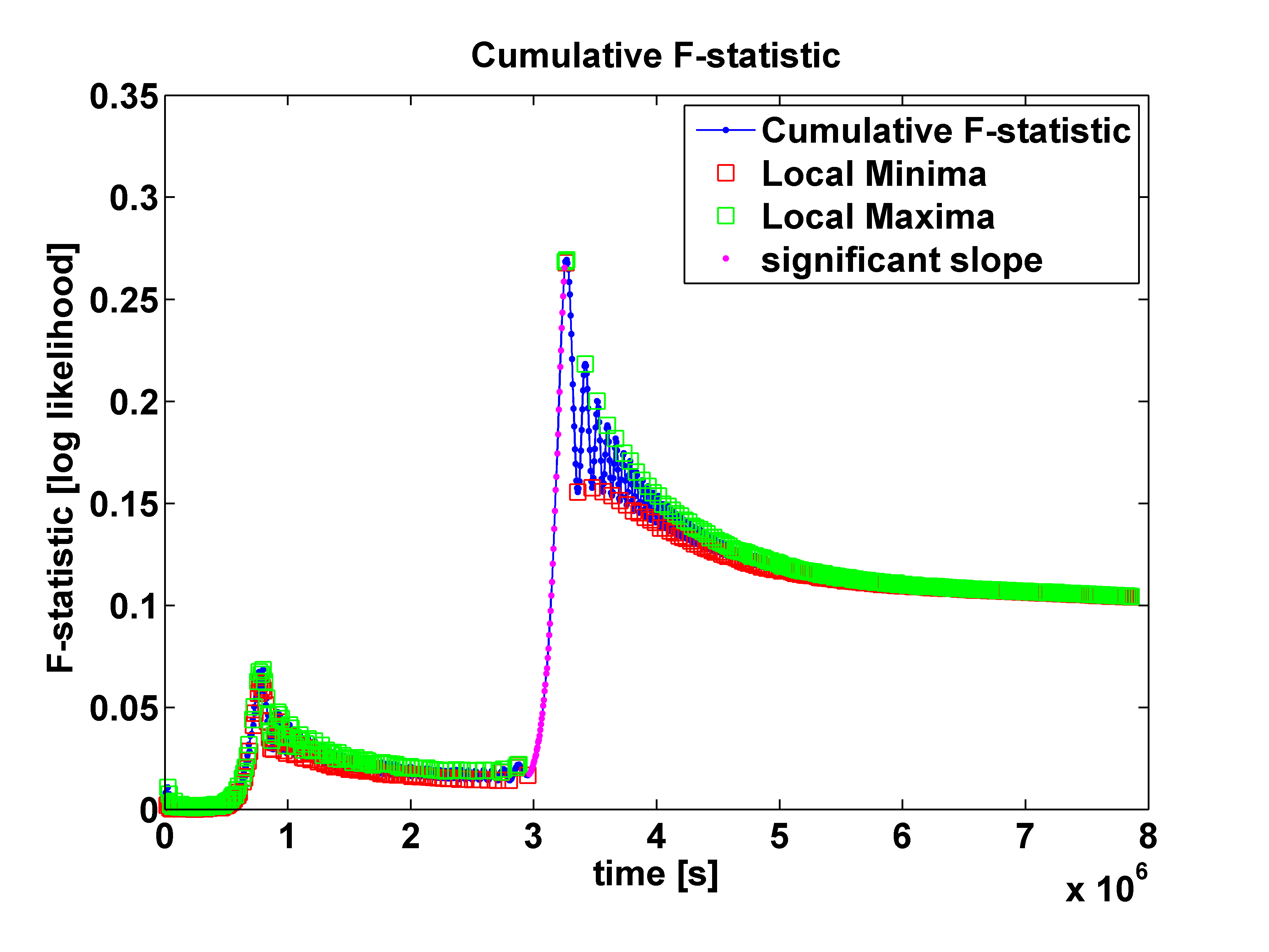
Figure 5: Unfiltered cumulative F-statistic corresponding to the PW harmonic and data given in Fig. 4. The F-statistic labeled on the vertical axis has only relative meaning, since we work with the noiseless data. The green and red squares mark the extremes of the curve, thus distinguishing between the increasing and the decreasing slopes. The large number of the extremes is due to the beating between the true harmonics and the trial harmonic.

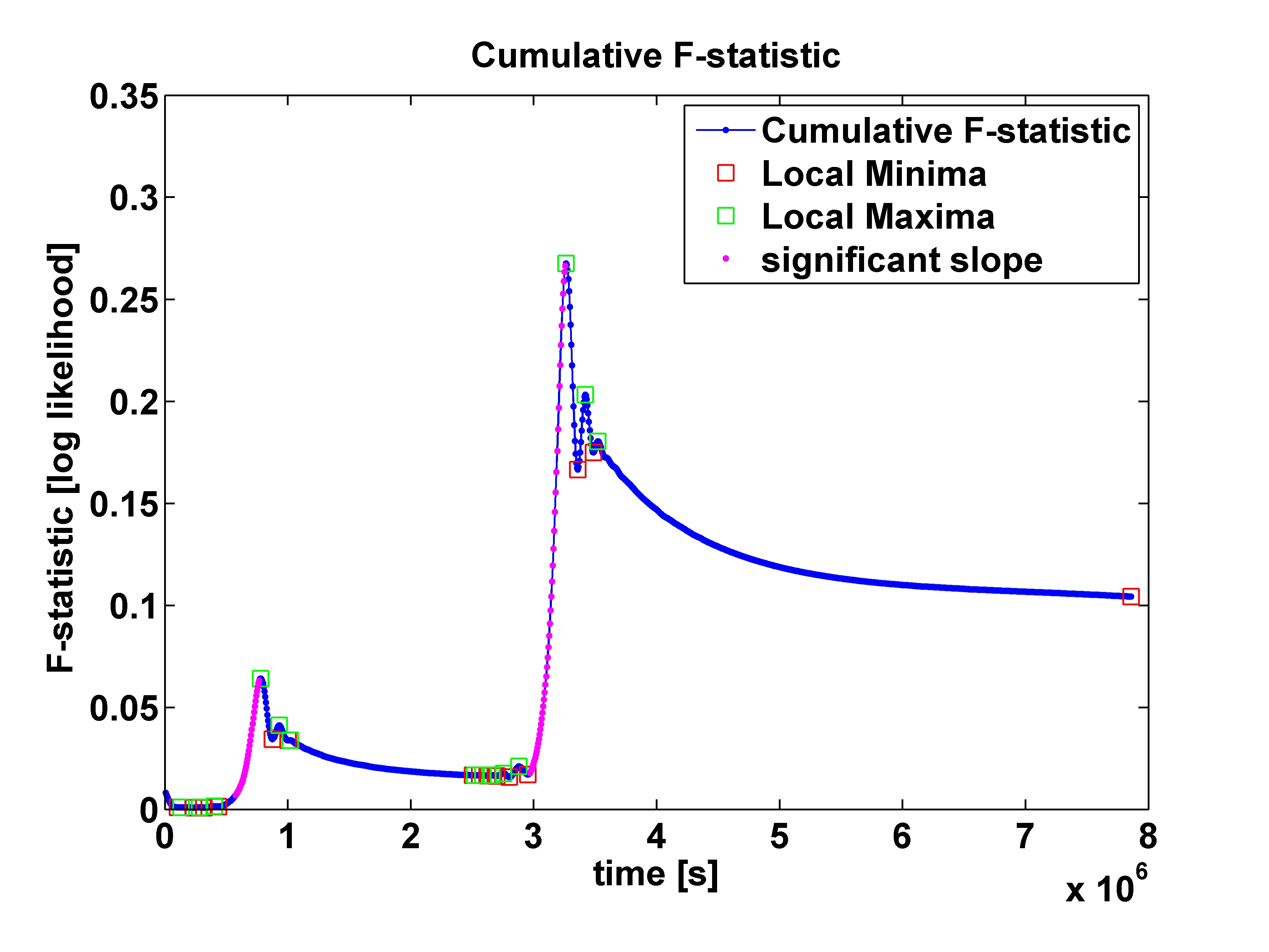
Figure 6: Filtered cumulative F-statistic corresponding to the situation depicted in Fig. 4. It is similar to Fig. 5, but after applying the low pass filter to remove the beatings (high frequency oscillations).

We plot all recovered patches on the time-frequency plane in Fig. 7, where we can identify by eye 13 strong harmonics. Although the weaker harmonics are lost, the strong ones retain enough information about the EMRI system evolution, hence allowing us to recover the physical parameters we are interested in. Zooming at a specific harmonic in time and frequency, one will see that there are many patches from different results and at each instant we observe a finite spread in the frequencies for a given harmonic. This is due to various solutions from MCMC search matched a given harmonic of a signal with different precision. However, we expect that the distribution of found frequencies at each instant of time will be centered at the true frequency of the signal’s harmonic. As an example, we show distribution of found frequencies at a particular instance of time for two harmonics in Fig. 8. In that plot we show the histogram of detected frequencies at that time in blue and Gaussian fit as smooth green curves. This is to be compared with frequencies of two harmonics of a signal at the same time in red. As mentioned above, different solutions of MCMC search vary in precision of matching the signal at different instances, and we can use accumulation time as a measure of goodness of match of a signal by a given solution. The relative accumulation time of different solutions are shown as pink points in Fig. 8. First, one can see that Gaussian fit lies on the top of the true frequency, and second, that the distribution of pink points is similar to the blue histogram, so either can be taken to characterize the found harmonics of a signal. Similarly, we can do at each instance of time for all found tracks in the time-frequency plane. For the noiseless search we picked uniformly 10 instances and made a Gaussian fit around each harmonic. We identify the mean of the Gaussian fit as the most likely frequency of a signal’s harmonics at that instance and we identify the spread (standard deviation) of a distribution as an error in our evaluation of a frequency. The result of this clustering is given in Fig. 9.

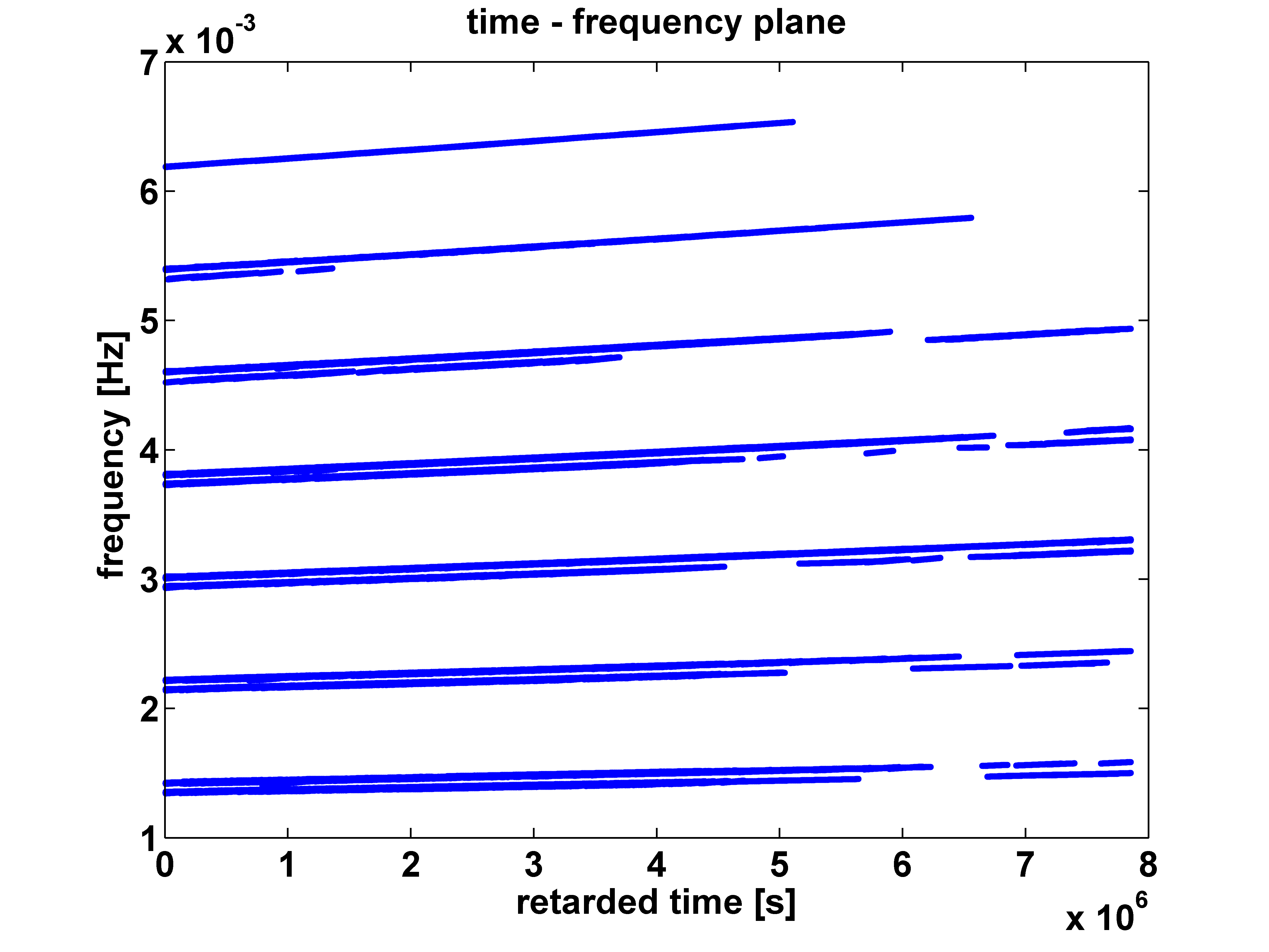
Figure 7: Time-frequency plot of all patches corresponding to strong accumulation of F-statistic. We can identify parts of frequency tracks of 13 EMRI harmonics. Each track in this plot has a finite width coming from different solutions of MCMC search which have different precision of matching the signal.

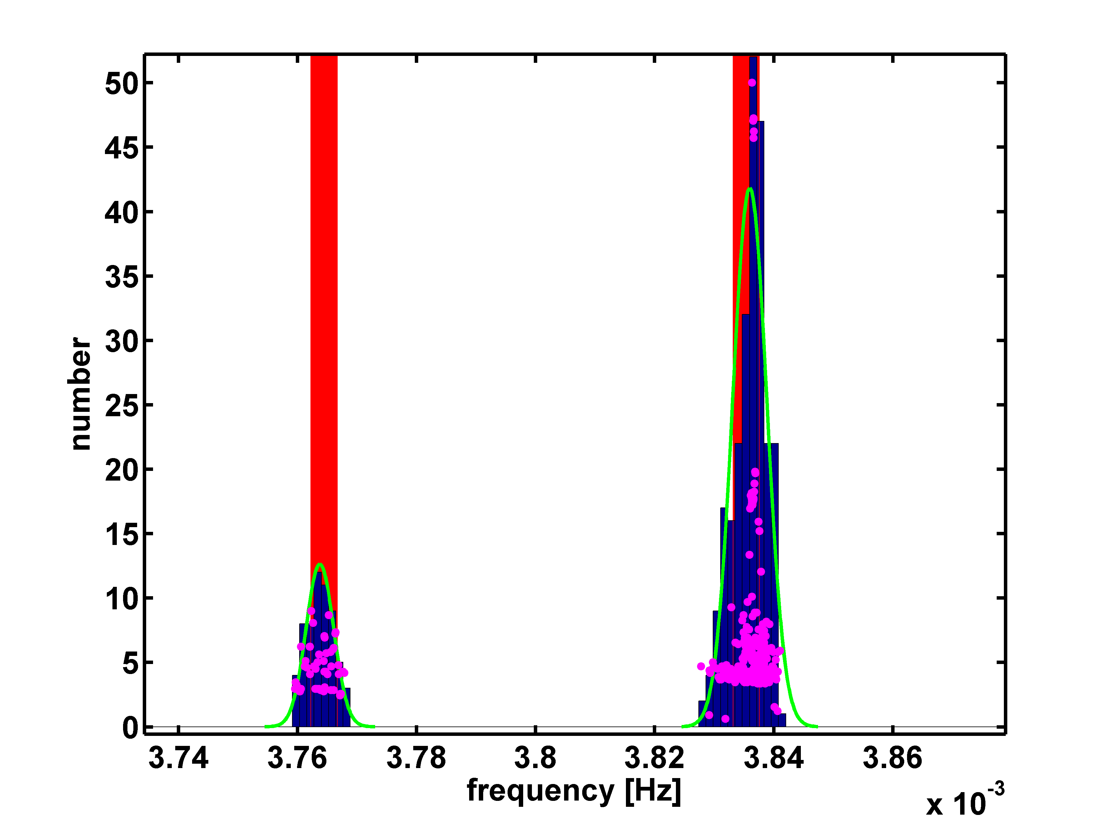
Figure 8: Zoom at two harmonics at a specific instance of time. The red stems denote the frequencies of the true harmonics of a signal, while the blue histogram shows the detected frequencies at this instant. The green curves display the Gaussian fit to the frequency data with re-scaled amplitudes. The vertical axis of pink points indicates the relative time over which we have observed strong accumulation of F-statistic for each solution.

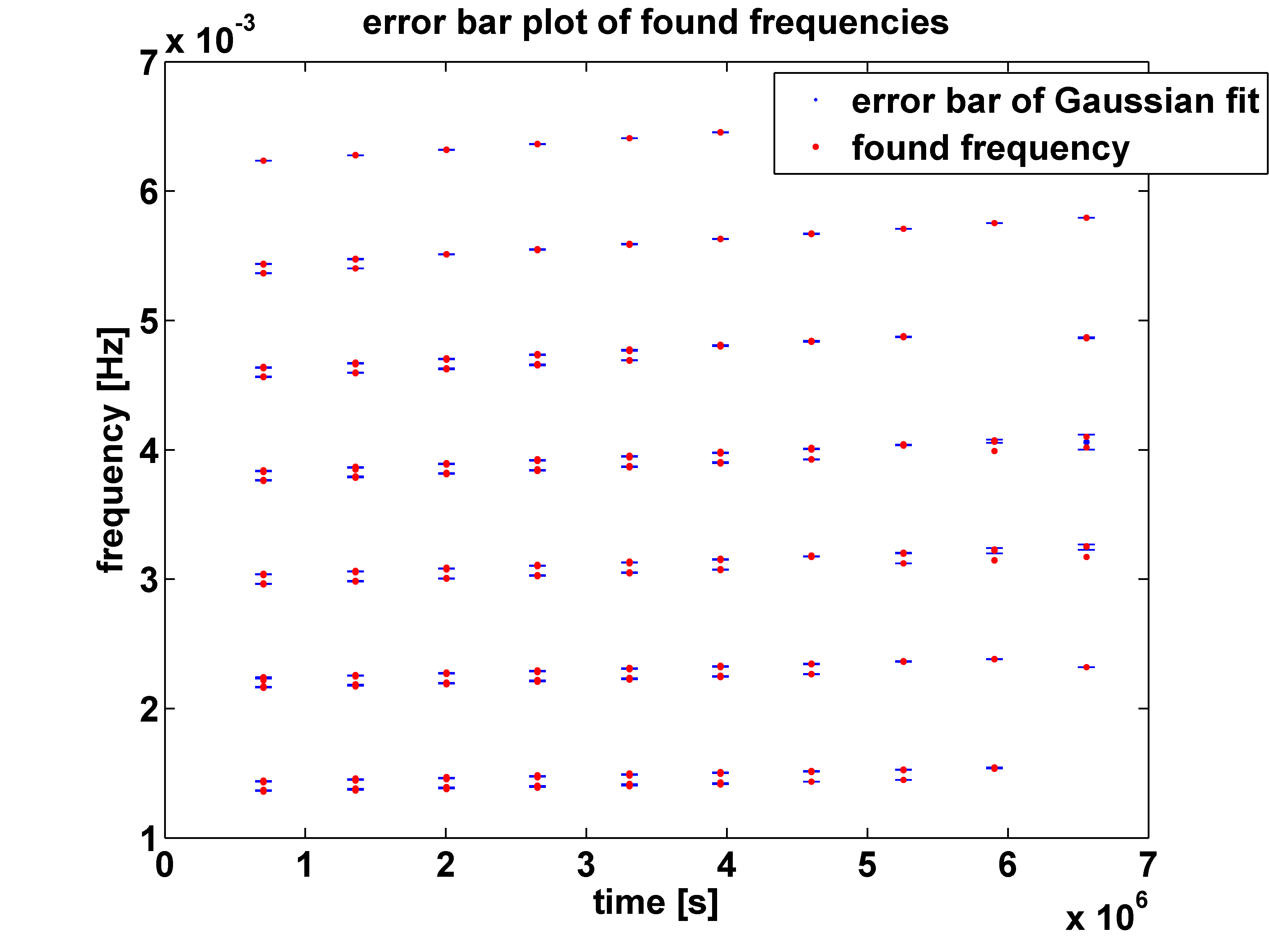
Figure 9: Gaussian fit to the detected frequencies at ten instants. The red points represent the mean of a Gaussian fit as shown in Fig. 8 for each harmonic at ten instants . The blue error bars show the $1\sigma$ uncertainties of the Gaussian fits. Note the tiny error bars are along the frequency dimension which indicates that the MCMC search localizes quite well frequencies of the EMRI’s harmonics.

In the case of data with the detector noise, the basics and the strategy are roughly the same as in the noiseless case with minor modifications. In the beginning, we record the local maxima with SNR greater than $4.5$. Next, we select the significant increasing slopes of the cumulative F-statistic with three requirements: (i) the maximum F-statistic along the cumulative F-statistic curve is larger than $50$, (ii) the minimum slope of the significant increasing segment is larger than $4\times 10^{-6}s^{-1}$, (iii). the monotonic increasing duration is longer than about a week. Those conditions are more stringent than for the noiseless case and eliminated several found weak harmonics of EMRI signal. However, at the same time they significantly reduce the false events (and that is what we want). From this selection, we identify 5 strong harmonics in the noisy case. After that the procedure is similar to the noiseless case.

V.2 Search for physical parameters

Now we are in a position to recover the physical parameters of the binary system. First, we need to adopt the model for the orbital evolution, and here we used the same model as used in the simulation of the data sets. In the noiseless case the only reason for the deviation of recovered parameters from the true values is due to inaccurate identification of the tracks in the time-frequency plane or due to ambiguity in solving the inverse problem (mapping harmonic tracks onto the physical parameters, $m/M,a,e,\iota,p/M$). We have performed the search on the time-frequency plane similar in spirit to Gair:2008ec . We have used weighted chi-square test

$$\chi^{2}=\sum\min_{f_{lmn}}\left(\frac{f_{lmn}-f_{\mathrm{mean}}}{\sigma_{f}}\right)^{2}$$

between signal tracks (for different parameters) and recovered tracks (Fig. 9). We have used particle swarm optimization (PSO) and genetic algorithm (GA) as two independent search methods to test the robustness of our result. We start with describing the PSO method, and then give brief overview of GA.

Particle swarm optimization (PSO) is a stochastic optimization method introduced by Kennedy and Eberhardt in 1995 Kennedy95 . In gravitational wave data analysis, PSO was first applied to a binary inspiral signal Wang:2010jma . In this section, we briefly describe the algorithm, while further details can be found in the references Kennedy95 ; Wang:2010jma .
The goal of PSO is to find the global minimum/maximum (here we minimize the chi-square test) of a parameterized functional $\kappa(\bm{\theta})$ and the corresponding parameter set $\bm{\theta}_{*}$, where $\bm{\theta}$ stands for an arbitrary parameter set in $\mathbb{R}^{n}$. The idea is to evaluate $\kappa(\bm{\theta}_{i})$ simultaneously at different parameter sets $\bm{\theta}_{i},\,i=1,2,...$, treating them as particles in the parameter space, and evolve them according to certain dynamics until the stable solution is reached. Let us denote the $i$-th particle out of a swarm of $N_{p}$ particles during $k$-th iteration in the search by $\bm{\theta}_{i}[k]$. Its position in the parameter space in the next iteration is determined by its velocity in the current iteration $\bm{v}_{i}[k]$,

$$\bm{\theta}_{i}[k+1]=\bm{\theta}_{i}[k]+\bm{v}_{i}[k].$$ (36)

Usually, the particles start with randomly chosen positions $\bm{\theta}_{i}[1]$ and velocities $\bm{v}_{i}[1]$. Up to $k$-th iteration, we denote the $i$-th particle’s best location by $\bm{\theta}^{p}_{i}[k]$, in the sense that

$$\kappa(\bm{\theta}^{p}_{i}[k])=\min_{j\leq k}\kappa(\bm{\theta}_{i}[j]).$$ (37)

The global best location $\bm{\theta}^{g}_{i}[k]$ up to the $k$-th iteration is defined by

$$\kappa(\bm{\theta}^{g}[k])=\min_{i}\kappa(\bm{\theta}^{p}_{i}[k]).$$ (38)

Note that particle best locations and the global best location are the best parameters respectively found by the individual particles and the whole swarm in the entirely history of the search up to the $k$-th iteration. They are updated only when a better parameter set is found. These best locations contain a lot of information about the functional $\kappa(\bm{\theta})$, so they are used to guide the particle’s motion in the future. Explicitly, the velocities are updated with the following equation

$$\bm{v}_{i}[k+1]=w\bm{v}_{i}[k]+c_{1}\chi_{1}(\bm{\theta}^{p}_{i}[k]-\bm{\theta}_{i}[k])+$$

$$c_{2}\chi_{2}(\bm{\theta}^{g}[k]-\bm{\theta}_{i}[k]),$$ (39)

where $w$ is called the inertia weight, $c_{1},\,c_{2}$ are called the acceleration constants (we take them to be the same as in Wang:2010jma ) and $\chi_{1},\,\chi_{2}$ are random numbers drawn from $\mathcal{U}(0,1)$. We run PSO search several times until the return result is confirmed by several searches.

The second search method is called Genetic Algorithm (GA) and there we evolve a number of parameter sets (points in the parameter space $\mathbb{R}^{n}$). Each parameter set $\bm{\theta}_{i}$ is called an organism, individual parameters are called the genes of this organism and the set of organism at $k$-th search iteration step is called $k$-th generation. We evolve generations according to the prescribed rules called “parents selection”, “breading” and “mutation”. The main idea of this optimization technique is to evolve colony of organisms toward the better fitness (which could be likelihood ratio or, in our case, chi-square value) like in Darwin’s theory of natural selection. The strong organisms (with better fitness) participate more often in breading and therefore drag the colony toward the better values (lower) of chi-square. Mutation brings element of randomness in the search and occasional “positive” mutations help to avoid trapping around local minimum. For use of GA in GW data analysis we refer to Crowder:2006wh ; Petiteau:2010zu and references therein.

Let us give few more details specific to the implementation used in here. We use $\chi^{2}$ value as a measure of fitness for each organism (smaller value is better). In each generation we use the roulette method with the selection probability proportional to the fitness of each organism. For breeding we have used the one random point crossover rule. The probability mutation rate is monotonically decreasing function of the generation number: we have started with high probability of mutation to explore a large part of the parameter space and decrease it gradually as organisms converge to a particular part of the parameter space. We have used “children” and “parents” sorted in the fitness to make a new generation: we use 50% of the best organisms. We automatically achieve the “elitism” in a way that the best $\chi^{2}$ value is never increasing from one generation to the next.

We use the multi-step method to accelerate the search. In each step we evolve the colony for 500 generations as described above, but each new step uses the last generation of the previous step as the initial state. We have started evolution in the first step with completely random distribution of the organisms. The evolution of the colony at each step finishes with a very small mutation probability and with organisms confined to a quite small volume of the parameter space. The consequent search steps ensure that the found solution is a robust solution with respect to increase of the mutation probability which disperses organisms forcing them to explore the parameter space for presence of a solution with better fitness. This helps to avoid being trapped in the local minima. The termination condition is the stability of the best solution over several steps of the search.

We have applied both those methods to fit the found tracks on the time frequency plane with the harmonics of EMRI signal. The search is done in 5 dimensional parameter space with quite broad priors on $(e,p/M,\iota,a,\mu=m/M)$, those are the eccentricity, the semi-latus rectum, the orbital inclination angle at the moment of beginning of observation, the spin of the MBH, and, the mass ratio between the stellar BH and the MBH. The total mass is not present here, we have kept it fixed to $M=10^{6}M_{\odot}$. For a given set of parameters, our search algorithm computes three fundamental orbital frequencies as functions of time, then a weighted chi-square goodness of fit test is preformed on harmonics of the signal. We use the means and standard deviations from the Gaussian fit as found point and its error in the time-frequency plane. The best fit corresponds to the lowest value of $\chi^{2}$. We have used harmonics of the signal, which are expected to be strong over the large part of the parameter space, and have found this “harmonic table” by intensive monte carlo with NK models generated in the frequency domain. The index table has been truncated by choosing harmonics contributing (in total) 90% of the overlap with a total signal .

The recovered parameters are given in the table 1.

Table 1: Recovered parameters of EMRi against actual parameters used in simulated data sets.

description	$e(t_{0})$	$p(t_{0})$	$\iota(t_{0})$	a	$\mu$
True parameters	0.4	8.0	0.349	0.9	$10^{-5}$
Recovered parameters (with noise)	0.395	8.029	0.342	0.891	$9.79\times 10^{-6}$
Recovered parameters (no noise)	0.402	7.991	0.360	0.901	$1.002\times 10^{-5}$

VI Summary

In this paper we have introduced the phenomenological family of waveforms (PW) for detecting EMRI signals in the data from the LISA-like observatory. The template is constructed out of independent (over the time interval we have applied our analysis) harmonics of slowly evolving three orbital frequencies. We have neglected the amplitude evolution and presented the phase as a Taylor series up to the third derivative of frequency. Our analysis was restricted to the case of monotonically increasing frequencies. This condition will break only close to the plunge. The number of harmonics and range of indices were taken from the analysis of dominant harmonics of our model signal, though we have found at the end that the search only weakly depends on the number of used harmonics (only through the accumulated total SNR, which should be sufficient to claim detection).

Constructed phenomenological templates allows us to search for EMRI signals in a model independent way. This way we avoid complexity of accurate modeling the orbital evolution and gravitational waveform during the search. In addition PW cover also all possible small deviations of the background spacetime from the Kerr solution which would influence the signal’s phase and could lead even to loss of the signal if the template assumes pure Kerr background geometry.

We have used MCMC based search to find a large number of local maxima of the likelihood surface. We were not that lucky to find the global maximum. We have analyzed the found solutions by means of cumulative F-statistic over the time and identified the patches of the signal which were match by templates. As a result, we have constructed a time-frequency map of (parts of) the signal’s harmonics. Each track could be characterized by the best guess and the error bar at each instance of time (by fitting Gaussian profile to found frequencies around at that time each track). The next step is to assume a model for the binary orbital evolution, and check if the found time-frequency picture corresponds to the strongest harmonics of a signal. In other words, we want to find the physical parameters of the binary system which strong GW harmonics could leave the found imprint. We do that by conducting a search using particle swarm optimization techniques and, independently, genetic algorithm. We have used weighted chi-square goodness of fit test to choose the best matching harmonics of the signal. We have assumed the same model as was used in the simulated data, and the recovered parameters are within 2% of the true values.

We want to make few final remarks. (i) The found time-frequency tracks of the GW signal from EMRI did not assume any particular model. The mapping of these tracks to the physical parameters could be done in post processing using several models. We have chosen on purpose rather short (3 month) duration of the data. The search procedure could be repeated for each three months and then one can check consistency of a given model or further improve accuracy in the recovered parameters (if our model gives consistent parameters of the system across different data segments). This could be a powerful method to search deviations from “Kerness”. (ii) In the mapping of the time-frequency tracks to the physical parameters of the binary, we have only weakly used information about the strength of each track/harmonic. We have found that the information stored in the frequency evolution is sufficient to recover parameters of EMRI. However, additional information about the strength of the recovered harmonics and harmonics of the modeled GW signal could give us additional confidence in the result and/or distinguish between several solution, if ambiguity happens. (iii) Mapping from the found time-frequency tracks onto the physical parameters might turn out to be the most computationally intensive task. However, one might use the information about the strength and a number of found harmonics to restrict a volume of the searched parameter space. In addition, to perform mapping we require mainly the computation of the orbital evolution, not the full waveform. However, it is then important to know which harmonics are the strongest for a given parameter set. (iv) In the future work we intend to include the sky location and the MBH mass into the search and investigate the possibility to differentiate between different models of EMRIs based on the results of MCMC search with PW (as discussed in (i)).

VII Acknowledgement

The authors would like to thank S. Drasco and J. Gair for useful discussions. The work of S. B. and Y. W. was partially supported by DFG Grant No. SFB/TR 7 Gravitational Wave Astronomy and DLR (Deutsches Zentrum fur Luft- und Raumfahrt). Y. W. also would like to thank the German Research Foundation for funding the Cluster of Excellence QUEST-Center for Quantum Engineering and Space-Time Research. Y. S. was supported by MPG within the IMPRS program.

References

- (1) L. Barack and C. Cutler, Phys. Rev. D, 69, 082005 (2004), arXiv:gr-qc/0310125
- (2) L. Barack and C. Cutler, Phys. Rev. D, 75, 042003 (2007), arXiv:gr-qc/0612029
- (3) S.Babak, J. R. Gair, A. Petiteau, and A. Sesana, Class. Quant. Grav., 28, 114001 (2011), arXiv:gr-qc/1011.2062
- (4) P. Amaro-Seoane, B. Schutz, and C. F. Sopuerta, arXiv:gr-qc/1009.1402
- (5) P. Amaro-Seoane, S. Aoudia, S. Babak, P. Binetruy, E. Berti, et al. arXiv:gr-qc/1202.0839
- (6) N.Warburton, S. Akcay, L. Barack, J.R. Gair, and N. Sago, Phys. Rev. D, 85, 061501 (2012), arXiv:gr-qc/1111.6908
- (7) L. Barack, and N. Sago, Phys. Rev. D, 81, 084021 (2010), arXiv:gr-qc/1002.2386
- (8) J. R. Gair, E. E. Flanagan, S. Drasco, T. Hinderer, and S. Babak, Phys. Rev. D, 83, 044037 (2011), arXiv:gr-qc/1012.5111
- (9) P. Diener, I. Vega, B. Wardell, and S. Detweiler, Phys. Rev. Lett., 108, 191102 (2012), arXiv:gr-qc/1112.4821
- (10) P. Eric, A. Pound and I. Vega, Living Reviews in Relativity, 14, 7 (2011), http://www.livingreviews.org/lrr-2011-7
- (11) S. Babak, H. Fang, J. R. Gair, K. Glampedakis, and S. A. Hughes, Phys. Rev. D, 75, 024005 (2007), arXiv:gr-qc/0607007
- (12) J. R. Gair, and K. Glampedakis, Phys. Rev. D, 73, 064037 (2006), arXiv:gr-qc/0510129
- (13) S. Babak, J. R. Gair, and E. K. Porter, Class.Quant.Grav., 26, 135004 (2009), arXiv:gr-qc/0902.4133
- (14) A. Pound, and E. Poisson, Phys. Rev. D, 77, 044013 (2008), arXiv:gr-qc/0708.3033
- (15) S. A. Teukolsky, Saul A, Astrophys.J., 185, 635-647 (1973),
- (16) K. Martel, Phys. Rev. D, 69, 044025 (2004), arXiv:gr-qc/0311017
- (17) S. Drasco, and S. A. Hughes, Phys. Rev. D, 73, 024027 (2006), arXiv:gr-qc/0509101
- (18) C. F. Sopuerta, and N. Yunes, Phys. Rev. D, 84, 124060 (2011), arXiv:gr-qc/1109.0572
- (19) C. F. Sopuerta, and N. Yunes, arXiv:gr-qc/1201.5715
- (20) S. Babak et al. (Mock LISA Data Challenge Task Force) Class. Quant. Grav., 27, 084009 (2010), arXiv:gr-qc/0912.0548
- (21) N. J. Cornish, Neil J. Class. Quant. Grav., 28, 094016 (2011), arXiv:gr-qc/0804.3323
- (22) F. B. Estabrook, and H. D. Wahlquist, Gen. Relativ. Gravit., 6, 439 (1975)
- (23) J. W. Armstrong, F. B. Estabrook, and M. Tinto, Astrophys. J., 527, 814 (1999)
- (24) C. Cutler, Phys. Rev. D, 57, 7089-7102 (1998), arXiv:gr-qc/9703068
- (25) L. J. Rubbo, N. J. Cornish, and O. Poujade, Phys. Rev. D, 69, 082003 (2004), arXiv:gr-qc/0311069
- (26) P. Jaranowski, A. Krolak, and B. F. Schutz, Phys. Rev. D, 58, 063001 (1998), arXiv:gr-qc/9804014
- (27) R. Prix, and J. T. Whelan, Class.Quant.Grav., 24, S565-S574 (2007), arXiv:gr-qc/0707.0128
- (28) T. B. Littenberg, and N. J. Cornish, Phys. Rev. D, 80, 063007 (2009), arXiv:gr-qc/0902.0368
- (29) J. R. Gair, I. Mandel, and L. Wen, Class.Quant.Grav., 25, 184031 (2008), arXiv:gr-qc/0804.1084p
- (30) J. Kennedy, and R. C. Eberhart, Proceedings of the IEEE, International Conference on Neural Networks, 4, 1942 (1995), http://ieeexplore.ieee.org
- (31) Y. Wang, and S. D. Mohanty, Phys. Rev. D, 81, 063002 (2010), arXiv:gr-qc/1001.0923
- (32) J. Crowder, N. J. Cornish, and L. Reddinger, Phys. Rev. D, 73, 063011 (2006), arXiv:gr-qc/0601036
- (33) A. Petiteau, Y. Shang, S. Babak, and F. Feroz, Phys. Rev. D, 81, 104016 (2010), arXiv:gr-qc/1001.5380