Scalar Fundamental Measure Theory for Hard Spheres in Three Dimensions. Application to Hydrophobic Solvation

Abstract

Hard-sphere mixtures provide one a solvable reference system that can be used to improve the density functional theory of realistic molecular fluids. We show how the Kierlik-Rosinberg’s scalar version of the fundamental measure density functional theory of hard spheres [Phys. Rev. A, 42, 3382 (1990)], which presents computational advantages with respect to the original Rosenfeld’s vectorial formulation or its extensions, can be implemented and minimized in three dimensions to describe fluid mixtures in complex environments. This implementation is used as a basis for defining a molecular density functional theory of water around molecular hydrophobic solutes of arbitrary shape.

I Introduction

The numerical methods that have emerged in the second part of the last century from liquid-state theorieshansen ; gray-gubbins-vol1 , including integral equation theory in the interaction-siteChandler-RISM ; hirata-rossky81 ; hirata-pettitt-rossky82 ; reddy03 ; pettitt07 ; pettitt08 or molecularblum72a ; blum72b ; patey77 ; carnie82 ; fries-patey85 ; richardi98 ; richardi99 picture, classical density functional theory (DFT)evans79 ; evans92 ; Wu07 , or classical fields theorychandler93 ; tenwolde01 ; coalson96 , have become methods of choice for many physical chemistry or chemical engineering applicationsgray-gubbins-vol2 ; wu06 . They can yield reliable predictions for both the microscopic structure and the thermodynamic properties of molecular fluids in bulk, interfacial, or confined conditions at a much more modest computational cost than molecular-dynamics or Monte-Carlo simulations. A current challenge concerns their implementation in three dimensions in order to describe molecular liquids, solutions, and mixtures in complex environments such as atomistically-resolved solid interfaces or biomolecular media. There have been a number of recent efforts in that direction using 3D-RISMBeglov-Roux97 ; kovalenko-hirata98 ; red-book ; yoshida09 ; kloss08-jcp ; kloss08-jpcb , molecular density functional theory ramirez02 ; ramirez05 ; ramirez05-CP ; gendre09 ; zhao11 ; borgis12 ; zhao-wu11 ; zhao-wu11-correction , lattice fieldazuara06 ; azuara08 or Gaussian fieldvarilly11 theories.

For condensed homogeneous and inhomogeneous fluids, the hard-sphere (HS) model plays a central role. It provides not only a good physical representation of colloidal dispersions where the range of inter-particle attraction is typically much smaller than the particle size, but also an invaluable reference system for studying the properties of simple liquids where the structure is predominantly determined by the short-ranged repulsion. In this respect, following the precusor work of Percus for one dimensional systemspercus76 ; vanderlick89 and weighted density ideas by Tarazona and Evanstarazona-evans84 ; tarazona84 , the Rosenfeld’s derivation in 1989 of a quasi-exact DFT for inhomogeneous hard-sphere mixtures in three dimensions, the fundamental measure theory (FMT), constitutes a major advent of modern statistical mechanics.rosenfeld89 Several extensions or variants of Rosenfeld’s FMT were proposed subsequently. One year later, an alternative, scalar rather than vectorial formulation of FMT was derived by Kierlik and Rosinberg (KR)kierlik-rosinberg90 ; kierlik-rosinberg91 ; this formulation (which was later shown to be mathematically equivalent to the Rosenfeld’s original functionalphan93 ) will be the focus of the present work. On the other hand, it was soon realized that FMT in its original form was able to describe very accurately fluids at interfaces but showed serious limitations for the description of the solid phase and liquid-solid transition, or that of highly confined fluids. Several successful solutions were proposed in the following two decades to extend FMT to the solidohnesorge93 ; rosenfeld96 ; rosenfeld97 ; groh-mulder00 ; groh00 ; tarazona00 ; tarazona02 ; cuesta02 ; lutsko06 , including a tensorial correction to the vectorial formulation that is able to satisfy various dimensional crossover requirementstarazona00 ; tarazona02 ; cuesta02 . Besides, an extension of the Rosenfeld’s vectorial version, based on the Mansoori-Carnahan-Starling-Leland (MCSL) hard-sphere equation of state rather than the Percus-Yevick (PY) one, was proposed independently by Roth et al.roth02 (the so-called White-Bear (WB) version) and Wu et al. yu02 (modified fundamental measure theory, MFMT). The WB version was made compatible with the Tarazona’s tensorial extensions to describe crystalline phasesroth02 . For recent reviews of FMT and of the twenty years of efforts that have followed to improve on the initial Rosenfeld’s proposal, see RefsWu09 ; roth-review10 .

The existence of a hard-sphere reference for the DFT of classical fluids has promoted recently a great deal of applications of this approach to the study of atomic-like and polymeric fluidswu02 ; jin10 , as well as simplified models of aqueous solutionsoleksy10 or ionic liquidsjiang11 ; jiang-cpl11 , both at interfaces or in confinement. Most of those studies are limited however to planar, cylindrical or spherical symmetries. To date, there have been few applications of classical DFT in three dimensions, in order to cope with fluids in complex molecular environmentsramirez02 ; zhao11 ; gillespie10 . In particular only a few 3D implementation of FMT have been described in the literaturefrink00 ; sears03 ; gillespie10 . All of them are based on the original Rosenfeld’s vectorial formulation. This formulation involves four scalar weigthed densities and two vectorial ones, making a total of ten weighted density components to be handled. In this paper, we propose the first 3D implementation of the Kierlik and Rosinberg scalar version of FMT (KR-FMT), using the Percus-Yevick or Carnahan-Starling variants that are both described in the original KR paper. This formulation involves only four scalar weighted densities which, as will be seen, leads to a substantial computer speedup for three-dimensional applications with respect to the vectorial version, especially for multicomponent systems.

The needs for a three-dimensional implementations of FMT are broad and go beyond the hard-sphere model per se. Obviously, the hard-sphere functional can be used as a reference for representing the hard core interactions in a molecular system, and other interactions such as Lennard-Jones or Yukawa attraction and Coulombic interactions can be added in the functional as a mean-field perturbation in order to model realistic molecular fluids, including water and ionic solutionsoleksy10 . Such functionals deserve further developments and applications to the case of complex molecular environments. Our goal is here another. We have constructed recently a three-dimensional molecular density functional theory (MDFT) approach to solvation in molecular liquids that is based on the knowledge of the angular-dependent direct correlation function of the pure solvent (the so-called homogeneous reference fluid approximation, HRFramirez02 ). This approach amounts to a second-order Taylor expansion of the free-energy with respect to the density around the homogeneous fluid reference. It is connected to the hypernetted chain approximation (HNC) in integral equation approaches and amounts to incorporate in the functional only the homogeneous-solvent two-body correlations. Such approximation proved to be accurate for polar molecular fluids such as acetonitrilegendre09 ; zhao11 ; borgis12 , but appeared clearly insufficient in the case of water. In Ref. zhao11 , we proposed to introduce empirical three-body correction terms inspired by the Molinero’s water modelmolinero09 that re-introduce some missing tetrahedral symmetry in the HRF functional. Another possible many-body corrections are those induced by the hard-core interactions and that can be inferred from the hard-sphere FMT functional. Such approximation is at the heart of the reference HNC approximation (RHNC) in integral equation theorieslado73 and was pushed by Rosenfeld for DFTrosenfeld93 . It was invoked recently by Zhao et al in a post-treatment of ionic microscopic solvation profiles by DFT in order to estimate the solvation free-energieszhao-wu11 ; zhao-wu11-correction . This is thus the type of corrections that we investigate here. We limit ourselves in a first step to the solvation of hydrophobic solutes which, besides yielding simpler functional forms (the solvent angular dependence may be omitted), deserves special studies since hydrophobic solvation has been recently at the center of many debateslum99 ; chandler02 ; chandler-varilly11 ; giovambattista08 ; giovambattista09 ; matysiak11 . Let us state from the beginning that we will be dealing in this paper with the hydration of microscopic solutespratt-chandler77 and that, at the present stage, macroscopic effects such as dewetting are not intended to be contained in the functional.

This paper is organized as follows. Section 2 recalls the basic principles of hard-sphere fundamental measure theory in the original Rosenfeld’s vectorial formulation and in the Kierlik-Rosinberg scalar version. Section 3 discusses the relative practical merits of the two formulations, describes the implementation of the KR functional in three dimensions, as well as a few tests of the method. In section 4, the FMT 3D-implementation is used to add N-body hard-sphere corrections to a density functional for water in order to describe the solvation of microscopic hydrophobic solutes.

II Fundamental Measure Theory: Scalar versus Vectorial Formulation

We consider a model fluid mixture composed of $N_{s}$ species represented by hard spheres of radius $R_{i}$ and bulk density $\rho_{i}^{0}$. The fluid is subjected to an external perturbation, for example a solid interface or a molecular solute of arbitrary shape embedded in the fluid, that creates for each species $i$ a position-dependent external potential $V_{i}(\mathbf{r})$ and thus an inhomogeneous density $\rho_{i}(\mathbf{r})$. The grand potential of the perturbed system can be expressed as a functional of the inhomogeneous densities and can be evaluated relatively to the homogeneous fluid

$$\Omega[\{\rho_{i}(\mathbf{r})\}]={\cal F}[\{\rho_{i}(\mathbf{r})\}]+\Omega[\{\rho_{i}^{0}\}]$$ (1)

Following the general scheme of classical density functional theoryevans79 ; evans92 , the functional ${\cal F}(\{\rho_{i}(\mathbf{r})\})$ can be decomposed into an ideal, an external and an excess contribution, according to

$${\cal F}[\{\rho_{i}(\mathbf{r})\}] = {\cal F}_{id}[\{\rho_{i}(\mathbf{r})\}]+{\cal F}_{ext}[\{\rho_{i}(\mathbf{r})\}]$$ (2)

$$+ {\cal F}_{exc}[\{\rho_{i}(\mathbf{r})\}-{\cal F}_{exc}[\{\rho_{i}^{0}\}]$$

$$- \sum_{i}\mu_{exc}^{i}\int d\mathbf{r}\left(\rho_{i}(\mathbf{r})-\rho_{i}^{0}\right)$$

where

$${\cal F}_{id}[\{\rho_{i}(\mathbf{r})\}] = k_{B}T\sum_{i}\int d\mathbf{r}\,\rho_{i}(\mathbf{r})\ln\left(\frac{\rho_{i}(\mathbf{r})}{\rho_{i}^{0}}\right)$$ (3)

$$-\rho_{i}(\mathbf{r})+\rho_{i}^{0}$$

$${\cal F}_{ext}[\{\rho_{i}(\mathbf{r})\}] = \sum_{i}\int d\mathbf{r}\,V_{i}(\mathbf{r})\rho_{i}(\mathbf{r})$$ (4)

with $k_{B}$ is the Boltzmann constant and $T$ is the temperature. ${\cal F}_{exc}(\{\rho_{i}(\mathbf{r})\})$ is the excess functional for the hard-sphere fluid and $\mu_{exc}^{i}$ is the bulk excess chemical potential of each species defined by

$$\mu_{exc}^{i}=\frac{\delta{\cal F}_{exc}[\{\rho_{i}(\mathbf{r})\}]}{\delta\rho_{i}(\mathbf{r})}|_{\{\rho_{i}(\mathbf{r})\}=\{\rho_{i}^{0}\}}$$ (5)

In the fundamental measure theory introduced by Rosenfeldrosenfeld89 , the excess functional for the hard-sphere fluid can be written in terms of a set of $N_{w}$ weighted densities, ${n_{\alpha}(\mathbf{r})}$:

$${\cal F}_{exc}[\{\rho_{i}(\mathbf{r})\}]=k_{B}T\int d\mathbf{r}\,\Phi(\{n_{\alpha}(\mathbf{r})\})$$ (6)

with

$$n_{\alpha}(\mathbf{r})=\sum_{i}\int d\mathbf{r}^{\prime}\,\rho_{i}(\mathbf{r}^{\prime})\,\omega_{\alpha}^{i}(\mathbf{r}-\mathbf{r}^{\prime})=\sum_{i}\rho_{i}(\mathbf{r})\star\omega_{\alpha}^{i}(\mathbf{r})$$ (7)

where $\omega_{\alpha}^{i}(\mathbf{r})$ are geometrical weight functions to be defined below and $\star$ indicates the convolution of the microscopic densities by those weight functions. The functional derivative of this excess free energy with respect to the densities is given by:

$$\dfrac{\delta F_{exc}}{\delta\rho_{i}(\mathbf{r})} = k_{B}T\sum_{\alpha}\int d\mathbf{r}^{\prime}\,\dfrac{\partial\Phi}{\partial n_{\alpha}(\mathbf{r^{\prime}})}\dfrac{\partial n_{\alpha}(\mathbf{r^{\prime}})}{\partial\rho_{i}(\mathbf{r})}$$ (8)

$$= k_{B}T\sum_{\alpha}\int d\mathbf{r}^{\prime}\,\dfrac{\partial\Phi}{\partial n_{\alpha}(\mathbf{r^{\prime}})}\,\omega_{i}^{(\alpha)}(\mathbf{r}-\mathbf{r^{\prime}})$$

$$= k_{B}T\sum_{\alpha}\dfrac{\partial\Phi}{\partial n_{\alpha}(\mathbf{r})}\star\omega_{i}^{(\alpha)}(\mathbf{r}),$$

which appears as the convolution of the partial derivatives of $\Phi$ by the weight functions. The equilibrium inhomogeneous densities in the presence of the external potential $V_{i}(\mathbf{r})$ are obtained by minimization of the functional defined above, which is equivalent to solving the following Euler-Lagrange equation for all of the species

$$\dfrac{\delta F}{\delta\rho_{i}(\mathbf{r})}=k_{B}T\ln\left(\frac{\rho_{i}(\mathbf{r})}{\rho_{i}^{0}}\right)+V_{i}(\mathbf{r})+\dfrac{\delta F_{exc}}{\delta\rho_{i}(\mathbf{r})}-\mu_{exc}^{i}=0$$ (9)

In the original Rosenfeld’s derivation there are four scalar weight functions, $\omega_{\alpha}^{i}(\mathbf{r}),\alpha=0,1,2,3$, and two vectorial ones $\vec{\omega}_{1}(\mathbf{r}),\vec{\omega}_{2}(\mathbf{r})$ per species $i$ that are defined by

$$\omega_{3}^{i}(\mathbf{r}) = \Theta(R_{i}-r)$$ (10)

$$\omega_{2}^{i}(\mathbf{r}) = 4\pi R_{i}\,\omega_{1}^{i}(\mathbf{r})=4\pi R_{i}^{2}\,\omega_{0}^{i}(\mathbf{r})=\delta(R_{i}-r)$$ (11)

$$\vec{\omega}_{2}^{i}(\mathbf{r}) = 4\pi R_{i}\,\vec{\omega}_{1}^{i}(\mathbf{r})=\frac{\mathbf{r}}{r}\,\delta(R_{i}-r)$$ (12)

$\Theta(r)$ denotes the Heaviside function and $\delta(r)$ the Dirac distribution. The excess free-energy density $\Phi$ derived by Rosenfeld for Eq. 6 is a function of the three position-dependent weighted densities, $n_{\alpha}(\mathbf{r}),\alpha=0,1,2,3$, and of the two vectorial ones, $\vec{n}_{1}(\mathbf{r}),\vec{n}_{2}(\mathbf{r})$, which generates in the homogeneous limit the Percus-Yevick equation of state for hard-sphere mixtures. Starting from the generalization of the Carnahan-Starling (CS) equation of state to mixtures (namely the Mansoori-Carnahan-Starling-Leland equation (MCSL)) instead of PY, Roth et alroth02 and Wu et al wu02 were later able to obtain a modified expression based on the same definition of the weighted densities (either called white-bear (WB) version or modified FMT version (MFMT)). This modified version of FMT takes advantage of the fact that the CS expression provides one a better equation of state that PY.

Ten years before those latest developments, Kierlik and Rosinberg were able to derive an alternative version of FMT which involves only four scalar weight functions $\omega_{\alpha}^{i}(\mathbf{r}),\alpha=0,1,2,3$.kierlik-rosinberg90 ; kierlik-rosinberg91 . The last two weights are identical to Eq. 10-11, whereas the first two ones are given by

$$\omega_{1}^{i}(\mathbf{r}) = \frac{1}{8\pi}\delta^{\prime}(R_{i}-r)$$ (13)

$$\omega_{0}^{i}(\mathbf{r}) = \frac{1}{8\pi}\,\delta^{\prime\prime}(R_{i}-r)+\frac{1}{2\pi r}\,\delta^{\prime}(R_{i}-r)$$ (14)

Those weight functions appear naturally in the derivation as the inverse Fourier transforms of

$$\omega_{3}^{i}(k) = \frac{4\pi}{k^{3}}(\sin(kR_{i})-kR_{i}\cos(kR_{i}))$$

$$\omega_{2}^{i}(k) = \frac{4\pi R_{i}}{k}\sin(kR_{i})$$

$$\omega_{1}^{i}(k) = \frac{1}{2k}(\sin(kR_{i})+kR_{i}\cos(kR_{i}))$$ (15)

$$\omega_{0}^{i}(k) = \cos(kR_{i})+\frac{kR_{i}}{2}\sin(kR_{i})$$

Although the main part of the papers by Kierlik and Rosinberg relies on a PY expression for the excess free energy density

$$\Phi^{\text{PY}}[n_{\alpha}]=-n_{0}\ln(1-n_{3})+\frac{n_{1}n_{2}}{1-n_{3}}+\frac{1}{24\pi}\frac{n_{2}^{3}}{(1-n_{3})^{2}},$$ (16)

the authors do mention in their conclusion that a CS (more precisely MCSL) expression could be used instead

$$\Phi^{\text{CS}}[n_{\alpha}] = \left(\frac{1}{36\pi}\frac{n_{2}^{3}}{n_{3}^{2}}-n_{0}\right)\ln(1-n_{3})$$ (17)

$$+\frac{n_{1}n_{2}}{1-n_{3}}+\frac{1}{36\pi}\frac{n_{2}^{3}}{(1-n_{3})^{2}n_{3}}.$$

They point out the fact that this expression is more precise than the PY one, but using it while keeping the expression of the weights unchanged leads to thermodynamic inconsistencies; those inconsistencies are indeed present in the WB or MFMT formulations too. There is clearly a trade off to be made between precision and theoretical consistency. It was later shown by Phan et al. that the Kierlik and Rosinberg’s approach is mathematically equivalent to the original vectorial version.phan_equivalence_1993 On a practical point of view, however, and especially in the perspective of 3D applications, the KR formulation is advantageous with respect to the Rosenfeld’s formulation since the number of weighted densities is reduced. So is the number of convolutions and thus the number of 3D-Fast Fourier Transforms (3D-FFT) to be performed. This technical point is discussed below in more details. Before proceeding, we note again that the functionals considered above are well suited to describe inhomogeneous liquids at interfaces or in loose confinement, but they are known to fail for crystalline phases or highly confined conditions. In those cases, various extensions of 3D-FMT have been devisedrosenfeld96 ; rosenfeld97 ; tarazona00 ; tarazona02 ; cuesta02 . They lie outside the scope of the present study.

III Implementation of the Kierlik-Rosinberg Functional in 3D

As mentioned in the introduction, there have been a few 3D-implementations of FMT proposed in the literature, the first one by Frink and Salingerfrink00 . All of them are based on the Rosenfeld’s vectorial formulation. Whatever the formulation chosen, however, a natural way to solve the FMT equations in 3D is to discretize them on a 3D orthorombic grid and to handle the convolutions through 3D-FFT’s. A typical minimization algorithm requires one to provide at each minimization step the value of the functional and of the functional derivatives for a given set of densities $\{\rho_{i}(\mathbf{r})\}$. If we denote by $N_{w}$ the number of weight functions to be considered, the numerical procedure involves 1) to transform the densities in Fourier space to $\{\rho_{i}(\mathbf{k})\}$, 2) to multiply those densities by the $N_{w}\times N_{s}$ weight functions and sum the products over the different species to get the weighted densities (Eq. 7), 3) to transform back the $N_{w}$ weighted densities to real space to compute the excess free energies (eq. 6) and the partial derivatives with respect to those weighted densities $\frac{\partial\Phi}{\partial n_{\alpha}}(\mathbf{r})$, 4) to transform those quantities to k-space and, for each species, to multiply them by the weight functions and sum, and finally 5) to back transform the results to real space to get $\dfrac{\delta F_{exc}}{\delta\rho_{i}(\mathbf{r})}$ for all of the species (Eq. 8).

The whole procedure sums up to $2(N_{s}+N_{w})$ FFT’s to be performed. $N_{w}=4$ for the KR scheme whereas $N_{w}=10$ in the vectorial formulation (4 scalar weights + ($2\times 3$) vectorial components in 3D). For a one component system, one can take advantage in the vectorial formulation of the relationships that exist between the weights and reduce the number of independent weights to be considered to $N_{w}=5$. In this case the speedup of the scalar versus the vectorial formulation appears rather marginal: each cycle requires 10 forward and backward FFT’s instead of 12, thus a $\sim 20\%$ difference. The reduction of the number of independent weights does not apply to multi-component mixtures. The balance thus becomes 12 FFT’s versus 24 for a two-component system and $(8+2N_{s})$ versus $(20+2N_{s})$ in the general case. The expected speedup is thus, in this more generic case, of $100\%$ and more.

For those reasons, we propose in this paper the first 3D-implementation of the Kierlik-Rosinberg’s version of FMT. We have implemented both the PY and CS (MCSL) versions, which only differ in the expression of the excess free-energy density, Eq. 16 or 17, and the corresponding partial derivatives with respect to the weighted densities. For an arbitrary number of species in the HS mixture, the densities are discretized on an orthorombic grid of dimension $L_{x}\times L_{y}\times L_{z}$. The external potentials $V_{i}(\mathbf{r})$ for every species are first pre-computed and tabulated. This potential might originate from hard walls, or from molecular solutes embedded in the mixture and described in terms of site-distributed hard-sphere repulsions or Lennard-Jones interactions. For a given external potential, the FMT functional described by Eq. 2-7 is then minimized using the forward-backward FFT scheme described above. The minimization is performed in direct space with respect to the fictitious ”wave-functions” $\psi_{i}(\mathbf{r})$, defined by $\rho_{i}(\mathbf{r})=\psi_{i}(\mathbf{r})^{2}$, in order to avoid spurious negative values of the densities that would make the logarithm term of the ideal part of the free energy functional diverge. As a minimization algorithm, we had recourse to the L-BFGS quasi-Newton optimization routineBFGS which is optimized to handle very large systems and requires one, at each step, to provide free-energy value and gradients. The gradients are known analytically as in eq. 9.

We first illustrate our FMT implementation for multi-component mixtures for the classical test case of a two component hard-sphere fluid with radii $R_{1}$ and $R_{2}=3R_{1}$ near a hard wallrosenfeld93 ; sears03 , for which reference Monte-Carlo calculations are available in the literature tan_hardsphere_1989 . We show in Fig 1 that the code converges and gives sensible results for even a low grid resolution of 3 points per small hard-sphere diameter, $\sigma_{1}=2R_{1}$, in all directions. The 3D KR–FMT results appear already in excellent agreement with the simulation data when using a finer resolution of 6 points/$\sigma_{1}$ in the z-direction while leaving the xy-resolution unchanged. A convergence criterium of $10^{-6}$ is reached after 10 minimization iterations starting a a uniform bulk mixture. Such typical convergence is further illustrated in Fig. 2 for the solvation of a neutral benzene molecule, represented by 12 lennard-Jones atomic sites in a one-component Lennard-Jones fluid modeled by a hard-sphere FMT functional with radius $R=1.25\,\AA$ and at a liquid density $\rho_{0}=0.03328$ particles/$\AA^{3}$ (a simplified representation of water at ambient conditions, see the next section). Starting with a guess density $\rho(\mathbf{r})=\rho_{0}\,\exp(-\beta V(\mathbf{r}))$, where $V(\mathbf{r})$ is the external potential, it is seen that the convergence is basically exponential as a function of the minimization step and that typically 10-15 iterations are required to get fully converged results. We show in Fig. 2 that the required computer time grows linearly with the number $N_{g}$ of grid points. Performed on the single processor of a standard laptop or desktop computer, a full minimization cycle requires between a few seconds for $N_{g}=64^{3}$ and a few minutes for $N_{g}=256^{3}$. For a solvent of the size of water ($\sigma\simeq 3.0\AA$), a typical resolution of 3-4 points/$\AA$ is sufficient to get accurate free-energies and densities. With such resolution, one can foresee a possible application of the method to rather large molecular system, requiring box sizes up to 100 $\AA$.

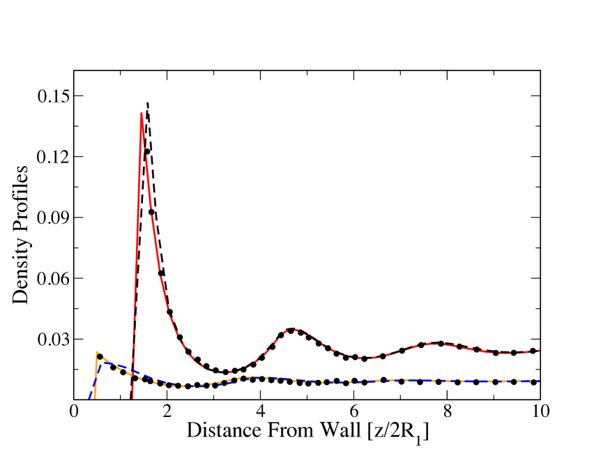
Figure 1: Reduced density profiles $8R_{1}^{3}\rho(z)$ versus the distance from the wall $z/2R_{1}$ of a binary hard-sphere mixture near a hard wall at diameter ratio $R_{2}/R_{1}=3$ and bulk reduced densities $0.0260$ and $0.0104$. The lines represent the 3D-FMT results using 3 or 6 grid points per hard-sphere diameter in the z-direction (dashed and solid lines, respectively). The black dots are the Monte-Carlo reference simulation data from Tan et al. tan_hardsphere_1989 .

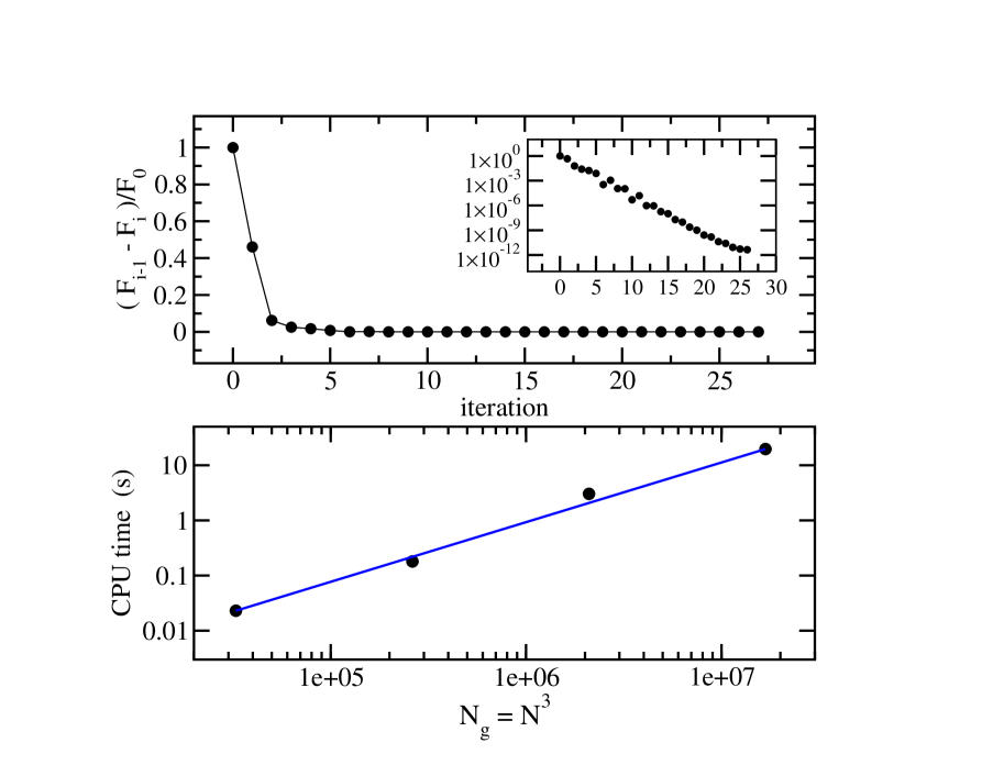
Figure 2: Top: Typical plot of the free energy difference between two successive steps (normalized by the initial energy) versus L-BFGS minimization-step number (Here a benzene molecule in a one-component HS reference fluid modeling SPC water; see Fig. 4). The inlet represents the same with a logarithmic scale in ordinates. Bottom: CPU time per minimization step versus number of 3D-grid points. The circle correspond in increasing order to N= 32, 64, 128, and 256.

IV Application to hydrophobic solvation

In continuation to previous works on molecular density functional theoryramirez02 ; ramirez05 ; ramirez05-CP ; gendre09 ; zhao11 ; borgis12 ; zhao-wu11 ; zhao-wu11-correction , we apply our implementation of KR-FMT to improve the MDFT description of molecular solutes in liquid water at ambient conditions (bulk density $\rho_{0}=0.03328$ molecules/$\AA^{3}$). In MDFT, the solvent response to the solute external field is described in terms of a functional of the inhomogeneous position and orientation density, $\rho(\mathbf{r},\Omega)$. If the solute is modeled as a purely hydrophobic entity, bearing no electrostatic multipole, and if the solvent position-orientation coupling is neglected (which is a good approximation for water), the angular dependence can be omitted, and the functional can be expressed in terms of the isotropic number density, $\rho(\mathbf{r})=\int d\Omega\,\rho(\mathbf{r},\Omega)$:

$${\cal F}[\rho(\mathbf{r})] = k_{B}T\int d\mathbf{r}\,\left[\rho(\mathbf{r})\ln\left(\frac{\rho(\mathbf{r})}{\rho_{0}}\right)-\rho(\mathbf{r})+\rho_{0}\right]$$ (18)

$$+\int d\mathbf{r}\,V(\mathbf{r})\rho(\mathbf{r})$$

$$-\frac{k_{B}T}{2}\int d\mathbf{r}d\mathbf{r}^{\prime}\Delta\rho(\mathbf{r})\,\Delta\rho(\mathbf{r}^{\prime})\,c_{S}(|\mathbf{r}-\mathbf{r}^{\prime}|;\rho_{0})$$

$$+{\cal F}_{B}[\rho(\mathbf{r})]$$

with $\Delta\rho(\mathbf{r})=\rho(\mathbf{r})-\rho_{0}$. $V(\mathbf{r})$ is the external potential to be defined below. The last two terms represent the excess free energy, ${\cal F}_{exc}[\rho(\mathbf{r})]$, which is decomposed into a homogeneous reference fluid (HRF) term, involving the isotropic direct correlation function of the pure solvent at the density $\rho_{0}$, $c_{S}(r;\rho_{0})$, and a correction term or ”bridge” term (in reference to integral equation theory), which is basically unknown, but can be formally expanded in terms of the pure solvent three-body,…, N-body direct correlation functions. The approximation that we propose here is rather standardrosenfeld93 ; biben98 ; zhao-wu11 and consists in replacing the unknown bridge for liquid water by the exact bridge of an equivalent hard-sphere fluid

$${\cal F}_{B}[\rho(\mathbf{r})] = {\cal F}_{exc}^{HS}[\rho(\mathbf{r})]-{\cal F}_{exc}^{HS}[\rho_{0}]-\mu_{exc}^{HS}\int d\mathbf{r}\Delta\rho(\mathbf{r})$$ (19)

$$+ \frac{k_{B}T}{2}\int d\mathbf{r}d\mathbf{r}^{\prime}\Delta\rho(\mathbf{r})\,\Delta\rho(\mathbf{r}^{\prime})\,c_{S}^{HS}(|\mathbf{r}-\mathbf{r}^{\prime}|;\rho_{0})$$

The first three terms represent the one-component hard-sphere KR-FMT excess functional defined in the previous section and the associated chemical potential yielding equilibrium at $\rho(\mathbf{r})=\rho_{0}$. The fourth term involves the direct correlation function of the HS fluid at the same density, i.e

$$c_{S}^{HS}(|\mathbf{r}-\mathbf{r}^{\prime}|;\rho_{0})=-\frac{\delta^{2}{\cal F}_{exc}^{HS}[\rho]}{\delta\rho(\mathbf{r})\delta\rho(\mathbf{r}^{\prime})}|_{\rho(\mathbf{r})=\rho_{0}}.$$ (20)

This function can be easily obtained in Fourier space as

$$c_{S}^{HS}(k;\rho_{0})=-\sum_{\alpha,\beta}\frac{\partial^{2}\Phi}{\partial n_{\alpha}\partial n_{\beta}}(\{n_{\gamma}^{0}\})\,\omega_{\alpha}(k)\omega_{\beta}(k)$$ (21)

where $\{n_{\gamma}^{0}\}$ represent the weighted densities for a uniform fluid of density $\rho_{0}$ and the $\omega_{\alpha,\beta}(k)$ are the weights of eq. 15. The second derivatives have to be taken for the PY or CS functions of eqs 16 or 17; the corresponding functions are reported in the Appendix. Note that defined as in eq. 19, ${\cal F}_{B}[\rho(\mathbf{r})]$ carries an expansion in $\Delta\rho$ of order 3 and higher that corrects the second order expansion of the excess free energy in eq. 18.

In this approach, two elements should be further defined. First the direct correlation of water. In principle it can be extracted from the experimental oxygen-oxygen structure factor. Since our further comparison will be with respect to molecular dynamics simulations carried out with the SPC water model, we have computed $c_{S}(r;\rho_{0})$ for this model. To do so we have re-generated the well-known oxygen-oxygen pair distribution function by carrying out molecular dynamics simulations with 4096 water molecules and a box size of $\sim 50\AA$; see Fig. 3. The corresponding direct correlation function can be deduced by solving the Ornstein-Zernike equation. This can be done quite naturally in Fourier-spacehansen . To avoid the numerical problems that occur in this case at small k-values, we have used instead the direct space method of Baxterbaxter70 combined with the variational method of Dixon and Hutchinsondixon77 ; see Ref. ramirez05-CP for details. This method imposes that the direct correlation function vanishes beyond a cut-off value that we set to $R_{c}=8.7\AA$. The corresponding function $c_{S}(r;\rho_{0})$ is plotted in Fig. 3. A second necessary ingredient is to fix the radius $R$ of the equivalent hard-sphere fluid. A natural value is around $R\simeq 1.25\AA$ that corresponds to the hard core, i.e. the region where $h_{S}(r)=0$ in Fig. 3. This choice can be confirmed by a striking fact noticed by Chandler and Varilly in Ref. chandler-varilly11 (see their figure 6): the statistics of spontaneous empty cavities in SPC water, that they tightly link in their Gaussian field analysis to the mechanism of hydrophobic solvation, are quite similar to those obtained for a hard-sphere liquid at a reduced density $\rho^{*}=8\rho_{0}R^{3}=0.5$, yielding $R\simeq 1.25\AA$ at the water density. Small variations around that value can be conceived and for reasons described below we were led to choose $R=1.27\AA$.

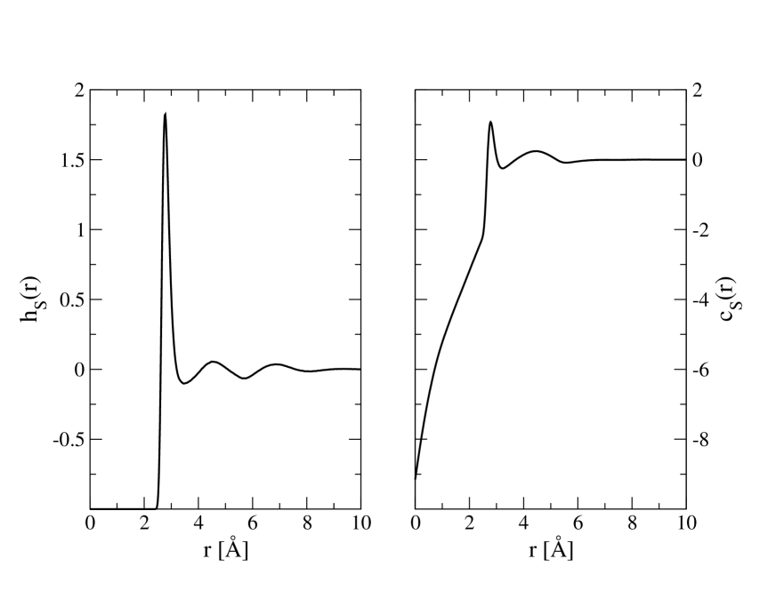
Figure 3: Left: Oxygen-oxygen isotropic pair distribution function of SPC water, $h_{S}(r)$, computed by molecular dynamics. Right: corresponding direct correlation function, $c_{S}(r)$, obtained by Ornstein-Zernike inversion using the Baxter direct-space method.

With the previous elements in hand, the functional of eqs 18-19 can be minimized in the external Lennard-Jones potential field imposed by a molecular solute placed at the center of a cubic box. It is defined as

$$V(\mathbf{r})=\sum_{i}4\epsilon_{wi}\left[\left(\frac{\sigma_{wi}}{|\mathbf{r}-\mathbf{r}_{i}|}\right)^{12}-\left(\frac{\sigma_{wi}}{|\mathbf{r}-\mathbf{r}_{i}|}\right]^{6}\right]$$ (22)

where the $\mathbf{r}_{i}$’s stand for the positions of the solute atomic sites and $\sigma_{wi},\epsilon_{wi}$ are the site-water Lennard-Jones parameters (using Lorentz-Berthelot mixing rules and the SPC parameters for water).

For the the KR-FMT excess free-energy terms, we have used either the PY or CS version, eqs 16 and  17 (with very little influence of this choice on the results, as will be seen). In addition to those terms that can be handled as described in the previous section, one needs to compute the $c_{S}$ and $c_{S}^{HS}$ quadratic terms; since they appear as convolutions, this is easily done by forward-backward Fourier transform as in a regular HRF approximationramirez02 . The procedure is illustrated in Fig. 4, representing the three-dimensional density obtained by minimization around a benzene molecule (Lennard-Jones parameters from Ref. laaksonen98 , no electrostatics). In Fig. 5, we compare the molecule site-water oxygen (C-O_w and H-O_w) pair distribution functions obtained by DFT with and without the bridge term of eq. 19 to the same quantities generated by molecular dynamics simulations (one solute and 512 SPC water molecules). Two features should be noted. First the bridge term turns out to have little influence on the overall microscopic structure, although it has a noticeable influence on the computed solvation free energies (see below). Secondly, the agreement to MD can be qualified as quite satisfactory, despite a disagreement in the shape of the first peak for C-O_w. The same type of comparison is drawn in Fig. 6 for propane. The geometry and parameters of Ashbaugh et al.ashbaugh_hydration_1998 were used with a unified description of the CH₂ and CH₃ groups. Again the agreement with the MD results is quite good, with a slight underestimation of the first peak width for CH₃-O_w. The influence of the bridge term on the structure remains marginal.

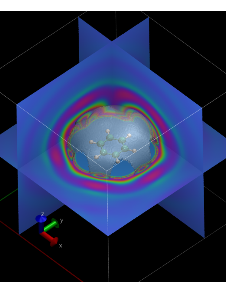
Figure 4: Three-dimensional representation of the reduced density of SPC water around a benzene molecule obtained by minimization of the functional. Blue to red indicate low to high densities up to $\rho(\mathbf{r})/\rho_{0}\simeq 3.5$. The transparent grey surface that appears above the molecule represents the isosurface $\rho(\mathbf{r})/\rho_{0}=2.0$.

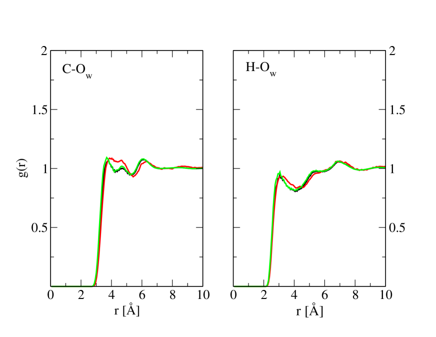
Figure 5: Site-oxygen radial distribution functions for a benzene molecule in SPC water: MD results (red line) compared to the DFT results with and without the HS bridge term with $R=1.27\AA$ (black and green lines, respectively).

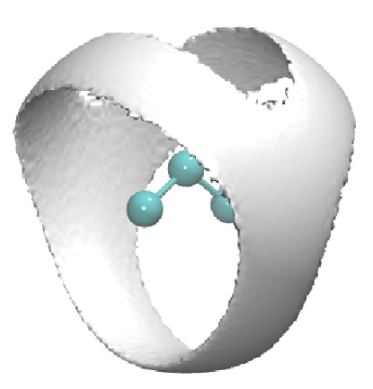
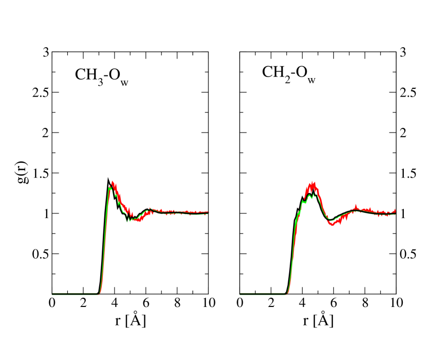
Figure 6: Site-oxygen radial distribution functions for a propane molecule in SPC water: MD results (red line) compared to the DFT results with and without the HS bridge term with $R=1.27\AA$ (black and green lines, respectively). The top figure is a representation of the molecule and of the solvent reduced density isosurface corresponding to $\rho(\mathbf{r})/\rho_{0}=2.0$.

Finally Table 1 compares the solvation free energies obtained for a series of rare-gas atoms and alcanes molecules to the MD results reported by Guillot and Guissani using a particle insertion methodguillot_guissani_1993 or Ashbaugh et al. using thermodynamic integration techniquesashbaugh_hydration_1998 . It is seen that the straight application of the HRF approximation, ${\cal F}_{B}[\rho]=0$, systematically overestimate the solvation free-energies. In Fig. 7 we display the free-energy energy of methane obtained when adding the hard-sphere bridge term of eq. 19 and varying the hard-sphere radius around $1.25\AA$. It can be observed that the computed free-energy decreases steadily with increasing $R$ (whereas the microscopic water structure remains unaffected by the added bridge term in this parameter range, see Figs 5 and  6). Furthermore we show that using either the CS or PY version of the HS functional has a very small –although measurable– effect on the results. Retaining the CS version, we find that the MD value for methane in Table 1 is reached when $R\simeq 1.27\AA$. Keeping that value, we find a close correlation to the MD results for the whole series of molecules. These encouraging findings are listed in Table 1 and further depicted in Fig. 8. Note that for each point in the figure, the computational effort to get the solvation free energy is orders of magnitude lower for 3D-DFT than for MD.

Molecule	MD	DFT/HRF	DFT/HRF+bridge
methane	10.96$\pm 0.46$	16.03	10.43
ethane	10.75$\pm 0.50$	18.50	10.33
propane	13.81$\pm 0.54$	24.86	13.64
butane	14.69$\pm 0.54$	28.56	14.71
pentane	15.43$\pm 0.59$	32.23	15.87
hexane	16.40$\pm 0.63$	35.99	17.02
Ne	11.21$\pm 0.46$	14.47	11.67
Ar	8.661$\pm 0.46$	14.04	9.51
Kr	8.242$\pm 0.46$	14.68	9.20

Table 1: Solvation free energies of rare-gas atoms and alcane molecules in SPC water computed by DFT using the HRF approximation (eq. 18 with ${\cal F}_{B}=0$) or the HRF + hard-sphere bridge approximation (eqs 18 and eq. 19 with $R=1.27\AA$). They are compared to the MD values of Ref. ashbaugh_hydration_1998 for alcanes and Ref. guillot_guissani_1993 for rare gases (with the corresponding error bars). All values are in kJ/mol.

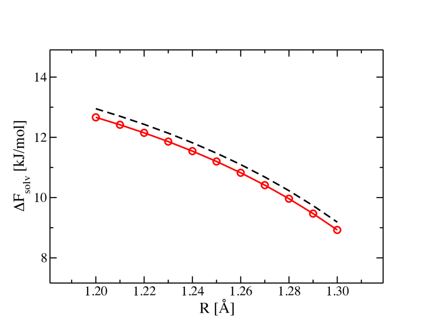
Figure 7: Hydration free energy versus reference hard-sphere radius for methane, using either the Percus-Yevick (red circles and line) or Carnahan-Starling (black dashed line) versions of the FMT functional for the bridge term (eq. 19).

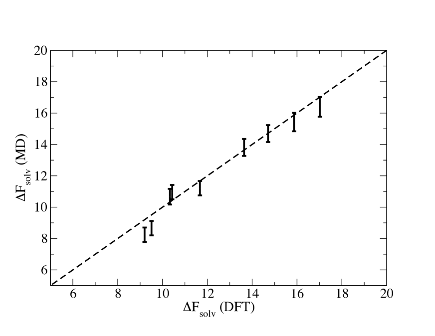
Figure 8: Comparison of the free energy of hydration for rare gases and alcanes (in trans conformation), calculated either by DFT with a hard-sphere bridge function of radius $1.27\AA$ or by MD simulations (Refs ashbaugh_hydration_1998 and guillot_guissani_1993 ). From left to right: Kr, Ar, ethane, methane, propane, Ne, butane, pentane, hexane. The vertical bars correspond to the MD error bars indicated in Table 1. Units are kJ/mol.

V Conclusion

This paper has presented the first three-dimensional implementation, to our knowledge, of the Kierlik-Rosinberg fundamental measure theory for hard-sphere mixtures. Since the free-energy is written in terms of convolutions of the microscopic density with respect to discontinuous weight functions, the FMT density functionals are reputed to require very fine grids and very long recursive minimizations, at least for low dimensional applications. In the three-dimensional case, we showed that using discrete 3D-FFT’s which are well suited to describe the convolution of smooth functions with discontinuous (step-like or delta-like) distributions and using a more elaborated minimizer that the Picard iteration scheme that is usually prescribedroth-review10 , the Kierlik-Rosinberg FMT functional can be efficiently minimized for realistic systems with a grid resolution of only a few points per Angstrom and within at most a few tens of iterations. Such implementation constitutes a basis for tackling very diverse problems in physical chemistry involving fluids or solutions in the presence of atomistically-resolved interfaces or confinement matrices. To describe realistic interactions, dispersive and Coulombic contributions can be easily introduced as mean field perturbations to the hard-core functionalbiben98 ; oleksy10 . We are working presently on several applications in that context.

We have used here the implementation for another purpose: try to infer N-body corrections in the molecular density functional theory description of water, a system for which the restriction to two-body correlations (the so called homogeneous reference fluid approximation or HNC approximation in an integral equation context) was found to present shortcomingsrichardi98 ; zhao11 . Hard-sphere corrections do seem to help for the special but important case of hydrophobic solvation. As stated in the introduction, however, the present approach is meant to describe hydrophobicity at microscopic length scales but not to account properly for macroscopic phenomena such as dewettinglum99 ; chandler02 ; varilly11 . Such limitation could be bypassed by adding coarse-grained contributions to the microscopic short-ranged functional.

Furthermore the present effort has to be continued for the general situation of polar and charged solutes, for which electrostatic interactions and solvent angular dependence have to be included. In that case, despite positive results when MDFT is used as a post-treatment of exact densitieszhao-wu11 ; zhao-wu11-correction , we have some preliminary indications, and there are premises in the literature toorichardi99 ; lombardero99 ; reddy03 , that life might not be so simple with self-consistent minimization, and that angular-independent bridge corrections might not be sufficient. Mixing the type of hard-sphere corrections studied here to the H-bonding three-body corrections introduced in Ref. zhao11 might be a way out.

Appendix A A few useful formulas

The first derivatives of the function $\Phi(\{n_{\alpha}\})$ in eq. 6 with respect to the weighted densities are required to compute the functional gradients and perform the minimization (see the Euler-Lagrange equation, eq. 9). The second derivatives make it possible to compute the hard-sphere direct correlation functions, eq. 21. They are required too if a Newton-like minimization algorithm such as GMRESsaad86 ; sears03 is used instead of L-BFGS (which is quite efficient but memory demanding).

All those derivatives are listed below for the PY version of KR-FMT, eq. 16:

$$\frac{\partial\Phi^{PY}}{\partial n_{0}} = -\ln(1-n_{3})$$

$$\frac{\partial\Phi^{PY}}{\partial n_{1}} = \frac{n_{2}}{1-n_{3}}$$

$$\frac{\partial\Phi^{PY}}{\partial n_{2}} = \frac{n_{1}}{1-n_{3}}+\frac{n_{2}^{2}}{8\pi(1-n_{3})^{2}}$$

$$\frac{\partial\Phi^{PY}}{\partial n_{3}} = \frac{n_{0}}{1-n_{3}}+\frac{n_{1}n_{2}}{(1-n_{3})^{2}}+\frac{n_{2}^{3}}{12\pi(1-n_{3})^{3}}$$

$$\frac{\partial^{2}\Phi^{PY}}{\partial n_{0}\partial n_{3}} = \frac{\partial^{2}\Phi^{PY}}{\partial n_{1}\partial n_{2}}=\frac{1}{1-n_{3}}$$ (23)

$$\frac{\partial^{2}\Phi^{PY}}{\partial n_{1}\partial n_{3}} = \frac{n_{2}}{(1-n_{3})^{2}}$$

$$\frac{\partial^{2}\Phi^{PY}}{\partial n_{2}^{2}} = \frac{n_{2}}{4\pi(1-n_{3})^{2}}$$

$$\frac{\partial^{2}\Phi^{PY}}{\partial n_{2}\partial n_{3}} = \frac{n_{1}}{(1-n_{3})^{2}}+\frac{n_{2}^{2}}{4\pi(1-n_{3})^{3}}$$

$$\frac{\partial^{2}\Phi^{PY}}{\partial n_{3}^{2}} = \frac{n_{0}}{(1-n_{3})^{2}}+\frac{2n_{1}n_{2}}{(1-n_{3})^{3}}+\frac{n_{2}^{3}}{4\pi(1-n_{3})^{4}}$$

and for the CS version, eq. 16:

$$\frac{\partial\Phi^{CS}}{\partial n_{0}} = -\ln(1-n_{3})$$

$$\frac{\partial\Phi^{CS}}{\partial n_{1}} = \frac{n_{2}}{1-n_{3}}$$

$$\frac{\partial\Phi^{CS}}{\partial n_{2}} = \frac{n_{1}}{1-n_{3}}+\frac{n_{2}^{2}}{12\pi(1-n_{3})^{2}n_{3}}+\frac{n_{2}^{2}}{12\pi n_{3}^{2}}\ln(1-n_{3})$$

$$\frac{\partial\Phi^{CS}}{\partial n_{3}} = \frac{n_{0}-n_{2}^{3}/(36\pi n_{3}^{2})}{1-n_{3}}+\frac{n_{1}n_{2}}{(1-n_{3})^{2}}-\frac{n_{2}^{3}}{36\pi(1-n_{3})^{2}n_{3}^{2}}$$

$$+\frac{n_{2}^{3}}{18\pi n_{3}(1-n_{3})^{3}}-\frac{n_{2}^{3}}{18\pi n_{3}^{3}}\ln(1-n_{3})$$

$$\frac{\partial^{2}\Phi^{CS}}{\partial n_{0}\partial n_{3}} = \frac{\partial^{2}\Phi^{CS}}{\partial n_{1}\partial n_{2}}=\frac{1}{1-n_{3}}$$ (24)

$$\frac{\partial^{2}\Phi^{CS}}{\partial n_{1}\partial n_{3}} = \frac{n_{2}}{(1-n_{3})^{2}}$$

$$\frac{\partial^{2}\Phi^{CS}}{\partial n_{2}^{2}} = \frac{n_{2}}{6\pi n_{3}(1-n_{3})^{2}}+\frac{n_{2}}{6\pi n_{3}^{2}}\ln(1-n_{3})$$

$$\frac{\partial^{2}\Phi^{CS}}{\partial n_{2}\partial n_{3}} = -\Big{(}n_{3}(n_{2}^{2}(2-5n_{3}+n_{3}^{2})-12\pi n_{1}(1-n_{3})n_{3}^{2})$$

$$+2n_{2}^{2}(1-n_{3})^{3}\ln(1-n_{3})\Big{)}/(12\pi(1-n_{3})^{3}n_{3}^{3})$$

$$\frac{\partial^{2}\Phi^{CS}}{\partial n_{3}^{2}} = \Big{(}n_{3}(n_{2}^{3}(6-21n_{3}+26n_{3}^{2}-5n_{3}^{3})+72\pi n_{1}n_{2}(1-n_{3})n_{3}^{3}$$

$$+36\pi n_{0}(1-n_{3})^{2}n_{3}^{3})+6n_{2}^{3}(1-n_{3})^{4}\ln(1-n_{3})\Big{)}$$

$$/(36\pi(1-n_{3})^{4}n_{3}^{4})$$

All the second derivatives that are not written are equal to zero. There are thus 6 non-vanishing second derivatives to be considered instead of 21 in the Rosenfeld’s vectorial versionsears03 . In this respect also, the Kierlik-Rosinberg version of FMT appears much simpler to manipulate and will be more efficient in Newton-like minimization schemes.

References

- (1) J. P. Hansen and I. R. McDonald, Theory of Simple Liquids, Academic Press, London, 1989.
- (2) C. G. Gray and K. E. Gubbins, Theory of Molecular Fluids, Volume 1: Fundamentals, Clarendon Press, Oxford, 1984.
- (3) D. Chandler and H. Hendersen, J. Chem. Phys. 57, 1930 (1972).
- (4) F. Hirata and P. J. Rossky, Chem. Phys. Lett. 83, 329 (1981).
- (5) F. Hirata, B. M. Pettitt, and P. J. Rossky, J. Chem. Phys. 77, 509 (1982).
- (6) G. Reddy, C. P. Lawrence, J. L. Skinner, and A. Yethiraj, J. Chem. Phys. 119, 13012 (2003).
- (7) K. M. Dyer, J. S. Perkyns, and B. M. Pettitt, J. Chem. Phys. 127, 194506 (2007).
- (8) K. M. Dyer, J. S. Perkyns, G. Stell, and B. M. Pettitt, J. Chem. Phys. 129, 104512 (2008).
- (9) L. Blum and A. J. Torruella, J. Chem. Phys. 56, 303 (1972).
- (10) L. Blum, J. Chem. Phys. 57, 1862 (1972).
- (11) G. N. Patey, Mol. Phys. 34, 427 (1977).
- (12) S. L. Carnie and G. N. Patey, Mol. Phys. 47, 1129 (1982).
- (13) P. H. Fries and G. N. Patey, J. Chem. Phys. 82, 429 (1985).
- (14) J. Richardi, P. H. Fries, and H. Krienke, J. Chem. Phys. 108, 4079 (1998).
- (15) J. Richardi, C. Millot, and P. H. Fries, J. Chem. Phys. 110, 1138 (1999).
- (16) R. Evans, Adv. Phys. 28, 143 (1979).
- (17) R. Evans, in Fundamental of Inhomogeneous Fluids, edited by D. Henderson, New York, 1992, Marcel Dekker.
- (18) J. Wu and Z. Li, Ann. Rev. Phys. Chem. 58, 85 (2007).
- (19) D. Chandler, Phys. Rev. E 48, 2898 (1993).
- (20) P. R. ten Wolde, S. X. Sun, and D. Chandler, Phys. Rev. E 65, 011201 (2001).
- (21) R. D. Coalson and A. Duncan, J. Phys. Chem. B 100, 2612 (1996).
- (22) C. G. Gray, K. E. Gubbins, and C. J. Joslin, Theory of Molecular Fluids, Volume2: Applications, Clarendon Press, Oxford, 2011.
- (23) J. Wu, AIChE Journal 52, 1169 (2006).
- (24) D. Beglov and B. Roux, J. Phys. Chem. B 101, 7821 (1997).
- (25) A. Kovalenko and F. Hirata, Chem. Phys. Lett. 290, 237 (1998).
- (26) E. F. Hirata, Molecular Theory of Solvation, Kluwer Academic Publishers, Dordrecht, 2003.
- (27) N. Yoshida, T. Imai, S. Phongphanphanee, A. Kovalenko, and F. Hirata., J. Phys. Chem. B (2009).
- (28) T. Kloss and S. M. Kast, J. Chem. Phys. 128, 134505 (2008).
- (29) T. Kloss, J. Heil, and S. M. Kast, J. Phys. Chem. B 112, 4337 (2008).
- (30) R. Ramirez, R. Gebauer, M. Mareschal, and D. Borgis, Phys. Rev. E 66, 306 (2002).
- (31) R. Ramirez and D. Borgis, J. Phys. Chem. B 109, 6754 (2005).
- (32) R. Ramirez, M. Mareschal, and D. Borgis, Chem. Phys. 319, 261 (2005).
- (33) L. Gendre, R. Ramirez, and D. Borgis, Chem. Phys. Lett. 474, 366 (2009).
- (34) S. Zhao, R. ramirez, R. Vuilleumier, and D. Borgis, J. Chem. Phys. 134, 194102 (2011).
- (35) D. Borgis, D. gendre, and R. Ramirez, J. Phys. Chem. B 116, 2504 (2012).
- (36) S. Zhao, Z. Jin, and J. Wu, J. Phys. Chem. B 115, 6971 (2011).
- (37) S. Zhao, Z. Jin, and J. Wu, J. Phys. Chem. B 115, 15445 (2011).
- (38) C. Azuara, E. Lindahl, and P. Koehl, Nucleic Ac. Res. 34, 38 (2006).
- (39) C. Azuara, H. Orland, M. Bon, P. Koehl, and M. Delarue, Biophys. J. 95, 5587 (2008).
- (40) P. Varilly, A. J. Patel, and D. Chandler, J. Chem. Phys. 134, 074109 (2010).
- (41) J. K. Percus, J. Stat. Phys. 15, 505 (1976).
- (42) T. K. Vanderlick, H. T. Davis, and J. K. Percus, J. Chem. Phys. 91, 7136 (1989).
- (43) P. Tarazona and R. Evans, Mol. Phys. 52, 847 (1984).
- (44) P. Tarazona, Mol. Phys. 52, 81 (1984).
- (45) Y. Rosenfeld, Phys. Rev. Lett. 63, 980 (1989).
- (46) E. Kierlik and M. L. Rosinberg, Phys. Rev. A 42, 3382 (1990).
- (47) E. Kierlik and M. L. Rosinberg, Phys. Rev. A 44, 5025 (1991).
- (48) S. Phan, E. Kierlik, M. L. Rosinberg, B. Bildstein, and G. Kahl, Phys. Rev. E 48, 618 (1993).
- (49) R. Ohnesorge, H. Lowen, and H. Wagner, Europhys. Lett. 22, 245 (1993).
- (50) Y. Rosenfeld, M. Schmidt, H. Lowen, and P. Tarazona, J. Phys.: Condens. Matter 8, L577 (1996).
- (51) Y. Rosenfeld, M. Schmidt, H. Lowen, and P. Tarazona, Phys. Rev. E 55, 4245 (1997).
- (52) B. Groh and B. Mulder, Phys. Rev. E 61, 3811 (2000).
- (53) B. Groh, Phys. Rev. E 61, 5218 (2000).
- (54) P. Tarazona, Phys. Rev. Lett. 84, 694 (2000).
- (55) P. Tarazona, Physica A 306, 243 (2002).
- (56) J. A. Cuesta, Y. Martinez-Raton, and P. Tarazona, J. Phys.: Condens. Matter 14 (2002) 14, 11965 (2002).
- (57) J. F. Lutsko, Phys. Rev. E 74, 021121 (2006).
- (58) R. Roth, R. Evans, A. Lang, and G. Kahl, J. Phys. : Condens. Matter 14, 12063 (2002).
- (59) Y. X. Yu and J. Wu, J. Chem. Phys. 117, 10156 (2002).
- (60) J. Wu, in Molecular Thermodynamics of Complex Systems, edited by X. Lu and Y. Hu, Springer, 2009.
- (61) R. Roth, J. Phys.: Condens. Matter 22, 063102 (2010).
- (62) Y. Yu and J. Wu, J. Chem. Phys. 117, 2368 (2002).
- (63) Z. Jin, S. Zhao, and J. Wu, Phys. Rev. E 82, 041805 (2010).
- (64) A. Oleksy and J. P. Hansen, J. Chem. Phys. 132, 204702 (2010).
- (65) T. Jiang, D. Jiang, Z. Jin, and D. Henderson, Soft Matt. 7, 11222 (2011).
- (66) J. Jiang, D. Meng, and J. Wu, Chem. Phys. Lett. 504, 153 (2011).
- (67) M. G. Knepley, D. A. Karpeev, S. Davidovits, R. S. Eisenberg, and D. Gillespie, J. Chem. Phys. 132, 124101 (2010).
- (68) L. J. D. Frink and A. G. Salinger, J. Comput. Phys. 159, 407 (2000).
- (69) M. P. Sears and L. J. D. Frink, J. of Comp. Phys. 190, 184 (2003).
- (70) V. Molinero and E. B. Moore, J. Phys. Chem. B 113, 4008 (2009).
- (71) F. Lado, Phys. Rev. A 8, 2548 (1976).
- (72) Y. Rosenfeld, J. Chem. Phys. 98, 8126 (1993).
- (73) K. Lum, D. Chandler, and J. D. Weeks, J. Phys. Chem. B 103, 4570 (1999).
- (74) D. Chandler, Nature 417, 491 (2002).
- (75) D. Chandler and P. Varilly, Lectures on molecular- and nano-scale fluctuations in water, in Complex materials in physics and biology, arXiv: 1101:2235, 2010.
- (76) N. Giovambattista, F. L. Carlos, P. J. Rossky, and P. G. Debenedetti, Proc. Nat. Acad. Sci. USA 105, 2274 (2008).
- (77) N. Giovambattista, P. G. Debenedetti, and P. J. Rossky, Proc. Nat. Acad. Sci. USA 106, 15181 (2009).
- (78) S. Matysiak, P. G. Debenedetti, and P. J. Rossky, J. Phys. Chem. B 115, 14859 (2011).
- (79) L. R. Pratt and D. Chandler, J. Chem. Phys. 67, 3683 (1977).
- (80) S. Phan, E. Kierlik, M. L. Rosinberg, B. Bildstein, and G. Kahl, Physical Review E 48, 618 (1993).
- (81) R. H. Byrd, P. Lu, and J. Nocedal, SIAM J. Scient. Stat. Comp. 16, 1190 (1995).
- (82) Z. Tan, U. M. B. Marconi, F. van Swol, and K. E. Gubbins, J. Chem. Phys. 90, 3704 (1989).
- (83) T. Biben, J. P. Hansen, and Y. Rosenfeld, Phys. Rev. E 57, R3727 (1998).
- (84) R. J. Baxter, J. Chem. Phys. 52, 4559 (1970).
- (85) M. Dixon and P. Hutchinson, Mol. Phys. 33, 1663 (1977).
- (86) A. Laaksonen, P. Stilbs, and R. E. Wasylishen, J. Chem. Phys. 108, 455 (1998).
- (87) H. S. Ashbaugh, E. W. Kaler, and M. E. Paulaitis, Biophysical Journal 75, 755 (1998).
- (88) B. Guillot and Y. Guissani, The Journal of Chemical Physics 99, 8075 (1993).
- (89) M. Lombardero, C. martin, S. Jorge, F. Lado, and E. Lomba, J. Chem. Phys. 110, 1148 (1999).
- (90) Y. Saad and M. Schultz, SIAM J. Sci. Stat. Comp. 7, 856 (1986).