Exactly solvable balanced tenable urns with random entries via the analytic methodology

Abstract

This paper develops an analytic theory for the study of some Pólya urns with random rules. The idea is to extend the isomorphism theorem in Flajolet et al. (2006), which connects deterministic balanced urns to a differential system for the generating function. The methodology is based upon adaptation of operators and use of a weighted probability generating function. Systems of differential equations are developed, and when they can be solved, they lead to characterization of the exact distributions underlying the urn evolution. We give a few illustrative examples.

1 Introduction

A classical definition of the Pólya urn scheme specifies it as an urn which contains balls of up to two colors (say black and white), and which is governed by a set of evolution rules. A step then consists in randomly picking a ball from the urn, placing it back, and depending on its color, adding or discarding a fixed number of black and white balls.

Flajolet et al. (2006) introduces an analytic method to deal with a class of two-color Pólya urns with deterministic addition rules. The method leads to a fundamental connection to differential equations via an isomorphism theorem. In the present manuscript, we extend the method to deal with Pólya urns with random addition rules. One can think of schemes with random replacements as mixtures of deterministic schemes, with appropriate probabilities.

We develop an analytic theory for the study of balanced tenable Pólya urns with random rules (we shall make the terms “balanced” and “tenable” more precise in Section 2). Balance and tenability are restrictions on the rules that admit an analytic treatment through generating functions. Our main result is the following: to each system of random rules satisfying the balance and tenability conditions, one can associate a differential system which describes the generating function counting the sequence of configurations of the urn scheme. A formal statement of this theorem appears in Section 3.

When the system can be solved, it leads to characterization of the exact distributions underlying the urn evolution. In Section 4, we give some examples where the generating function is explicit. Some of them include uniform and binomial discrete random variable in their rules. Other examples investigate some coupon collector variants. Finding the generating function and deducing the probability distributions is quite mechanical, owing to classical analytic combinatorics.

2 Basic definitions

In Pólya’s classical urn model, we have an urn containing balls of up to two different colors, say black and white. The system evolves with regards to particular evolution rules: at each step, add (possibly a negative number) black and white balls. These rules are specified by a $2\times 2$ matrix:

$$\begin{pmatrix}\alpha&\beta\\ \gamma&\delta\end{pmatrix},\qquad\alpha,\delta\in\mathbb{Z}\,,\quad\beta,\gamma\in\mathbb{Z}_{\geq 0}\,.$$ (1)

The rows of the matrix are indexed with the colors black and white respectively. The columns of the matrix are indexed by the same colors: they are from left to right indexed by black and white.

The asymptotics of this construct have been approached by traditional probabilistic methods in Athreya and Karlin (1968), Smythe (1996) and Janson (2004). Mahmoud (2008) presents some of these findings.

In this manuscript we deal with a model where the constants $\alpha$, $\beta$, $\gamma$, and $\delta$ are replaced by random variables. We attempt to provide an approach for the study of the urn’s composition after a finite, and possibly small, number of ball draws. This is an equally important line of attack and can be viewed as more important in practice, when the number of draws is not sufficiently large to warrant approximation by asymptotics. We focus on exact distributions in this paper.

2.1 Balanced tenable urns with random entries

We consider urns for which the dynamics of change are now represented by the replacement matrix

$$\begin{pmatrix}\mathcal{A}&\mathcal{B}\\ \mathcal{C}&\mathcal{D}\end{pmatrix},$$ (2)

where $\mathcal{A},\mathcal{B},\mathcal{C}$ and $\mathcal{D}$ are discrete random variables. If a random variable has a negative realization, it means we discard balls.

Let $B_{n}$ and $W_{n}$ be respectively the number of black and white balls after $n$ draws from the urn. We call the pair $(B_{n},W_{n})$ the configuration of the urn after $n$ steps (draws). We start with a deterministic initial configuration $(B_{0},W_{0})=(\cramped{b_{0}},\cramped{w_{0}})$. At each step, a ball is uniformly drawn from the urn. We look at its color and we put it back in the urn: if the color is black, we add $\mathcal{A}$ black balls and $\mathcal{B}$ white balls; if the color is white, we add $\mathcal{C}$ black and $\mathcal{D}$ white balls; the random variables are generated independently at each step.

We now recall a few definitions, that serve to delineate the scope of our study.

Definition 2.1 (Balance)

An urn with the replacement matrix (2) is said to be balanced, if the sums across rows are equal, that is if $\mathcal{A}+\mathcal{B}=\mathcal{C}+\mathcal{D}$, and these sums are always constant and equal to a fixed value $\theta$. The parameter $\theta$ is called the balance of the urn.

All urns considered in this paper are balanced. As a consequence, the random variables are governed by the relations $\mathcal{B}=\theta-\mathcal{A}$, and $\mathcal{C}=\theta-\mathcal{D}$. In addition, we will only consider urns with nonnegative balance, $\theta\geq 0$. The case $\theta<0$ refers to diminishing urn models. Questions and results on these models are completely different; see Hwang et al. (2007) for an analytic development.

Since we allow the random variables $\mathcal{A}$ and $\mathcal{D}$ to take negative integer values, it is necessary to consider the concept of tenability.

Definition 2.2 (Tenability)

An urn scheme is said to be tenable, if it is always possible to apply a rule, i.e., if it never reaches a deadlocked configuration (that is, choosing with positive probability a rule that cannot be applied because there are not enough balls).

To illustrate this notion, suppose we have an urn of black and white balls, with the replacement matrix

$$\begin{pmatrix}-2&2\\ 2&-2\end{pmatrix}.$$

This matrix, together with an even initial number of black balls and an even initial number of white balls form a tenable scheme. Any other initial condition makes this scheme untenable. For instance, if we start with two black balls and one white ball, the scheme gets stuck upon drawing a white ball.

Remark 2.1

A tenable balanced urn scheme cannot have negative realizations for the nondiagonal entries $\mathcal{B}=\theta-\mathcal{A}$ and $\mathcal{C}=\theta-\mathcal{D}$, and they cannot have unbounded supports, either. Indeed, if $\mathcal{B}$ has a negative realization, say $-k$ for positive $k$, we discard $k$ white balls upon withdrawing a black ball. In view of the balance condition, we must add at the same step $\theta+k$ black balls; we can apply this rule repeatedly until we take out all white balls, and the scheme comes to a halt (contradicting tenability). Therefore, $\mathcal{B}$ and $\mathcal{C}$ must have only nonnegative realizations. Furthermore, suppose the urn at some step has $N$ black balls; if $\mathcal{B}$ has an unbounded support, it includes a value greater than $\theta+N$. Here $\mathcal{A}$ must realize a value less then $-N$. A draw of a black ball requires taking out more than $N$ black balls (contradicting tenability).

Example 2.1

This example illustrates a mixed model urn in the class we are considering. It has random entries in the replacement matrix and is balanced and tenable. Consider the Pólya-Friedman urn scheme with the replacement matrix

$$\begin{pmatrix}\mathcal{B}_{p}&1-\mathcal{B}_{p}\\ 1-\mathcal{B}_{p}&\mathcal{B}_{p}\end{pmatrix},$$ (3)

where $\mathcal{B}_{p}$ is a Ber($p$) random variable. Such a scheme has balance one, and alternates between

$$\begin{pmatrix}1&0\\ 0&1\end{pmatrix},\qquad\textmd{and}\qquad\begin{pmatrix}0&1\\ 1&0\end{pmatrix},$$

that is between Pólya-Eggenberger’s urn (with probability $p$) and Friedman’s urn (with probability $1-p$). The transition in the limit distribution of black balls when $p$ goes from 0 to 1 is quite unusual. For $p=0$ (Friedman’s urn), a properly normalized number of black balls has the classical Gaussian distribution, and for $p=1$ (Pólya-Eggenberger’s urn), a properly scaled number of black balls has a beta distribution. The scheme with replacement matrix (3) is an interesting example that warrants further investigation, and will be a special case of two illustrative examples (Subsections 4.2 and 4.3).

2.2 Definitions for the analytic methodology

The first use of analytic combinatorics for the treatment of urn models is in Flajolet et al. (2005), where some balanced urns are linked to a partial differential equation and elliptic functions. We now describe the analytic tools we use for our study. For a more complete (yet accessible) account see Morcrette (2012) (§2). For a precise overview of analytic combinatorics, see the reference book Flajolet and Sedgewick (2009).

The total number of balls after $n$ draws, denoted by $\cramped{s_{n}:=B_{n}+W_{n}}$, is deterministic because of the balance condition. Indeed, at each step, we add a constant number of balls (the balance $\theta$), so

$$s_{n}=s_{0}+\theta n=b_{0}+w_{0}+\theta n\,.$$ (4)

The main tool in this study is the weighted probability generating function

$$Q(x,y,z):=\sum_{n=0}^{\infty}\sum_{b,w\geq 0}s_{0}s_{1}\ldots s_{n-1}\,{\mathbb{P}}(B_{n}=b,W_{n}=w)\,x^{b}y^{w}\,\frac{z^{n}}{n!}\,.$$ (5)

The variable $x$ counts black balls, $y$ counts white balls, and $z$ counts the number of draws. As $b$, $w$ and $n$ are governed by (4), one of the variables is redundant. So we can set $y=1$ without loss of generality: it is sufficient to study a marginal distribution because it determines the joint probability distribution.

Remark 2.2

The kernel $\cramped{s_{0}s_{1}\ldots s_{n-1}}$ corresponds to the total number of paths of length $n$ starting from the initial configuration. Indeed, at step 0 we can pick a ball among the $s_{0}$ balls in the urn; at step 1 we can pick a ball among the $s_{1}$ balls in the urn, etc.

Remark 2.3

The coefficient $\cramped{[x^{b}y^{w}z^{n}/n!]}Q(x,y,z)$ does not represent a combinatorial count; this quantity can be fractional. Nevertheless, it is closely connected to the notion of “history” described in Flajolet et al. (2006). A history is nothing but a finite sequence of draws from the urn. One history of length $n$ describes one possible evolution from step $0$ to step $n$. It can be viewed as a path in the evolution tree of the urn. In the context of deterministic rules, histories are combinatorial counts. However, in our case, we need more information to have a complete description of a sequence of $n$ draws. At each step, we can choose different rules depending on the realization of the random entries at that step. So, we are now dealing with weighted histories, that is the sequence of $n$ draws with a weight factor corresponding to the probability of applying the $n$ different rules we use along the path from step $0$ to step $n$. If we denote by $\cramped{Q_{n,b,w}}$ the contribution of weighted histories beginning at step $0$ in the configuration $(b_{0},w_{0})$ and ending at step $n$ in the configuration $(b,w)$, we have

$$Q(x,y,z)=\sum_{n=0}^{\infty}\sum_{b,w\geq 0}Q_{n,b,w}\,x^{b}y^{w}\frac{z^{n}}{n!}\,.$$ (6)

The kernel $\cramped{s_{0}s_{1}\ldots s_{n-1}}$ is obtained by adding all weighted histories of length $n$, that is by setting $x$ and $y$ to 1:

$$Q(1,1,z)=(1-\theta z)^{-s_{0}/\theta}\,;\qquad n!\,[z^{n}]Q(1,1,z)=s_{0}s_{1}\ldots s_{n-1}=\theta^{n}\,\frac{\Gamma(n+s_{0}/\theta)}{\Gamma(s_{0}/\theta)}\,.$$

In this way, we preserve the equivalence between the probabilistic model and the combinatorial aspects of weighted history. The balance condition is key to this equivalence:

$${\mathbb{P}}(B_{n}=b,W_{n}=w)=\frac{\left[x^{b}y^{w}z^{n}\right]Q(x,y,z)}{\left[z^{n}\right]Q(1,1,z)}=\frac{Q_{n,b,w}}{s_{0}\ldots s_{n-1}}\,.$$ (7)

3 An isomorphism theorem for urn schemes with random entries

In this section, we state our main result through the following theorem which links the behavior of a tenable balanced urn to a differential system. The theorem always yields a differential system, and the difficulty then lies in extracting information on the generating function: indeed, the system obtained may not be always explicitly solvable by currently known techniques.

Theorem 3.1

Given a balanced tenable urn with the replacement matrix

$$\begin{pmatrix}\mathcal{A}&\theta-\mathcal{A}\\ \theta-\mathcal{D}&\mathcal{D}\end{pmatrix},$$

where $\mathcal{A}$ and $\mathcal{D}$ are discrete random variables with distributions

$${\mathbb{P}}(\mathcal{A}=k)=\pi_{k}\,,\qquad{\mathbb{P}}(\mathcal{D}=k)=\tau_{k}\,,$$

for $-K\leq k\leq\theta$, (for some $K>0$), the probability generating function of the urn is given by

$$Q\left(x,y,z\right)=X^{b_{0}}(z)\,Y^{w_{0}}(z)\,,$$

where $(b_{0},w_{0})$ is the starting configuration, and the pair $(X(t)\,,Y(t))$ is the solution to the differential system

$$\left\{\begin{array}[]{ccc}x^{\prime}(t)&=&\displaystyle\sum_{k=-K}^{\theta}\pi_{k}\,x^{k+1}(t)\,y^{\theta-k}(t)\,;\\ y^{\prime}(t)&=&\displaystyle\sum_{k=-K}^{\theta}\tau_{k}\,x^{\theta-k}(t)\,y^{k+1}(t)\,,\end{array}\right.$$

applied at $t=0$, and any initial conditions $x:=x(0)\textrm{ and }y:=y(0)$, such as $xy\not=0$.

The proof follows and generalizes that in Flajolet et al. (2006). The basic idea in this proof is that the monomial $\cramped{x^{i}y^{j}}$ represents the configuration $\cramped{(B_{n},W_{n})=(i,j)}$. The actions of the urn transform such a configuration into $\cramped{x^{i+k}y^{j+\theta-k}}$, if a black ball is drawn and if the $n$th realization of the replacement matrix is such that $\mathcal{A}=k$, and $\theta-\mathcal{A}=\theta-k$ (which occurs with probability $\pi_{k}$); there are $i$ choices for such a black ball. Alternatively, the monomial is transformed into $\cramped{x^{i+\theta-k}y^{j+k}}$, if a white ball is drawn and if the $n$th realization of the replacement matrix is such that $\theta-\mathcal{D}=\theta-k$, and $\mathcal{D}=k$ (which occurs with probability $\tau_{k}$); there are $j$ choices for such a white ball. We represent the transformation by the operator

$${\mathcal{M}}:=\sum_{k=-K}^{\theta}\pi_{k}\,x^{k}\,y^{\theta-k}\,\Theta_{x}+\tau_{k}\,x^{\theta-k}\,y^{k}\,\Theta_{y}\,,$$

where $\Theta_{u}=u\partial_{u}$ is the pick and replace operator. When this operator is applied to the configuration $(i,j)$, it yields

$${\mathcal{M}}(x^{i}y^{j})=\sum_{k=-K}^{\theta}i\,\pi_{k}\,x^{i+k}\,y^{j+\theta-k}+j\,\tau_{k}\,x^{i+\theta-k}\,y^{j+k}\,.$$

This operator is used to represent all possible configurations of the urn at step $n+1$, given the configurations at step $n$. Indeed, if we write $Q(x,y,z):=\sum_{n=0}^{\infty}q_{n}(x,y)z^{n}/n!\,$, as a function in one variable $z$, the operator ${\mathcal{M}}$ represents the transition

$$q_{n+1}(x,y)={\mathcal{M}}\left(q_{n}(x,y)\right)\quad\textmd{thus}\quad q_{n}(x,y)={\mathcal{M}}^{n}\left(q_{0}(x,y)\right)={\mathcal{M}}^{n}\left(\cramped{x^{b_{0}}y^{w_{0}}}\right).$$

Let $x(t)$ and $y(t)$ be two functions that have Taylor series expansion near $t=0$. Recall that the Taylor series expansion of the product $\cramped{x^{\ell}(t+z)\,y^{m}(t+z)}$ is

$$x^{\ell}(t+z)\,y^{m}(t+z)=\sum_{n=0}^{\infty}\frac{\partial^{n}}{\partial t^{n}}\left(x^{\ell}(t)\,y^{m}(t)\right)\,\frac{z^{n}}{n!}.$$

We also have

$$Q\left(x(t),y(t),z\right)=\sum_{n=0}^{\infty}{\mathcal{M}}^{n}\left(x^{b_{0}}(t)\,y^{w_{0}}(t)\right)\,\frac{z^{n}}{n!}.$$

Take $\ell=b_{0}$, and $m=w_{0}$, and these two expansions coincide, if the operators ${\mathcal{M}}$ and ${\partial}/{\partial t}$ are the same. This is possible if, for all $i,j\geq 0$,

$$\sum_{k=-K}^{\theta}i\,\pi_{k}\,x^{i+k}(t)\,y^{j+\theta-k}(t)+j\,\tau_{k}\,x^{i+\theta-k}(t)\,y^{j+k}(t) = i\,x^{i-1}(t)\,y^{j}(t)\,x^{\prime}(t)+j\,x^{i}(t)\,y^{j-1}\,y^{\prime}(t)\,,$$

and can happen by choosing

$$\left\{\begin{array}[]{ccc}x^{\prime}(t)&=&\displaystyle\sum_{k=-K}^{\theta}\pi_{k}\,x^{k+1}(t)\,y^{\theta-k}(t)\,;\\ y^{\prime}(t)&=&\displaystyle\sum_{k=-K}^{\theta}\tau_{k}\,x^{\theta-k}(t)\,y^{k+1}(t)\,.\end{array}\right.$$

Hence, if $\left(X(t),Y(t)\right)$ is a solution of this system with initial conditions $x:=X(0)$ and $y:=Y(0)$, we have $Q\left(X(t),Y(t),z\right)=\cramped{X^{b_{0}}(t+z)}\,\cramped{Y^{w_{0}}(t+z)}$. The statement follows by letting $t=0$. 

4 Examples of exactly solvable urns with random entries

We now consider a variety of examples for which Theorem 3.1 admits an exact solution, and an exact probability distribution is obtained. In Subsection 4.1 we treat a variation of the coupon-collector problem. In Subsections 4.2 and 4.3, we study urns with binomial random variables and uniform random variables. In Subsection 4.4, we study a variation of the coupon-collector problem that is modeled with three colors, demonstrating that the analytic methods can be extended to more colors.

By probabilistic techniques, Janson (2004) and Smythe (1996) provide broad asymptotic urn theories covering some of the urns in the class considered here; our focus is on the exact distributions.

4.1 An urn for coupon collection with delay

Collecting $k$ coupons can be represented by a number of urn schemes. One standard urn model considers uncollected coupons to be balls of one color (say black) and collected coupons to be balls of another color (say white); initially all $k$ coupons are not collected (all $k$ balls are black). When a coupon is collected for the first time (a black ball is drawn from the urn), one now considers that coupon type as acquired, so the black ball is recolored white and deposited back in the urn. Collecting an already collected coupon type (drawing a white ball from the urn) results in no change (the white ball is returned to the urn). Thus, the standard coupon collection is represented by the replacement matrix

$$\begin{pmatrix}-1&1\\ 0&0\end{pmatrix}.$$

Occasionally, the coupon collector may misplace or lose a collected coupon immediately after collecting it; the coupon still needs to be collected. That is, the drawing of a black ball may sometimes result in no change too, delaying the overall coupon collection. This can be represented by the replacement matrix

$$\begin{pmatrix}-\mathcal{B}_{p}&\mathcal{B}_{p}\\ 0&0\end{pmatrix},$$ (8)

where $\cramped{\mathcal{B}_{p}}$ is a Ber($p$) random variable. Under any nonempty starting conditions, this scheme is balanced and tenable.

Proposition 4.1

For the urn (8), the exact probability distribution of the number $B_{n}$ of uncollected coupons (black balls) after $n$ draws is given by

$${\mathbb{P}}(B_{n}=b)=\sum_{j=b}^{b_{0}}\,(-1)^{j-b}{\binom{b_{0}}{j}}{\binom{j}{b}}\left(\frac{s_{0}-pj}{s_{0}}\right)^{n}.$$

The urn scheme (8) is amenable to the analytic method described, and leads to an exactly solvable system of differential equations. By Theorem 3.1, the associated differential system is

$$\left\{\begin{array}[]{ccl}x^{\prime}(t)&=&(1-p)\,x(t)+p\,y(t)\,;\\ y^{\prime}(t)&=&y(t)\,,\end{array}\right.$$

with solution

$$X(t)=ye^{t}+\left(x-y\right)e^{(1-p)t}\,,\qquad\textmd{and}\qquad Y(t)=ye^{t}\,.$$

Thus,

$$Q(x,1,z)=\bigl{(}e^{z}+(x-1)e^{(1-p)z}\bigr{)}^{b_{0}}e^{w_{0}z}.$$

In the course of coupon collection the total number of coupons (balls in the urn) does not change; that is, $\cramped{s_{n}=s_{0}}$, for all $n\geq 0$. Extracting coefficients, we get

$$\frac{s_{0}\ldots s_{n-1}}{n!}\,{\mathbb{P}}(B_{n}=b) = [x^{b}z^{n}]\,e^{w_{0}z}\sum_{j=0}^{b_{0}}{\binom{b_{0}}{j}}(x-1)^{j}e^{(1-p)jz}\times e^{(b_{0}-j)z}$$

$$= [z^{n}]\,e^{w_{0}z}\sum_{j=b}^{b_{0}}{\binom{b_{0}}{j}}(-1)^{j-b}{\binom{j}{b}}e^{((1-p)j+b_{0}-j)z}\,.$$

Since $s_{0}=b_{0}+w_{0}$, we can write this as

$$\frac{s_{0}^{n}}{n!}\,{\mathbb{P}}(B_{n}=b) = [z^{n}]\,\sum_{j=b}^{b_{0}}(-1)^{j-b}{\binom{b_{0}}{j}}{\binom{j}{b}}e^{(s_{0}-pj)z}\,.$$

Consequently, we find the probability expression.

4.2 A binomial urn

Consider an urn scheme with replacement matrix

$$\begin{pmatrix}\mathcal{X}_{\theta,p}&\theta-\mathcal{X}_{\theta,p}\\ \theta-\mathcal{X}_{\theta,p}&\mathcal{X}_{\theta,p}\end{pmatrix},$$ (9)

where $\cramped{\mathcal{X}_{\theta,p}}$ is distributed like ${\rm Bin}(\theta,p)$. Under any nonempty starting conditions, this is a balanced tenable scheme of balance $\theta$. For an expression of the probability distribution of black balls after $n$ draws, it seems that a solution for general $p$ is too difficult. We focus here on the tractable unbiased case $p=\frac{1}{2}$.

Proposition 4.2

For the unbiased case $p=\frac{1}{2}$ of the urn (9), the exact probability distribution of the number of black balls $B_{n}$ is

$${\mathbb{P}}(B_{n}=b)=\frac{1}{2^{\theta n}}{\binom{\theta n}{b-b_{0}}}\,,\quad\textmd{\emph{for} }b\in\{b_{0},\,b_{0}+1,\ldots,\,b_{0}+\theta n\}.$$

In other words, we have $B_{n}=b_{0}+{\rm Bin}\left(\theta n,1/2\right).$ Asymptotics follow easily from the normal approximation to the binomial distribution. Let $\cramped{{\mathcal{N}}(0,\sigma^{2})}$ be a normal random variate with variance $\sigma^{2}$. We see that

$$\frac{B_{n}-\frac{1}{2}\theta n}{\sqrt{n}}\ {\buildrel{\mathcal{D}}\over{\longrightarrow}}\ {\mathcal{N}}\left(0,\frac{\theta^{2}}{4}\right)\,,$$

where the symbol ${\buildrel{\mathcal{D}}\over{\longrightarrow}}$ stands for convergence in distribution.

Remark 4.1

The replacement matrix (3) is the special case where $\theta=1$, and as mentioned in the introduction it alternates between Pólya-Eggenberger’s urn (with probability $p$) and Friedman’s urn (with probability $1-p$). So, one may think of the urn process as a mixture model that chooses between two given models at each step. It is well known that the number of white balls in a pure Pólya-Eggenberger urn (scaled by $n$) converges to a beta distribution (see Pólya (1931)), whereas the number of white balls in a pure Friedman’s urn satisfies the central limit tendency (see Freedman (1965)):

$$\frac{B_{n}-\frac{1}{2}n}{\sqrt{n}}\ {\buildrel{\mathcal{D}}\over{\longrightarrow}}\ {\mathcal{N}}\left(0,\frac{1}{12}\right)\,.$$

In an unbiased mixture we get ${\mathcal{N}}(0,1/4)$ as limit, with centering and scaling similar to that in Friedman’s urn. The normal limit for an unbiased mixture has a larger variance than a pure Friedman’s urn, in view of occasional perturbation by the Pólya-Eggenberger choice. Because Friedman’s urn is “mean reverting,” the entire mixed process is mean reverting, that is having tendency for average equilibrium around an even split. We thus see that the Friedman effect is stronger than the Pólya-Eggenberger.

[of Proposition 4.2] By Theorem 3.1, the associated differential system is

$$\left\{\begin{array}[]{ccc}x^{\prime}(t)&=&\displaystyle\sum_{k=0}^{\theta}\,p^{k}(1-p)^{\theta-k}\,{\binom{\theta}{k}}\,x^{k+1}(t)\,y^{\theta-k}(t);\\ y^{\prime}(t)&=&\displaystyle\sum_{k=0}^{\theta}\,p^{k}(1-p)^{\theta-k}\,{\binom{\theta}{k}}\,x^{\theta-k}(t)\,y^{k+1}(t).\end{array}\right.$$

The unbiased case, $p=1/2$, yields an explicit solution:

$$X(t)=\frac{x}{\Bigl{(}1-\theta\Bigl{(}\displaystyle\frac{x+y}{2}\Bigr{)}^{\theta}t\Bigr{)}^{1/\theta}}\,,\qquad\textmd{and}\qquad Y(t)=\frac{y}{\Bigl{(}1-\theta\Bigl{(}\displaystyle\frac{x+y}{2}\Bigr{)}^{\theta}t\Bigr{)}^{1/\theta}}\,.$$

The probability generating function $Q(x,y,z)=X(z)^{b_{0}}\ Y(z)^{w_{0}}$ gives

$$Q(x,y,z) = \sum_{n=0}^{\infty}\,\sum_{b,w\geq 0}s_{0}s_{1}\ldots s_{n-1}\,{\mathbb{P}}(B_{n}=b,W_{n}=w)\,x^{b}y^{w}\,\frac{z^{n}}{n!}$$

$$= \frac{x^{b_{0}}y^{w_{0}}}{\Bigl{(}1-\theta\Bigl{(}\displaystyle\frac{x+y}{2}\Bigr{)}^{\theta}z\Bigr{)}^{\frac{b_{0}+w_{0}}{\theta}}}.$$

Note that ${\mathbb{P}}(B_{n}=b,W_{n}=w)$ is 0 for all values of $b$ and $w$, except for $w=\theta n+s_{0}-b$, when the probability may differ from zero. In other words, the joint probability distribution can be determined from either marginal distribution. We compute

$$Q(x,1,z) = \sum_{n=0}^{\infty}\,\sum_{b,w\geq 0}\,s_{0}s_{1}\ldots s_{n-1}\,{\mathbb{P}}(B_{n}=b,W_{n}=w)\,x^{b}\,\frac{z^{n}}{n!}$$

$$= \sum_{n=0}^{\infty}\,\sum_{b=0}^{\infty}\,s_{0}s_{1}\ldots s_{n-1}\,{\mathbb{P}}(B_{n}=b)\,x^{b}\,\frac{z^{n}}{n!}$$

$$= \frac{x^{b_{0}}}{\Bigl{(}1-\theta\Bigl{(}\displaystyle\frac{x+1}{2}\Bigr{)}^{\theta}z\Bigr{)}^{\frac{b_{0}+w_{0}}{\theta}}}.$$

Extraction of coefficients yields

$$[x^{b}z^{n}]\,Q(x,1,z) = \frac{s_{0}\ldots s_{n-1}}{n!}\,{\mathbb{P}}(B_{n}=b)$$

$$= [x^{b}z^{n}]\,x^{b_{0}}\sum_{n=0}^{\infty}\Bigl{(}-\theta\Bigl{(}\displaystyle\frac{x+1}{2}\Bigr{)}^{\theta}z\Bigr{)}^{n}{\binom{{-\frac{b_{0}+w_{0}}{\theta}}}{n}}$$

$$= [x^{b}]\,x^{b_{0}}\frac{1}{2^{\theta n}}\,(x+1)^{\theta n}\,\frac{s_{0}\ldots s_{n-1}}{n!}$$

$$= [x^{b}]\,x^{b_{0}}\frac{1}{2^{\theta n}}\sum_{b=0}^{\theta n}{\binom{\theta n}{b}}\,x^{b}\,\frac{s_{0}\ldots s_{n-1}}{n!}.$$

From this last expression we deduce the stated probability distribution for the number of black balls.  

4.3 A uniform urn

Consider an urn scheme with replacement matrix

$$\begin{pmatrix}\mathcal{U}_{\theta}&\theta-\mathcal{U}_{\theta}\\ \theta-\mathcal{U}_{\theta}&\mathcal{U}_{\theta}\end{pmatrix},$$ (10)

where $\mathcal{U}_{\theta}$ is a uniformly distributed random variable on the set $\{0,1,\ldots,\theta\}$. Under any nonempty starting conditions, this is a balanced tenable scheme.

Proposition 4.3

The exact probability distribution of black balls for the urn (10) is given by

$${\mathbb{P}}(B_{n}=b)=\frac{T_{\theta,n,b-b_{0}}}{(\theta+1)^{n}}\,,\quad\textmd{\emph{for} }b\in\{b_{0},\,b_{0}+1,\ldots,\,b_{0}+\theta n\},$$

where $\cramped{T_{\theta,n,k}}:=[x^{k}]\,(1+x+\ldots+x^{\theta})^{n}$.

The numbers $\cramped{T_{\theta,n,k}}$ are known in the classical literature (see Euler (1801)) and have numerous combinatorial interpretations. For instance, in Flajolet and Sedgewick (2009) (Subsection I.15, page 45), $T_{r-1,k,n-k}$ is the number of compositions of size $n$ with $k$ summands each at most $r$. In other words, $\cramped{T_{2,n,k}}$, called the trinomial coefficient, is the number of distinct ways in which $k$ indistinguishable balls can be distributed over $n$ distinguishable urns allowing at most two balls to fall in each urn. Several other interpretations related to counting strings, partitions and unlabeled trees of height 3 exist; see Andrews (1990).

[of Proposition 4.3] By Theorem 3.1, the associated differential system is

$$\left\{\begin{array}[]{ccc}x^{\prime}(t)&=&\displaystyle\sum_{k=0}^{\theta}\,\frac{1}{\theta+1}\,x^{k+1}(t)\,y^{\theta-k}(t)\,;\\ y^{\prime}(t)&=&\displaystyle\sum_{k=0}^{\theta}\,\frac{1}{\theta+1}\,x^{\theta-k}(t)\,y^{k+1}(t)\,.\end{array}\right.$$

This yields an explicit solution:

$$X(t)=\frac{x}{\Bigl{(}1-\displaystyle\frac{\theta}{\theta+1}\Bigl{(}\sum_{l=0}^{\theta}x^{l}y^{\theta-l}\Bigr{)}t\Bigr{)}^{1/\theta}}\,;\qquad Y(t)=\frac{y}{\Bigl{(}1-\displaystyle\frac{\theta}{\theta+1}\Bigl{(}\sum_{l=0}^{\theta}x^{l}y^{\theta-l}\Bigr{)}t\Bigr{)}^{1/\theta}}\,.$$

Thus, the probability generating function $Q(x,1,z)=X(z)^{b_{0}}\,Y(z)^{w_{0}}$ is

$$Q(x,1,z) = \sum_{n=0}^{\infty}\sum_{b=0}^{\infty}s_{0}s_{1}\ldots s_{n-1}\,{\mathbb{P}}(B_{n}=b)\,x^{b}\,\frac{z^{n}}{n!}$$

$$= \frac{x^{b_{0}}}{\Bigl{(}1-\displaystyle\frac{\theta}{\theta+1}\Bigl{(}\sum_{l=0}^{\theta}x^{l}\Bigr{)}z\Bigr{)}^{\frac{b_{0}+w_{0}}{\theta}}}\,.$$

Extraction of coefficients yields

$$\frac{s_{0}\ldots s_{n-1}}{n!}\,{\mathbb{P}}(B_{n}=b) = [x^{b}z^{n}]\,x^{b_{0}}\sum_{n=0}^{\infty}\Bigl{(}-\displaystyle\frac{\theta}{\theta+1}\Bigl{(}\sum_{l=0}^{\theta}x^{l}\Bigr{)}z\Bigr{)}^{n}{\binom{-\frac{b_{0}+w_{0}}{\theta}}{n}}$$

$$= [x^{b}]\,x^{b_{0}}\frac{1}{(\theta+1)^{n}}\left(1+x+\cdots+x^{\theta}\right)^{n}\,\frac{s_{0}\ldots s_{n-1}}{n!}.$$

We thus obtain the stated probability expression.

4.4 An urn for a two-type coupon collection

The method has obvious extensions for $k\geq 2$ colors. Consider, for instance, the balanced tenable three-color coupon collection urn scheme with the entries

$$\begin{pmatrix}-1&\mathcal{B}_{p}&1-\mathcal{B}_{p}\\ 0&0&0\\ 0&0&0\end{pmatrix},$$ (11)

in which a collected coupon is randomly categorized to fall in one of two classes. Here again, $\cramped{\mathcal{B}_{p}}$ is a Ber($p$) random variable. The uncollected coupons correspond to black balls in the urn (replacement rules on the first row), and the white balls of the previous example are now ramified into red and green balls (second and third rows). The columns of the matrix are indexed by the same colors: they are from left to right indexed by black, red and green. Let $\cramped{B_{n}}$, $\cramped{R_{n}}$, $\cramped{G_{n}}$ be respectively the number of black, red and green balls in the urn after $n$ draws.

Proposition 4.4

For the urn (11), the distribution of red balls $R_{n}$ is given by the following probabilities:

$${\mathbb{P}}(R_{n}=r)=\left(\frac{p}{(1-p)}\right)^{r}\sum_{j=0}^{b_{0}}(-1)^{j}{\binom{j}{r}}{\binom{b_{0}}{j}}(1-p)^{j}\sum_{k=0}^{j}{\binom{j}{k}}(-1)^{k}\left(\frac{k}{s_{0}}\right)^{n}.$$

This scheme has the underlying differential system

$$\left\{\begin{array}[]{ccl}x^{\prime}(t)&=&p\,y(t)+(1-p)\,h(t)\,;\\ y^{\prime}(t)&=&y(t)\,;\\ h^{\prime}(t)&=&h(t)\,.\end{array}\right.$$

This system of differential equations has the solution

$$X(t) = \left(p\,y+(1-p)\,h\right)(e^{t}-1)+x\,;$$

$$Y(t) = y\,e^{t}\,;$$

$$H(t) = h\,e^{t}\,.$$

Note that in this scheme the total number of balls after any number of draws remains the same at all times. The corresponding generating function is

$$Q(x,y,h,z)=\sum_{n=0}^{\infty}\ \sum_{b,r,g\geq 0}s_{0}^{n}\,{\mathbb{P}}(B_{n}=b,R_{n}=r,G_{n}=g)x^{b}y^{r}h^{g}\,\frac{z^{n}}{n!}\,.$$

The extended isomorphism theorem then gives

$$Q\left(x,y,h,z\right)=X^{b_{0}}(t)\,Y^{r_{0}}(t)\,H^{g_{0}}(t)\,.$$

One can extract univariate and joint distributions from this. For instance,

$$\frac{s_{0}^{n}}{n!}\,{\mathbb{P}}(R_{n}=r) = \left[y^{r}z^{n}\right]\,Q(1,y,1,z)$$

$$= \left[y^{r}z^{n}\right]\,\left(p\,(y-1)\,\left(e^{z}-1\right)+e^{z}\right)^{b_{0}}y^{r_{0}}e^{r_{0}z}e^{g_{0}z}\,.$$

Extracting coefficients (details omitted) we find the probability distribution for red balls.

5 Conclusion

We presented a generalization of the isomorphism theorem for deterministic schemes. The generalization covers the class of balanced tenable two-color urn schemes with random entries. The result is particularly useful when the system of ordinary differential equations is amenable to a simple solution, from which exact probability distributions can be extracted in a fairly mechanical fashion.

Our last example (see Proposition 4.4) shows it is straightforward to extend our theorem to additional colors: an urn with $k$ colors will lead to a differential system of $k$ equations. This theorem invites further work, using asymptotic tools from Flajolet and Sedgewick (2009), to obtain limit laws. For instance, the first example (see Proposition 4.2, a model mixing Pólya  and Friedman urn models, and Fig. 1 and 2) raises various questions such as: Can we obtain an exact explicit expression for the generating function for general $p\in(0,1)$? What is the limit law, and what is the asymptotic behavior? How does the phase transition between a Gaussian regime and a beta regime take place?

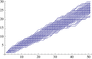
(a) $p=0$

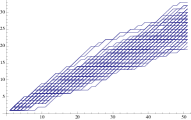
(b) $p=0.4$

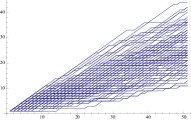
(c) $p=0.8$

(d) $p=1$

Figure 1: Each graph represents a simulation of 100 histories of length 50 for the Pólya–Friedman’s urn (3) (see Example 2.1) with parameter $p\in\{0,\,0.4,\,0.8,\,1\}.$ There is a transition between a Gaussian behavior (Fig.1(a)) and a beta behavior (Fig.1(d)).

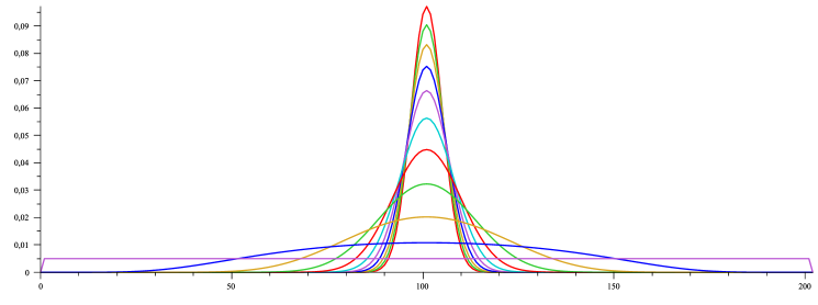
Figure 2: Normalized distribution of the number of black balls after 200 draws ($B_{200}$) for the Pólya–Friedman’s urn (3) with different values of $p\in\{0,\,0.1,\,0.2,\,0.3,\,0.4,\,0.5,\,0.6,\,0.7,\,0.8,\,0.9,\,1\}$. Here, the starting configuration is one black and one white ball. We observe a transition between a Gaussian distribution and a uniform distribution (which is a special case of beta distribution, when $b_{0}=w_{0}=1$).

References

- Andrews (1990) G. Andrews. Euler’s “exemplum memorabile inductionis fallacis” and –trinomial coefficients. Journal of the American Mathematical Society, 3:653–669, 1990.
- Athreya and Karlin (1968) K. B. Athreya and S. Karlin. Embedding of urn schemes into continuous time Markov branching processes and related limit theorems. Annals of Mathematical Statistics, 39:1801–1817, 1968.
- Euler (1801) L. Euler. De evolutione potestatis polynomialis cuiuscunque . Nova Acta Academiae Scientarum Imperialis Petropolitinae, 12:47–57, 1801.
- Flajolet and Sedgewick (2009) P. Flajolet and R. Sedgewick. Analytic Combinatorics. Cambridge University Press, 2009.
- Flajolet et al. (2005) P. Flajolet, J. Gabarró, and H. Pekari. Analytic urns. Annals of Probability, 33:1200–1233, 2005.
- Flajolet et al. (2006) P. Flajolet, P. Dumas, and V. Puyhaubert. Some exactly solvable models of urn process theory. In P. Chassaing, editor, Fourth Colloquium on Mathematics and Computer Science, volume AG of DMTCS Proceedings, pages 59–118, 2006.
- Folland (1995) G. Folland. Introduction to Partial Differential Equations. University Press, Princeton, New Jersey, 1995.
- Freedman (1965) D. A. Freedman. Bernard Friedman’s urn. Annals of Mathematical Statistics, 36:956–970, 1965.
- Hwang et al. (2007) H.-K. Hwang, M. Kuba, and A. Panholzer. Analysis of some exactly solvable diminishing urn models. In Formal Power Series and Algebraic Combinatorics (FPSAC), Tianjin, China, 2007. 12 pages.
- Janson (2004) S. Janson. Functional limit theorems for multitype branching processes and generalized Pólya urns. Stochastic Processes and Applications, 110(2):177–245, 2004.
- Mahmoud (2008) H. M. Mahmoud. Urn Models. Chapman, Orlando, Florida, 2008.
- Morcrette (2012) B. Morcrette. Fully analyzing an algebraic Pólya urn model. In LATIN 2012, volume 7256 of Lecture Notes in Computer Science, pages 568–581, 2012.
- Pólya (1931) G. Pólya. Sur quelques points de la théorie des probabilités. Annales de l’Institut Poincaré, 1:118–161, 1931.
- Smythe (1996) R. T. Smythe. Central limit theorems for urn models. Stochastic Processes and their Applications, 65(1):115–137, 1996.