Coherent quantum ratchets driven by tunnel oscillations: Fluctuations and correlations

Abstract

We study two capacitively coupled double quantum dots focusing on the regime in which one double dot is strongly biased, while no voltage is applied to the other. Then the latter experiences an effective driving force which induces a ratchet current, i.e., a dc current in the absence of a bias voltage. Its current noise is investigated with a quantum master equation in terms of the full-counting statistics. This reveals, that whenever the ratchet current is large, it also exhibits some features of a Poissonian process. By eliminating the drive circuit, we obtain a reduced master equation which provides analytical results for the Fano factor.

I Introduction

The realization of double or triple quantum dots in a linear arrangement GaudreauPRL2006a ; SchroerPRB2007a ; TaubertPRL2008a ; GrangerPRB2010a or in a ring configuration GustavssonPRL2007a ; RoggePRB2008a enables transport experiments in which electrons flow through delocalized orbitals. This delocalization is visible in modified quadruple points of the charging diagram. GaudreauPRL2006a ; SchroerPRB2007a ; TaubertPRL2008a ; GrangerPRB2010a Recently, also the capacitive coupling of two double quantum dots has been achieved. KhrapaiPRL2006a ; PeterssonPRL2009a ; ShinkaiPRL2009a If each double quantum dot is occupied by one electron, the setup represents two interacting charge qubits.PeterssonPRL2009a ; ShinkaiPRL2009a Upon opening one double dot, a current flows and may be used for readout of the other double dot which still forms a charge qubit. GiladPRL2006a ; JiaoPRB2007a ; AshhabPS2009a ; KreisbeckPRB2010a

Opening both double dots enables experiments with two interacting mesoscopic currents. For example, predominantly coherently transported electrons perform tunnel oscillations which act on the other double dot as an effective ac force. This may induce a ratchet or pump effect, i.e., cause a net current in the absence of any bias voltage.StarkEPL2010a A similar ratchet effect has been realized by coupling a double dot to a quantum point contact.KhrapaiPRL2006a This effect is closely related to Coulomb drag MortensenPRL2001a ; SanchezPRL2010a and to using a double quantum dot as noise detector.AguadoPRL2000a ; OnacPRL2006a ; GustavssonPRL2007a In turn, interacting channels may block each other.GattobigioPRB2002a ; BartholdPRL2006a ; SanchezPRB2008a

A common characterization of the current fluctuations in a mesoscopic conductor is the full-counting statistics, LesovikPRL1994a ; BagretsPRB2003a whose cornerstone is a counting variable for the lead electrons. In this way, one obtains a cumulant-generating function for the transported charge. Of particular interest is its variance, because it relates to the zero-frequency limit of the current–current correlation function.MacDonaldRPP1949a Moreover, it indicates whether transport is sub or super Poissonian,BlanterPR2000a even though a more faithful criterion is the $g^{(2)}$ function.EmaryPRB2012a Generally, some further cumulants are specific to the system while beyond a certain order, cumulants exhibit universal features.FlindtPNASUSA2009a

In this work, we explore the noise properties of the ratchet mechanism proposed in Ref. StarkEPL2010a, for capacitively coupled double quantum dots focusing on the full-counting statistics. Besides a numerical study with a master equation for the full ratchet–drive setup, we derive in the spirit of Ref. EmaryPRA2008a, an effective master equation for the ratchet under the influence of the drive circuit. This provides an analytical expression for the cumulant generating function. This approach is beyond a more heuristic elimination of the drive circuitStarkEPL2010a and beyond a golden-rule calculation,AguadoPRL2000a because it includes effects stemming from delocalization and from the broadening of the ratchet levels. Therefore, it holds also for small ratchet detuning.

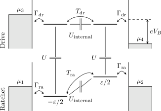
Figure 1: Quantum ratchet (lower circuit, unbiased) capacitively coupled to a drive circuit (top) biased by a voltage $V_{B}$. Each circuit is modeled as two-level system with tunnel couplings $T_{\textrm{ra}}$ and $T_{\textrm{dr}}$, respectively. The ratchet possess a detuning $\varepsilon$, while the drive circuit is undetuned. The dot–lead tunnel rates are $\Gamma_{\textrm{ra}}$ and $\Gamma_{\textrm{dr}}$, while $\mu_{\alpha}$, $\alpha=1,\ldots,4$, denotes the chemical potentials of the leads.

In Sec. II, we introduce our model Hamiltonian for the setup sketched in Fig. 1 and, moreover, introduce a quantum master equation for the full system. Section III is devoted to the elimination of the drive circuit which provides our analytical results. In Sec. IV, we present our numerical results for the higher-order cumulants and test the quality of our approximations.

II Model and method

II.1 Hamiltonian

The four quantum dots and the leads (see Fig. 1) are described by the Hamiltonian $\hat{H}=\hat{H}_{S}+\hat{H}_{B}+\hat{H}_{V}$, where

$$\begin{split}\hat{H}_{S}={}&\sum_{\alpha}\nu_{\alpha}\hat{d}_{\alpha}^{\dagger}\hat{d}_{\alpha}-\big{(}T_{\textrm{ra}}\hat{d}_{1}^{\dagger}\hat{d}_{2}+T_{\textrm{ra}}^{*}\hat{d}_{2}^{\dagger}\hat{d}_{1}\big{)}\\ &-\big{(}T_{\textrm{dr}}\hat{d}_{3}^{\dagger}\hat{d}_{4}+T_{\textrm{dr}}^{*}\hat{d}_{4}^{\dagger}\hat{d}_{3}\big{)}+\sum_{\alpha<\beta}U_{\alpha\beta}\hat{n}_{\alpha}\hat{n}_{\beta}\end{split}$$ (1)

models the quantum dots with the electron creation and annihilation operators $\hat{d}_{\alpha}^{\dagger}$ and $\hat{d}_{\alpha}$. The ratchet circuit ($\alpha=1,2$) has inter-dot tunneling $T_{\textrm{ra}}$ and detuning $\varepsilon$, such that the level splitting becomes

$$\delta=\sqrt{\varepsilon^{2}+4|T_{\textrm{ra}}|^{2}}.$$ (2)

The levels of the drive circuit ($\alpha=3,4$) are not detuned and possess a tunnel matrix element $T_{\textrm{dr}}$. The setup is assumed symmetric, such that inter-channel Coulomb repulsion reads $U\equiv U_{13}=U_{24}$, while the internal repulsions $U_{12}$ and $U_{34}$ are assumed so large, that each channel can be occupied with at most one electron. The inter-channel coupling $U$ by contrast, is relatively weak but nevertheless is the relevant interaction for inducing a ratchet current. StarkEPL2010a We do not take into account more indirect interaction mediated by phonons GrangerNatureP2012a or by a qubit.NietnerPRB2012a

Each dot $\alpha$ is coupled to a lead with chemical potential $\mu_{\alpha}$, where $\mu_{1}=\mu_{2}$, while $\mu_{3}\gg\mu_{4}$, such that all levels of the drive circuit lie within the voltage window. The lead Hamiltonian and the dot-lead couplings read

$$\hat{H}_{B}= \sum_{k\alpha}\varepsilon_{k\alpha}\hat{c}_{k\alpha}^{\dagger}\hat{c}_{k\alpha},$$ (3)

$$\hat{H}_{V}= \sum_{k\alpha}\big{(}V_{k\alpha}\hat{c}_{k\alpha}^{\dagger}\hat{d}_{\alpha}+V_{k\alpha}^{*}\hat{d}_{\alpha}^{\dagger}\hat{c}_{k\alpha}\big{)},$$ (4)

respectively, where $\hat{c}^{\dagger}_{k\alpha}$and $\hat{c}_{k\alpha}$ are the fermionic operators and $\varepsilon_{k\alpha}$ is the corresponding single-particle energy. The system–bath interaction $\hat{H}_{V}$ is determined by the effective tunnel rates $\Gamma_{\alpha}(\varepsilon)=2\pi\sum_{k}|V_{k\alpha}|^{2}\delta(\varepsilon-\varepsilon_{k\alpha})\equiv\Gamma_{\alpha}$, which within the wide-band limit are assumed energy-independent. Throughout this work we use units in which $\hbar=1$.

II.2 Cumulant generating function and master equation

We are interested in the low-frequency properties of the transport process, which can be characterized by the distribution of the number of transported electrons at large times or, equivalently, by the corresponding cumulants. We thus introduce for each lead $\alpha$ a counting variable $\chi_{\alpha}$ such that we obtain the moment generating function $\langle e^{i\bm{\chi}(\hat{\bm{N}}-\bm{N}_{0})}\rangle_{t}\equiv\exp[G(\bm{\chi},t)]$, where $\bm{\chi}=(\chi_{1},\chi_{2},\chi_{3},\chi_{4})$, while $\bm{N}=(N_{1},N_{2},N_{3},N_{4})$ is the electron number in each lead in vector notation with the initial value $\bm{N}_{0}=\langle\hat{\bm{N}}\rangle_{t=0}$. Obviously, the Taylor coefficients of $\exp[G(\bm{\chi},t)]$ are the moments of the lead electron distributions. This allows the definition of occupation cumulants as Taylor coefficients of $\ln\langle e^{i\bm{\chi}(\hat{\bm{N}}-\bm{N}_{0})}\rangle_{t}$. Eventually they grow linearly in time.BagretsPRB2003a Thus, the information about the stationary limit is contained in the time derivative in the long-time limit, so that the (particle) current cumulants of leads 2 and 4 can be written as

$$\kappa_{m,n} =\frac{\partial^{m}}{\partial(i\chi_{2})^{m}}\frac{\partial^{n}}{\partial(i\chi_{4})^{n}}\frac{\partial}{\partial t}G(\bm{\chi},t)\Big{|}_{\bm{\chi}\to 0,t\to\infty}.$$ (5)

Owing to charge conservation, the low-frequency properties of the currents in leads 1 and 3 are identical with those of leads 2 and 4, respectively. Thus, it is sufficient to consider only the latter. The first-order current cumulants are the ratchet current $I_{\textrm{ra}}=e_{0}\kappa_{1,0}$ and the drive current $I_{\textrm{dr}}=e_{0}\kappa_{0,1}$, where $e_{0}$ denotes the elementary charge. The second-order derivatives correspond to the zero-frequency limit of the current-current correlation functions,MacDonaldRPP1949a in particular, $S_{\textrm{ra}}=e_{0}^{2}\kappa_{2,0}$. Since our focus lies on the ratchet current, we introduce the notation $\kappa_{m}\equiv\kappa_{m,0}$.

The cumulant generating function $G(\bm{\chi},t)$ can be obtained from a Markovian master equation approach by unraveling the reduced density operator according to the number of electrons $N_{\alpha}$ in the leads. BagretsPRB2003a Alternatively, one may attribute a counting variable to the system–lead tunnel operators LevitovJMP1996a ; GogolinPRB2006a ; SchallerPRB2009a or multiply the full density operator by $e^{i\bm{\chi}\cdot\hat{\bm{N}}}$ before tracing out the leads.KaiserAP2007a The resulting augmented density operator $\rho(\bm{\chi},t)$ relates to the cumulant generating function via $\ln[\operatorname{tr}\rho(\bm{\chi},t)]=G(\bm{\chi},t)$, while its limit $\rho(\bm{\chi}\to\bm{0},t)$ is the usual reduced density operator. Moreover, $\rho(\bm{\chi},t)$ obeys the master equation

$$\dot{\rho}(\bm{\chi},t) =\mathcal{L}(\bm{\chi})\rho(\bm{\chi},t)$$

$$\equiv\Big{[}\mathcal{L}_{0}+\sum_{\alpha,s=\pm}(e^{si\chi_{\alpha}}-1)\mathcal{J}^{s}_{\alpha}\Big{]}\rho(\bm{\chi},t),$$ (6)

where $\mathcal{L}_{0}$ is the Liouville operator, in our case the one obtained within Bloch-Redfield approximation. For a short derivation, see Appendix A. The superoperator $\mathcal{J}^{+}_{\alpha}$ describes tunneling of an electron from dot $\alpha$ to the respective lead, while $\mathcal{J}^{-}_{\alpha}$ captures the opposite process. Thus, the counting variables keep track of the electron numbers in the leads despite that the latter are traced out. From the master equation (6), one can obtain numerically all cumulants within the recursive scheme of Ref. FlindtPRL2008a, . Before discussing these results, we aim at further analytical progress.

III Elimination of the drive circuit

In order to reduce the number of degrees of freedom, such that an analytically solvable master equation emerges, we eliminate the drive circuit along the lines of Ref. EmaryPRA2008a, . We start by separating the master equation for $\rho(\bm{\chi},t)$, Eq. (6), into contributions for the ratchet, the drive circuit, and their mutual interaction,

$$\dot{\rho}(\chi_{2},t) =\big{[}\mathcal{L}_{\textrm{ra}}(\chi_{2})+\mathcal{L}_{\textrm{dr}}+U\mathcal{L}_{\textrm{ra--dr}}\big{]}\rho(\chi_{2},t).$$ (7)

Since we focus on the ratchet current, we keep only the counting variable $\chi_{2}$ for the right lead of the ratchet circuit. The interaction Liouvillian

$$\mathcal{L}_{\textrm{ra--dr}}\rho=-\frac{i}{2}[\Delta\hat{n}_{\textrm{dr}}\Delta\hat{n}_{\textrm{ra}},\;\rho],$$ (8)

is governed by the occupation imbalances $\Delta\hat{n}_{\textrm{ra}}=\hat{n}_{2}-\hat{n}_{1}$ and $\Delta\hat{n}_{\textrm{dr}}=\hat{n}_{4}-\hat{n}_{3}$, which allow one to approximately write the ratchet–drive interaction Hamiltonian as StarkEPL2010a $U(\hat{n}_{1}\hat{n}_{3}+\hat{n}_{2}\hat{n}_{4})\approx(U/2)\Delta\hat{n}_{\textrm{dr}}\Delta\hat{n}_{\textrm{ra}}$. Thereby we neglect terms that cause global shifts of all dot energies. They are not relevant here, because for all parameters considered below, the onsite energies stay far from the Fermi surfaces.

After transforming master equation (7) into Laplace space, straightforward algebra EmaryPRA2008a provides for the ratchet an effective Liouvillian $\mathcal{L}_{\textrm{eff}}$, which follows from the relation

$$[z-\mathcal{L}_{\textrm{eff}}(\chi_{2},z)]^{-1} \equiv\operatorname{tr}_{\textrm{dr}}\{[z-\mathcal{L}(\chi_{2})]^{-1}\rho_{\textrm{dr}}^{\textrm{stat}}\}$$ (9)

and depends on the stationary state $\rho_{\textrm{dr}}^{\textrm{stat}}$ of the drive circuit. Taylor expansion up to second order in the interaction constant $U$ and subsequent evaluation of the partial trace yields

$$\mathcal{L}_{\textrm{eff}}(\chi_{2},z) =\mathcal{L}_{\textrm{ra}}(\chi_{2})+U\mathcal{L}_{\textrm{eff}}^{(1)}(z)+U^{2}\mathcal{L}_{\textrm{eff}}^{(2)}(z)$$ (10)

with the linear and quadratic corrections

$$\mathcal{L}_{\textrm{eff}}^{(1)}(z)= -\frac{i}{2}\langle\Delta\hat{n}_{\textrm{dr}}\rangle[\Delta\hat{n}_{\textrm{ra}},\;\bullet],$$ (11)

$$\begin{split}\mathcal{L}_{\textrm{eff}}^{(2)}(z)=&-\frac{1}{4}\sum_{m}C(z-\lambda_{\textrm{ra}}^{(m)})\\ &\times[\Delta\hat{n}_{\textrm{ra}},\;\bullet]|\phi_{\textrm{ra}}^{(m)}\rangle\!\rangle\!\langle\!\langle\tilde{\phi}_{\textrm{ra}}^{(m)}|[\Delta\hat{n}_{\textrm{ra}},\;\bullet].\end{split}$$ (12)

Here we employ the superoperator notation of Ref. Carmichael2008a, and define $[M,\bullet]\rho\equiv[M,\rho]$. Moreover, we have introduced the spectral decomposition of the ratchet Liouvillian, $\sum_{m}\lambda_{\textrm{ra}}^{(m)}|\phi_{\textrm{ra}}^{(m)}\rangle\!\rangle\!\langle\!\langle\tilde{\phi}_{\textrm{ra}}^{(m)}|$, with the eigenvalues $\lambda^{(m)}=0,-\Gamma_{\textrm{ra}},-\Gamma_{\textrm{ra}}/2\pm i\delta$, and the left and right eigenvectors $\langle\!\langle\tilde{\phi}_{\textrm{ra}}^{(m)}|$ and $|\phi_{\textrm{ra}}^{(m)}\rangle\!\rangle$, respectively. Here a difficulty arises from the fact that the Liouvillian of a double quantum dot in the zero-bias limit is defective, i.e., it does not possess a complete set of eigenvectors (for details, see Appendix B). Then one may proceed either by constructing a generalized eigenbasis or by introducing a small perturbation that lifts the defectiveness, and finally consider the limit of vanishing perturbation. MolerSIAMReview1978a Since all levels are assumed to stay far from the Fermi surfaces, the impact of the interaction on the jump operators can be neglected safely. Thus, the jump operators $\mathcal{J}_{2}^{\pm}$ of the effective model coincide with the ones of the full Liouvillian.

The dependence on the drive circuit enters via the Laplace transformed auto correlation function of the population imbalance

$$C(t)=\langle\Delta\tilde{n}_{\textrm{dr}}(t)\Delta\tilde{n}_{\textrm{dr}}(0)\rangle-\langle\Delta\hat{n}_{\textrm{dr}}\rangle^{2}$$ (13)

evaluated at the eigenvalues of the ratchet Liouvillian, $C(z-\lambda_{\textrm{ra}}^{(m)})$, which fulfills $C^{*}(z)=C(z^{*})$. For a derivation, see Appendix C. Below we will find that the poles of $C(z)$ are related to the extrema of the ratchet current.

The linear contribution to the effective Liouvillian, $\mathcal{L}_{\textrm{eff}}^{(1)}$ merely provides a small additional bias for the ratchet circuit, but does not induce any non-equilibrium effect. Thus, we omit this term and focus on the impact of $\mathcal{L}_{\textrm{eff}}^{(2)}$. By a straightforward but tedious evaluation of Eq. (12), we obtain in the Fock basis $\{|0\rangle\!\langle 0|,|1\rangle\!\langle 1|,|2\rangle\!\langle 2|,|2\rangle\!\langle 1|,|1\rangle\!\langle 2|\}$ the expression

$$\mathcal{L}_{\textrm{eff}}^{(2)}(z)=\begin{pmatrix}0&0&0&0&0\\ 0&0&0&0&0\\ 0&0&0&0&0\\ 0&0&0&A(z)&B^{*}(z^{*})\\ 0&0&0&B(z)&A^{*}(z^{*})\end{pmatrix},$$ (14)

where the terms

$$A(z)= -\frac{|T|^{2}}{\delta^{2}}\big{[}2C(z+\Gamma_{\textrm{ra}})-\Gamma_{\textrm{ra}}C^{\prime}(z+\Gamma_{\textrm{ra}})\big{]}$$

$$-\sum_{s=\pm}\frac{(\delta+s\varepsilon)^{2}}{4\delta^{2}}C(z+\Gamma_{\textrm{ra}}/2+si\delta),$$ (15)

$$B(z)= \frac{T^{2}}{\delta^{2}}\big{[}2C(z+\Gamma_{\textrm{ra}})-\Gamma_{\textrm{ra}}C^{\prime}(z+\Gamma_{\textrm{ra}})$$

$$-C(z+\Gamma_{\textrm{ra}}/2+i\delta)-C(z+\Gamma_{\textrm{ra}}/2-i\delta)\big{]}$$ (16)

contain a non-Markovian correction through the dependence on the Laplace variable $z$. For the resulting effective ratchet Liouvillian, $\mathcal{L}_{\textrm{ra}}(\chi_{2})+U^{2}\mathcal{L}_{\textrm{eff}}^{(2)}(z)$, the cumulant generating function can be obtained by a standard procedure, namely by computing the eigenvalue that vanishes for $\chi_{2}\to 0$.BagretsPRB2003a This yields a somewhat bulky expression and, thus, we restrict ourselves to the Markovian limit obtained by $z\to 0$. By differentiation with respect to $\chi_{2}$, we obtain the current and the zero-frequency noise as

$$I_{\textrm{ra}}= {}\frac{e_{0}2b\varepsilon}{\delta}\operatorname{Im}\big{[}\big{(}-\Gamma_{\textrm{ra}}/2+i\delta\big{)}C\big{(}\Gamma_{\textrm{ra}}/2+i\delta\big{)}\big{]},$$ (17)

$$S_{\textrm{ra}}= {}\frac{e_{0}^{2}b}{\delta^{2}}\operatorname{Im}\big{[}(-\Gamma_{\textrm{ra}}\varepsilon^{2}+i\delta\varepsilon^{2}+i\delta^{3})C(\Gamma_{\textrm{ra}}/2+i\delta)\big{]},$$ (18)

where $b={4|T_{\textrm{ra}}|^{2}U^{2}}/{\delta(4\delta^{2}+\Gamma_{\textrm{ra}}^{2})}$. These expression, in turn, allow us to simplify the cumulant generating function $G(\chi_{2},t)$. After evaluating the time derivative and the limit $t\to\infty$ contained in definition (5) of the current-cumulant, we obtain the generating function

$$G_{\textrm{eff}}^{(I)}(\chi_{2}) =\frac{i(I_{\textrm{ra}}/e_{0})\sin(\chi_{2})+(S_{\textrm{ra}}/e_{0}^{2})[\cos(\chi_{2})-1]}{1+\frac{b\Gamma_{\textrm{ra}}^{2}}{2\delta U^{2}}[\cos(\chi_{2})-1]},$$ (19)

which within the present approximation contains the full information about the low-frequency properties of the ratchet current. The presence of the counting variable $\chi_{2}$ in the denominator, however, renders the actual calculation of higher-order cumulants a formidable task. Only in the golden-rule limit, i.e., to lowest order in $\Gamma_{\textrm{ra}}$, the denominator becomes independent of $\chi_{2}$, so that $G_{\text{eff}}^{(I)}(\chi_{2})=i(I_{\text{ra}}^{(0)}/e_{0})\sin(\chi_{2})+(S_{\text{ra}}^{(0)}/e_{0}^{2})[\cos(\chi_{2})-1]$. Consequently, we obtain the current cumulants

$$\kappa_{n}=\frac{\partial^{n}}{\partial(i\chi_{2})^{n}}G_{\text{eff}}^{(I)}(\chi_{2})\Big{|}_{\chi_{2}=0}=\begin{cases}I_{\text{ra}}^{(0)}/e_{0}&\text{for odd $n$}\\ S_{\text{ra}}^{(0)}/e_{0}^{2}&\text{for even $n$}\end{cases}$$ (20)

where the upper index $(0)$ refers to the limit $\Gamma_{\textrm{ra}}\to 0$. It turns out to be a good approximation, unless universal cumulant oscillations set in, as we will discuss in Sec. IV.2.

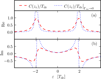
Figure 2: (a) Real and (b) imaginary part of the auto correlation function (dashed lines) of the drive population imbalance in Laplace representation, $C(z_{\varepsilon})$, evaluated at the broadened resonance of the ratchet Liouvillian, $z_{\varepsilon}=\Gamma_{\textrm{ra}}/2+i({\varepsilon^{2}+4|T_{\textrm{ra}}|^{2}})^{1/2}$ with $\Gamma_{\textrm{ra}}=0.5\,T_{\textrm{dr}}$ and $T_{\textrm{ra}}=0.2\,T_{\textrm{dr}}$, as function of the detuning $\varepsilon$. The dotted lines correspond to the limit $\Gamma_{\textrm{ra}}\to 0$. The dot–lead coupling is $\Gamma_{\textrm{dr}}=T_{\textrm{ra}}$.

Before testing the quality of this approximation and the parameter dependence of the results, we close this section by a remark on a formal aspect of the perturbation theory. Both the current (17) and the zero-frequency noise (18) are proportional to the auto correlation function of the population imbalance, $C(z)$, evaluated at the broadened level splitting of the ratchet, where the Laplace variable reads $z_{\varepsilon}=\Gamma_{\textrm{ra}}/2+i(\varepsilon^{2}+4|T_{\textrm{ra}}|^{2})^{1/2}$. Thus we expect the ratchet current to exhibit resonance peaks. Taking into account the broadening distinguishes the present result from that of Ref. StarkEPL2010a, . There the ratchet current has been computed from the golden-rule rates for noise-induced transitions between ratchet eigenstates. While this treatment accounts properly for delocalization effects, it predicts too pronounced resonance peaks. Formally, the golden-rule solution is restored by the replacement $C(\Gamma_{\text{ra}}/2+i\delta)\to C(i\delta)$ in Eq. (17). Figure 2 visualizes that for ratchet detunings close to resonances, the difference between the two approximations may be significant.

IV Characterization of the ratchet current

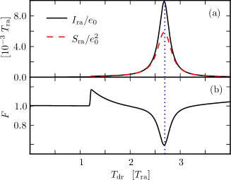
Figure 3: (a) Ratchet current $I_{\textrm{ra}}$, its zero-frequency noise $S_{\textrm{ra}}$, and (b) the resulting Fano factor $F=S_{\textrm{ra}}/e_{0}|I_{\textrm{ra}}|$ as function of the tunnel matrix element of the drive circuit. The results are computed with the full master equation. The other parameters are $\Gamma_{\textrm{ra}}=\Gamma_{\textrm{dr}}=0.1\;T_{\textrm{ra}}$, $U=0.5\;T_{\textrm{ra}}$, and $\varepsilon=5\;T_{\textrm{ra}}$. The vertical dotted line marks the resonance condition $4|T_{\text{dr}}|^{2}=\varepsilon^{2}+4|T_{\textrm{ra}}|^{2}$.

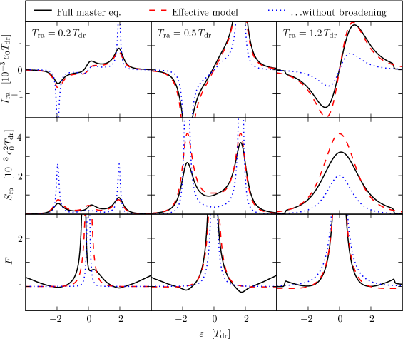
Figure 4: Ratchet current (upper row), zero-frequency noise (middle), and Fano factor (lower row) as function of the ratchet detuning $\varepsilon$ for various tunnel couplings $T_{\textrm{ra}}$. Results for the full master equation (solid lines) are compared to the analytical results (17) and (18) (dashed). Dotted lines mark the golden-rule results which ignore the broadening $\Gamma_{\text{ra}}$. The dot-lead tunneling rates are $\Gamma_{\textrm{ra}}=0.5\,T_{\textrm{dr}}$ and $\Gamma_{\textrm{dr}}=0.2\;T_{\textrm{dr}}$, while the inter-channel coupling reads $U=0.2\,T_{\textrm{dr}}$.

Before starting with the analysis of the ratchet current fluctuations, let us compare the present case to that of a ratchet driven by an ac field. There, the current exhibits resonance peaks with large current and low zero-frequency noise.StrassPRL2005a ; KaiserAP2007a For large driving amplitudes, the same behavior is visible at multi-photon resonances. Figure 3 shows the corresponding result for the present driving by tunnel oscillations. When the level splitting of the ratchet matches the tunnel frequency of the drive circuit, we indeed observe the qualitatively same behavior. Here however, we do not find higher-order resonances and, moreover, the Fano factor does not reach the extremely small values found in Ref. StrassPRL2005a, . The reason for this is that for realistic parameters, the driving via Coulomb interaction with the upper circuit is much weaker than direct ac driving by, e.g., a high-frequency gate voltage.Stehlik2012a The kink in the Fano factor stems from a small step in the current and can be attributed to an energy difference of many-particle states that crosses the Fermi level of the ratchet. StarkEPL2010a This confirms our picture in which the tunnel oscillations of electrons in the drive circuit act like an ac driving with (angular) frequency $\Omega=|2T_{\text{dr}}|$ determined by the tunnel splitting.

IV.1 Zero-frequency noise and Fano factor

If the tunnel coupling of the ratchet is smaller than that of the drive circuit, $T_{\text{ra}}<T_{\text{dr}}$, one can adjust the ratchet bias $\varepsilon$ such, that the resonance condition $\varepsilon^{2}+4|T_{\textrm{ra}}|^{2}=4|T_{\textrm{dr}}|^{2}$ is met. By contrast, for $T_{\text{ra}}>T_{\text{dr}}$ this is not the case. In order to first sketch the global behavior, we first consider the current, the zero-frequency noise, and the resulting Fano factor in dependence of the ratchet bias. We compare numerical results obtained from the full master equation with the analytical solution of Sec. III. Moreover, we also discuss the analytical expressions (17) and (18) to lowest order in $\Gamma_{\text{ra}}$, because this restores the golden-rule results of Ref. StarkEPL2010a, .

Figure 4 provides an overview to the behavior. The current which is depicted in the first row, exhibits the expected resonance peaks provided that $T_{\text{ra}}<T_{\text{dr}}$. If the tunnel matrix element is rather small ($T_{\text{ra}}=0.2\,T_{\text{dr}}$), we witness also the small peaks at small values of $\varepsilon$, which we predicted within our analytical treatment. Upon increasing the inter-dot tunneling $T_{\text{ra}}$, the current peaks naturally increase as well. Once $T_{\text{ra}}>T_{\text{dr}}$, the resonance peaks fade away while the structure at $\varepsilon\approx 0$ becomes rather pronounced. In all regimes, the analytical result (17) for the current is well confirmed. The main difference is the absence of the slight asymmetry with respect to reverting the detuning, $\varepsilon\to-\varepsilon$. Nevertheless, the characteristics of the current as function of $\varepsilon$ is by and large antisymmetric, which implies a current reversal close to zero detuning. In order to capture also the lack of perfect antisymmetry, we would have to consider the linear perturbation $\mathcal{L}_{\text{eff}}^{(1)}$ which, however, would impede concise analytical results. For the parameters used in Fig. (4), the golden-rule expression of Ref. StarkEPL2010a, , i.e., Eq. (17) to lowest order in $\Gamma_{\text{ra}}$, reproduces the behavior only qualitatively. It predicts too sharp peaks, because this approximation does not account for the level broadening of the ratchet. The deviation is quite significant in the non-resonant case $T_{\text{ra}}>T_{\text{dr}}$.

The main features such as the location of the peaks are also found for the zero-frequency noise plotted in the middle row. An important difference is found only close to $\varepsilon=0$, where the current vanishes for symmetry reasons. The noise nevertheless remains finite and may even have a peak. This behavior is reflected by the Fano factor which stays close to the Poissonian value $F=1$ for detunings far from the current reversal point $\varepsilon=0$. There the current vanishes, while the noise remains finite, such that $F$ diverges. The reason for this universal behavior can be understood from the analytical results for the current and the noise. Both $I_{\text{ra}}$ and $S_{\text{ra}}$ depend on the drive circuit via the drive correlation function $C(z)$ which, thus, cancels in their ratio, i.e., in the Fano factor. On a smaller scale, we observe in the Fano factor occasional kinks in less important regions in which the current is rather small. There a small change in the denominator of $F=S_{\text{ra}}/e_{0}|I_{\text{ra}}|$ may have a strong effect.

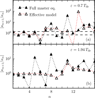
Figure 5: Cumulant ratio $|\kappa_{n+1}/\kappa_{n}|$ versus order $n$ for the parameters used in the second column of Fig. 4 for two values of the detuning $\varepsilon$. The value $\varepsilon\approx 1.94\,T_{\text{dr}}$ corresponds to the resonance between ratchet and drive circuit. The horizontal lines in panel (a) mark the analytical result (20) valid to lowest order in $\Gamma_{\text{ra}}$, i.e., $F$ and $1/F$. The dotted lines serve as guide to the eye.

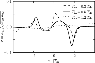
Figure 6: Correlation coefficient $r$ versus detuning $\varepsilon$ for the parameters used in Fig. 4.

IV.2 Higher-order cumulants

For a refined study of the current noise, we investigate also the cumulants of higher order, where we express the results in terms of the ratio between subsequent cumulants, $|\kappa_{n+1}/\kappa_{n}|$. For this quantity, the limit of small $\Gamma_{\text{ra}}$ is rather interesting, because our analytical result (20) implies that the cumulant ratio alternates between the Fano factor and its reciprocal. Such behavior is characteristic for a bi-directional Poisson process.LevitovPRB2004a The usual Poisson process with $|\kappa_{n+1}/\kappa_{n}|=\text{const}$ emerges as special case if the backward current is negligible. The higher-order cumulants of the effective Liouvillian for larger values of $\Gamma_{\text{ra}}$ can be evaluated from the generating function (19), but the expressions become rather bulky, so that one has to resort to a numerical evaluation.

Figure 5 shows a comparison of these two approximations together with the result of the full master equation. For a small ratchet detuning below the resonance [panel(a)], we find that all three solutions agree quite well and that the first few cumulants exhibit the predicted alternation between the values $F$ and $1/F$. For higher orders, the generic universal cumulant oscillations set in,FlindtPNASUSA2009a which obviously is beyond our analytical approach. At the resonance, the universal oscillations start even already at lower order and Eq. (20) no longer holds. This is in agreement with our earlier observation that the broadening of the ratchet levels plays a significant role for resonant driving.

IV.3 Cross correlations

Let us finally consider the cross correlations between the drive current and the ratchet current. They can be characterized by the cumulant $\kappa_{1,1}$, which is equivalent to the covariance of the transported charge in the two circuits. As a dimensionless measure, we introduce the correlation coefficient $r\equiv\kappa_{11}/\sqrt{\kappa_{20}\;\kappa_{02}}$, which is bounded by $-1\leq r\leq 1$. The results depicted in Fig. 6 demonstrate that the correlation between the two currents is rather low. While it can be up to $|r|\sim 0.1$ at the resonances, it is hardly noticeable in the non-resonant case $T_{\textrm{ra}}>T_{\text{dr}}$.

V Conclusions

A double quantum dot with detuned energy levels may act as quantum ratchet or quantum pump when driven out of equilibrium. An external force with zero net bias acting locally upon such system can induce a dc current. Here we investigated a ratchet with a particular driving, namely one that stems from the capacitive coupling to a further double quantum dot which, however, is biased. Electrons flowing through the drive circuit perform tunnel oscillations which indeed induce phenomena similar to those induced by deterministic ac driving. In this work we mainly focused on the fluctuations of the emerging ratchet current. Besides a numerical solution with a master equation for all four quantum dots, we derived an effective ratchet Liouvillian by eliminating the drive circuit. In this way, we obtained analytical results even for higher-order cumulants, which agree well with those of the full master equation provided that the tunnel splitting of the drive circuit is larger than that of the ratchet.

As a common feature of driving by tunnel oscillations and driving by an ac field, we found resonance peaks at which the current assumes a maximum, while the relative noise characterized by the Fano factor is minimal. However, clearly sub-Poissonian noise is only found for large detuning of the ratchet levels. This noise reduction should be measurable, even though it is not as pronounced as in the case of ac driving, mainly because it requires large driving amplitudes which cannot be achieved by capacitive coupling. For less detuned ratchet levels, the Fano factor is typically of the order one, unless the detuning is so small that its orbitals are fully delocalized. Then the lack of sufficiently strong asymmetry keeps the current at a low value, while the zero-frequency noise stays finite. Thus, the Fano factor being the ratio of these two quantities assumes very large values. This generic behavior of the Fano factor is explained by our analytical results which reveal that both the current and the zero-frequency noise are proportional to the correlation function of the drive circuit. Thus the Fano factor depends only on the shape of the ratchet eigenfunctions, while the correlation function cancels.

The higher-order cumulants tend to alternate between two values. This indicates a bi-directional Poisson process and implies that a backward current becomes relevant. With increasing order, however, universal oscillations with ever larger amplitude dominate. The onset of the universal oscillations marks the point at which our analytically obtained higher-order cumulants significantly deviate from those for the full master equation. Nevertheless, the physically relevant cumulants of lower order are well within our analytical treatment.

The more global picture is such that the noise is close to the Poissonian level, whenever the current is relatively large. Thus possible applications and measurements of a ratchet current induced by tunnel oscillations, should not be hindered by current fluctuations.

Appendix A Liouvillian and jump operators

For a system-bath Hamiltonian, one can derive for the reduced system density operator $\rho$ the Bloch-Redfield or Born-Markov master equation Blum1996a ; Carmichael2002a ; Breuer2003a

$$\begin{split}\dot{\rho}(t)=&-i[\hat{H}_{S},\;\rho(t)]\\ &-\int_{0}^{\infty}ds\operatorname{tr}_{B}[\hat{H}_{V},\;[\tilde{H}_{V}(-s),\;\rho(t)R_{0}]]\\ \equiv{}&\mathcal{L}_{0}\rho(t),\end{split}$$ (21)

where $R_{0}$ is the reference density operator of the environment, while $\hat{H}_{V}$ describes the system-bath coupling. It has to be weak, such that coherent system dynamics dominates. Augmenting the environment density operator by a counting variable for the lead electrons according to $\rho(t)R_{0}\to\rho(t)e^{i\bm{\chi}(\hat{\bm{N}}-\bm{N}_{0})}R_{0}$, yields the $\bm{\chi}$-dependent density operator $\rho(\bm{\chi},t)$ whose trace is the moment-generating function introduced in Sec. III.KaiserAP2007a Furthermore, one obtains by inserting the same ansatz into Eq. (21) the master equation (6) upon which all our results are based.

For the evaluation of the time integral in Eq. (21), it is convenient to work in the eigenbasis of the system Hamiltonian, defined by $E_{k}|m\rangle=\hat{H}_{S}|m\rangle$. Then one obtains for the density matrix elements the equation of motion $\dot{\rho}_{mn}(\bm{\chi},t)=\sum_{kl}[\mathcal{L}(\bm{\chi})]_{mn,kl}\;\rho_{kl}(\bm{\chi},t)$, where the decomposed Liouvillian

$$[\mathcal{L}(\bm{\chi})]_{mn,kl}=[\mathcal{L}_{0}]_{mn,kl}+\sum_{\alpha,s=\pm}(e^{si\chi_{\alpha}}-1)[\mathcal{J}^{s}_{\alpha}]_{mn,kl}$$ (22)

consists of the contributions

$$[\mathcal{L}_{0}]_{mn,kl} =-i\delta_{km}\delta_{ln}(E_{m}-E_{n})+\sum_{\alpha,s=\pm}[\mathcal{J}^{s}_{\alpha}]_{mn,kl}$$

$$\hskip 8.61108pt-\frac{1}{2}\delta_{ln}\sum_{\alpha,p}\gamma_{\alpha,pk}[\hat{d}_{\alpha}]_{mp}[\hat{d}_{\alpha}^{\dagger}]_{pk}$$

$$\hskip 8.61108pt-\frac{1}{2}\delta_{km}\sum_{\alpha,p}\gamma_{\alpha,pl}[\hat{d}_{\alpha}]_{lp}[\hat{d}_{\alpha}^{\dagger}]_{pn}$$

$$\hskip 8.61108pt-\frac{1}{2}\delta_{ln}\sum_{\alpha,p}\bar{\gamma}_{\alpha,kp}[\hat{d}_{\alpha}^{\dagger}]_{mp}[\hat{d}_{\alpha}]_{pk}$$

$$\hskip 8.61108pt-\frac{1}{2}\delta_{km}\sum_{\alpha,p}\bar{\gamma}_{\alpha,lp}[\hat{d}_{\alpha}^{\dagger}]_{lp}[\hat{d}_{\alpha}]_{pn},$$ (23)

$$[\mathcal{J}^{-}_{\alpha}]_{mn,kl} =\frac{1}{2}(\gamma_{\alpha,mk}+\gamma_{\alpha,nl})[\hat{d}_{\alpha}^{\dagger}]_{mk}[\hat{d}_{\alpha}]_{ln},$$ (24)

$$[\mathcal{J}^{+}_{\alpha}]_{mn,kl} =\frac{1}{2}(\bar{\gamma}_{\alpha,km}+\bar{\gamma}_{\alpha,ln})[\hat{d}_{\alpha}]_{mk}[\hat{d}_{\alpha}^{\dagger}]_{ln}.$$ (25)

The effective rates

$$\gamma_{\alpha,mn} =\Gamma_{\alpha}f_{\alpha}(E_{m}-E_{n}),$$ (26)

$$\bar{\gamma}_{\alpha,mn} =\Gamma_{\alpha}[1-f_{\alpha}(E_{m}-E_{n})],$$ (27)

depend on the Fermi functions of the leads, $f_{\alpha}(\omega)\equiv f(\omega-\mu_{\alpha})=\{\exp[(\omega-\mu_{\alpha})/k_{B}T]+1\}^{-1}$, while

$$\Gamma_{\alpha} =2\pi\sum_{k}|V_{k\alpha}|^{2}\delta(\omega-\varepsilon_{k\alpha})$$ (28)

denotes the spectral densities of the dot-lead couplings, which within a wide-band limit are assumed energy independent.

Appendix B Spectral decomposition of the ratchet Liouvillian

In the energy basis $\{|0\rangle\!\langle 0|,|e\rangle\!\langle e|,|g\rangle\!\langle g|,|g\rangle\!\langle e|,|e\rangle\!\langle g|\}$ the ratchet Liouvillian for vanishing counting variable $\chi_{2}\to 0$ reads

$$\mathcal{L}_{\textrm{ra}}=\begin{pmatrix}-\Gamma_{\textrm{ra}}&\Gamma_{\textrm{ra}}&0&0&0\\ 0&-\Gamma_{\textrm{ra}}&0&0&0\\ \Gamma_{\textrm{ra}}&0&0&0&0\\ 0&0&0&-\frac{\Gamma_{\textrm{ra}}}{2}+i\delta&0\\ 0&0&0&0&-\frac{\Gamma_{\textrm{ra}}}{2}-i\delta\\ \end{pmatrix}.$$ (29)

Within the perturbative treatment of Sec. III, we need to compute functions $f(\mathcal{L}_{\text{ra}})$ of this matrix, such as the propagator $\exp(\mathcal{L}_{\text{ra}}t)$ or the resolvent $(z-\mathcal{L}_{\text{ra}})^{-1}$, which is usually achieved by spectral decomposition of the Liouvillian. Here however this is hindered by the fact that $\mathcal{L}_{\text{ra}}$ is defective, i.e., it does not possess a complete set of eigenvectors. The problem arises from the upper block

$$L\equiv\begin{pmatrix}-\Gamma_{\textrm{ra}}&\Gamma_{\textrm{ra}}&0\\ 0&-\Gamma_{\textrm{ra}}&0\\ \Gamma_{\textrm{ra}}&0&0\\ \end{pmatrix},$$ (30)

which we transform via

$$S=\begin{pmatrix}0&-1&0\\ 0&0&-{1}/{\Gamma_{\textrm{ra}}}\\ 1&1&{1}/{\Gamma_{\textrm{ra}}}\end{pmatrix},$$ (31)

to the Jordan canonical formGolubSIAMReview1976a ; MolerSIAMReview1978a

$$J=S^{-1}LS=\begin{pmatrix}0&0&0\\ 0&-\Gamma_{\textrm{ra}}&1\\ 0&0&-\Gamma_{\textrm{ra}}\end{pmatrix}.$$ (32)

Its eigenvalues obviously are $0$ and the twofold degenerate $-\Gamma_{\text{ra}}$, and one immediately finds two vectors that obey the eigenvalue equation, namely

$$L|0\rangle={} 0|0\rangle,$$ (33)

$$L|1\rangle={} -\Gamma_{\textrm{ra}}|1\rangle.$$ (34)

A generalized eigenbasis can be found by including a third vector $|2\rangle$ that fulfills GolubSIAMReview1976a ; MolerSIAMReview1978a

$$L|2\rangle=-\Gamma_{\textrm{ra}}|2\rangle+|1\rangle,$$ (35)

i.e., one adds the eigenvector of the degenerate subspace. By repeated multiplication with $L$ follows $L^{k}|2\rangle=(-\Gamma_{\textrm{ra}})^{k}|2\rangle+k(-\Gamma_{\textrm{ra}})^{k-1}|1\rangle$, which implies

$$f(L)|2\rangle =f(\lambda_{2})|2\rangle+f^{\prime}(\lambda_{2})|1\rangle,$$ (36)

where both the function of a matrix and its derivative are defined as the corresponding Taylor series. This relation together with the usual $f(L)|k\rangle=f(\lambda_{k})|k\rangle$ for $k=0,1$, allows us to evaluate any $f(L)$. In particular, we find the propagator

$$e^{Lt}= \begin{pmatrix}e^{-\Gamma_{\textrm{ra}}t}&\Gamma_{\textrm{ra}}te^{-\Gamma_{\textrm{ra}}t}&0\\ 0&e^{-\Gamma_{\textrm{ra}}t}&0\\ 1-e^{-\Gamma_{\textrm{ra}}t}&1-(1+\Gamma_{\textrm{ra}}t)e^{-\Gamma_{\textrm{ra}}t}&1\\ \end{pmatrix},$$ (37)

and the resolvent

$$(z-L)^{-1}= \begin{pmatrix}\frac{1}{z+\Gamma_{\textrm{ra}}}&\frac{\Gamma_{\textrm{ra}}}{(z+\Gamma_{\textrm{ra}})^{2}}&0\\ 0&\frac{1}{z+\Gamma_{\textrm{ra}}}&0\\ \frac{\Gamma_{\textrm{ra}}}{z(z+\Gamma_{\textrm{ra}})}&\frac{\Gamma_{\textrm{ra}}^{2}}{z(z+\Gamma_{\textrm{ra}})^{2}}&\frac{1}{z}\\ \end{pmatrix}.$$ (38)

A poor man’s approach to this procedure MolerSIAMReview1978a is to introduce a small perturbation that lifts the degeneracy of $L$. After evaluating $f(L)$, one considers the limit of vanishing perturbation.

Appendix C Stationary state of the drive circuit

The effective ratchet Liouvillian derived in Sec. III results from a perturbation theory with the stationary states representing the zeroth order. They are determined by the master equationGurvitzPRB1996a

$$\dot{\rho}_{\textrm{dr}} =-i[\hat{H}_{S,\textrm{dr}},\;\rho_{\textrm{dr}}]+\mathcal{D}(\hat{d}_{3}^{\dagger})\rho_{\textrm{dr}}+\mathcal{D}(\hat{d}_{4})\rho_{\textrm{dr}},$$ (39)

with the system Hamiltonian of the drive

$$\hat{H}_{S,\textrm{dr}}=-\big{(}T_{\text{dr}}\hat{d}_{3}^{\dagger}\hat{d}_{4}+T_{\text{dr}}^{*}\hat{d}_{4}^{\dagger}\hat{d}_{3}\big{)}.$$ (40)

The last two terms in the master equation describe dot-lead tunneling, which in the limit of a large voltage bias obeys the Lindblad form

$$\mathcal{D}(\hat{d}_{4})\rho_{\textrm{dr}}=\Gamma_{\textrm{dr}}\;\hat{d}_{4}\rho_{\textrm{dr}}\hat{d}_{4}^{\dagger}-\frac{\Gamma_{\textrm{dr}}}{2}\{\hat{d}_{4}^{\dagger}\hat{d}_{4},\;\rho_{\textrm{dr}}\}.$$ (41)

For the drive circuit, the stationary state can be obtained conveniently after a decomposition of the Liouvillian into the corresponding Fock basis, by which we find

$$\rho_{\textrm{dr}}^{\textrm{stat}}={} \frac{1}{\Gamma_{\textrm{dr}}^{2}+12|T_{\textrm{dr}}|^{2}}$$

$$\times\begin{pmatrix}4|T_{\textrm{dr}}|^{2}&0&0\\ 0&\Gamma_{\textrm{dr}}^{2}+4|T_{\textrm{dr}}|^{2}&-2i\Gamma_{\textrm{dr}}T_{\textrm{dr}}^{*}\\ 0&2i\Gamma_{\textrm{dr}}T_{\textrm{dr}}&4|T_{\textrm{dr}}|^{2}\end{pmatrix}.$$ (42)

The auto correlation function of the population imbalance $\Delta\hat{n}_{\textrm{dr}}=\hat{n}_{4}-\hat{n}_{3}$ in Laplace space is defined as

$$C(z) =\int_{0}^{\infty}dt\;e^{-zt}\big{[}\langle\Delta\tilde{n}_{\textrm{dr}}(t)\Delta\tilde{n}_{\textrm{dr}}(0)\rangle-\langle\Delta\hat{n}_{\textrm{dr}}\rangle^{2}\big{]}$$

$$=\langle\Delta\tilde{n}_{\textrm{dr}}(z)\Delta\hat{n}_{\textrm{dr}}\rangle-\frac{1}{z}\langle\Delta\hat{n}_{\textrm{dr}}\rangle^{2},$$ (43)

with the stationary occupation

$$\langle\Delta\hat{n}_{\textrm{dr}}\rangle =-\frac{\Gamma_{\textrm{dr}}^{2}}{\Gamma_{\textrm{dr}}^{2}+12|T_{\textrm{dr}}|^{2}}$$ (44)

and the corresponding correlation function

$$\langle\Delta\tilde{n}_{\textrm{dr}}(z)\Delta\hat{n}_{\textrm{dr}}\rangle=\frac{1}{z}\frac{2z+\Gamma_{\textrm{dr}}}{\Gamma_{\textrm{dr}}^{2}+12|T_{\textrm{dr}}|^{2}}$$

$$\hskip 10.00002pt\times\frac{\Gamma_{\textrm{dr}}^{2}(z+\Gamma_{\textrm{dr}})^{2}+4z(2z+3\Gamma_{\textrm{dr}})|T_{\textrm{dr}}|^{2}}{(z+\Gamma_{\textrm{dr}})^{2}(2z+\Gamma_{\textrm{dr}})+4(2z+3\Gamma_{\textrm{dr}})|T_{\textrm{dr}}|^{2}}.$$ (45)

References

- (1) L. Gaudreau, S. A. Studenikin, A. S. Sachrajda, P. Zawadzki, A. Kam, J. Lapointe, M. Korkusinski, and P. Hawrylak, Phys. Rev. Lett. 97, 036807 (2006)
- (2) D. Schröer, A. D. Greentree, L. Gaudreau, K. Eberl, L. C. L. Hollenberg, J. P. Kotthaus, and S. Ludwig, Phys. Rev. B 76, 075306 (2007)
- (3) D. Taubert, M. Pioro-Ladrière, D. Schröer, D. Harbusch, A. S. Sachrajda, and S. Ludwig, Phys. Rev. Lett. 100, 176805 (2008)
- (4) G. Granger, L. Gaudreau, A. Kam, M. Pioro-Ladrière, S. A. Studenikin, Z. R. Wasilewski, P. Zawadzki, and A. S. Sachrajda, Phys. Rev. B 82, 075304 (2010)
- (5) S. Gustavsson, M. Studer, R. Leturcq, T. Ihn, K. Ensslin, D. C. Driscoll, and A. C. Gossard, Phys. Rev. Lett. 99, 206804 (2007)
- (6) M. C. Rogge and R. J. Haug, Phys. Rev. B 77, 193306 (2008)
- (7) V. S. Khrapai, S. Ludwig, J. P. Kotthaus, H. P. Tranitz, and W. Wegscheider, Phys. Rev. Lett. 97, 176803 (2006)
- (8) K. D. Petersson, C. G. Smith, D. Anderson, P. Atkinson, G. A. C. Jones, and D. A. Ritchie, Phys. Rev. Lett. 103, 016805 (2009)
- (9) G. Shinkai, T. Hayashi, T. Ota, and T. Fujisawa, Phys. Rev. Lett. 103, 056802 (2009)
- (10) T. Gilad and S. A. Gurvitz, Phys. Rev. Lett. 97, 116806 (2006)
- (11) H. J. Jiao, X.-Q. Li, and J. Y. Luo, Phys. Rev. B 75, 155333 (2007)
- (12) S. Ashhab, J. Q. You, and F. Nori, Phys. Scr. T137, 014005 (2009)
- (13) C. Kreisbeck, F. J. Kaiser, and S. Kohler, Phys. Rev. B 81, 125404 (2010)
- (14) M. Stark and S. Kohler, EPL 91, 20007 (2010)
- (15) N. A. Mortensen, K. Flensberg, and A.-P. Jauho, Phys. Rev. Lett. 86, 1841 (2001)
- (16) R. Sánchez, R. López, D. Sánchez, and M. Büttiker, Phys. Rev. Lett. 104, 076801 (2010)
- (17) R. Aguado and L. P. Kouwenhoven, Phys. Rev. Lett. 84, 1986 (2000)
- (18) E. Onac, F. Balestro, L. H. W. van Beveren, U. Hartmann, Y. V. Nazarov, and L. P. Kouwenhoven, Phys. Rev. Lett. 96, 176601 (2006)
- (19) M. Gattobigio, G. Iannaccone, and M. Macucci, Phys. Rev. B 65, 115337 (2002)
- (20) P. Barthold, F. Hohls, N. Maire, K. Pierz, and R. J. Haug, Phys. Rev. Lett. 96, 246804 (2006)
- (21) R. Sánchez, S. Kohler, P. Hänggi, and G. Platero, Phys. Rev. B 77, 035409 (2008)
- (22) G. B. Lesovik and L. S. Levitov, Phys. Rev. Lett. 72, 538 (1994)
- (23) D. A. Bagrets and Yu. V. Nazarov, Phys. Rev. B 67, 085316 (2003)
- (24) D. K. C. MacDonald, Rep. Prog. Phys. 12, 56 (1949)
- (25) Ya. M. Blanter and M. Büttiker, Phys. Rep. 336, 1 (2000)
- (26) C. Emary, C. Pöltl, A. Carmele, J. Kabuss, A. Knorr, and T. Brandes, Phys. Rev. B 85, 165417 (2012)
- (27) C. Flindt, C. Fricke, F. Hohls, T. Novotný, K. Netočný, T. Brandes, and R. J. Haug, Proc. Natl. Acad. Sci. USA 106, 10116 (2009)
- (28) C. Emary, Phys. Rev. A 78, 032105 (2008)
- (29) G. Granger, D. Taubert, C. E. Young, L. Gaudreau, A. Kam, S. A. Studenikin, P. Zawadzki, D. Harbusch, D. Schuh, W.Wegscheider, Z. R.Wasilewski, A. A. Clerk, S. Ludwig, , and A. S. Sachrajda, Nature Phys. 8, 522 (2012)
- (30) C. Nietner, G. Schaller, C. Pöltl, and T. Brandes, Phys. Rev. B 85, 245431 (2012)
- (31) L. S. Levitov, H. W. Lee, and G. B. Lesovik, J. Math. Phys. 37, 4845 (1996)
- (32) A. O. Gogolin and A. Komnik, Phys. Rev. B 73, 195301 (2006)
- (33) G. Schaller, G. Kießlich, and T. Brandes, Phys. Rev. B 80, 245107 (2009)
- (34) F. J. Kaiser and S. Kohler, Ann. Phys. (Leipzig) 16, 702 (2007)
- (35) C. Flindt, T. Novotný, A. Braggio, M. Sassetti, and A.-P. Jauho, Phys. Rev. Lett. 100, 150601 (2008)
- (36) H. J. Carmichael, Statistical Methods in Quantum Optics 2 (Springer–Verlag, 2008)
- (37) C. Moler and C. V. Loan, SIAM Rev. 20, 801 (1978)
- (38) M. Strass, P. Hänggi, and S. Kohler, Phys. Rev. Lett. 95, 130601 (2005)
- (39) J. Stehlik, Y. Dovzhenko, J. R. Petta, J. R. Johansson, F. Nori, H. Lu, and A. C. Gossard, arXiv:1205.6173 [cond-mat]
- (40) L. S. Levitov and M. Reznikov, Phys. Rev. B 70, 115305 (2004)
- (41) K. Blum, Density Matrix Theory and Applications, 2nd ed. (Springer, New York, 1996)
- (42) H. J. Carmichael, Statistical Methods in Quantum Optics 1 (Springer–Verlag, 2002)
- (43) H.-P. Breuer and F. Petruccione, Theory of open quantum systems (Oxford University Press, Oxford, 2003)
- (44) G. H. Golub and J. H. Wilkinson, SIAM Rev. 18, 578 (1976)
- (45) S. A. Gurvitz and Y. S. Prager, Phys. Rev. B 53, 15932 (1996)