Clustering function: a measure of social influence


Mindaugas Bloznelis111Faculty of Mathematics and Informatics, Vilnius University, 03225 Vilnius, Lithuania222Corresponding author mindaugas.bloznelis@mif.vu.lt and Valentas Kurauskas1


Abstract

A commonly used characteristic of statistical dependence of adjacency relations in real networks, the clustering coefficient, evaluates chances that two neighbours of a given vertex are adjacent. An extension is obtained by considering conditional probabilities that two randomly chosen vertices are adjacent given that they have rπ‘Ÿr common neighbours. We denote such probabilities c​l​(r)π‘π‘™π‘Ÿcl(r) and call rβ†’c​l​(r)β†’π‘Ÿπ‘π‘™π‘Ÿr\to cl(r) the clustering function. We compare clustering functions of several networks having non-negligible clustering coefficient. They show similar patterns and surprising regularity. We establish a first order asymptotic (as the number of vertices nβ†’+βˆžβ†’π‘›n\to+\infty) of the clustering function of related random intersection graph models admitting nonvanishing clustering coefficient and asymptotic degree distribution having a finite second moment.

key words: clustering coefficient, social network, intersection graph, power law


2000 Mathematics Subject Classifications: 91D30, 05C80, 05C07, 91C20


1 Introduction

Our study is motivated by the following question: given two vertices of a network, the presence of how many common neighbours would imply with certainty that these two vertices are adjacent. A ”softer” question is about the probability that two vertices with (at least) rπ‘Ÿr common neighbours establish a link. The answer is given by the clustering functions (1) and (2).

Let 𝒒=(𝒱,β„°)𝒒𝒱ℰ{\cal G}=({\cal V},{\cal E}) be a finite graph on vertex set 𝒱𝒱{\cal V} and with edge set β„°β„°{\cal E}. The number of neighbours of a vertex v𝑣v is denoted d​(v)𝑑𝑣d(v). The number of common neighbours of vertices visubscript𝑣𝑖v_{i} and vjsubscript𝑣𝑗v_{j} is denoted d​(vi,vj)𝑑subscript𝑣𝑖subscript𝑣𝑗d(v_{i},v_{j}). We are interested in the fraction of adjacent pairs vi∼vjsimilar-tosubscript𝑣𝑖subscript𝑣𝑗v_{i}\sim v_{j} among all pairs {vi,vj}βŠ‚π’±subscript𝑣𝑖subscript𝑣𝑗𝒱\{v_{i},v_{j}\}\subset{\cal V} having (at least) rπ‘Ÿr common neighbours. Here and below β€™βˆΌsimilar-to\sim’ denotes the adjacency relation of 𝒒𝒒{\cal G}. More formally, let us consider the random pair of distinct vertices {v1βˆ—,v2βˆ—}superscriptsubscript𝑣1superscriptsubscript𝑣2\{v_{1}^{*},v_{2}^{*}\} drawn from 𝒱𝒱{\cal V} uniformly at random. Define the clustering functions of 𝒒𝒒{\cal G}

rβ†’c​l𝒒​(r):=𝐏​(v1βˆ—βˆΌv2βˆ—|d​(v1βˆ—,v2βˆ—)=r),β†’π‘Ÿπ‘subscriptπ‘™π’’π‘Ÿassign𝐏similar-tosuperscriptsubscript𝑣1conditionalsuperscriptsubscript𝑣2𝑑superscriptsubscript𝑣1superscriptsubscript𝑣2π‘Ÿ\displaystyle r\to cl_{\cal G}(r):={\bf{P}}(v_{1}^{*}\sim v_{2}^{*}|\,d(v_{1}^{*},v_{2}^{*})=r), (1)
rβ†’C​l𝒒​(r):=𝐏​(v1βˆ—βˆΌv2βˆ—|d​(v1βˆ—,v2βˆ—)β‰₯r).β†’π‘ŸπΆsubscriptπ‘™π’’π‘Ÿassign𝐏similar-tosuperscriptsubscript𝑣1conditionalsuperscriptsubscript𝑣2𝑑superscriptsubscript𝑣1superscriptsubscript𝑣2π‘Ÿ\displaystyle r\to Cl_{\cal G}(r):={\bf{P}}(v_{1}^{*}\sim v_{2}^{*}|\,d(v_{1}^{*},v_{2}^{*})\geq r). (2)

In the case of a social network (1), (2) could be interpreted as measures of social influence or pressure exercised by the neighbours on a pair of actors to establish a communication link. We remark that characteristics (1) and (2) are related to the clustering coefficient of 𝒒𝒒{\cal G}. We recall its definition for convenience. Let (v1βˆ—,v2βˆ—,v3βˆ—)superscriptsubscript𝑣1superscriptsubscript𝑣2superscriptsubscript𝑣3(v_{1}^{*},v_{2}^{*},v_{3}^{*}) be an ordered triple of distinct vertices drawn from 𝒱𝒱{\cal V} uniformly at random. The conditional probability that v1βˆ—superscriptsubscript𝑣1v_{1}^{*} is adjacent to v2βˆ—superscriptsubscript𝑣2v_{2}^{*}, given that v1βˆ—superscriptsubscript𝑣1v_{1}^{*} and v2βˆ—superscriptsubscript𝑣2v_{2}^{*} are both adjacent to v3βˆ—superscriptsubscript𝑣3v_{3}^{*}, is called the (global) clustering coefficient ([3], [18], [19], [26]). We denote it C=C𝒒=𝐏(v1βˆ—βˆΌv2βˆ—|v1βˆ—βˆΌv3βˆ—,v2βˆ—βˆΌv3βˆ—)C=C_{\cal G}={\bf{P}}(v_{1}^{*}\sim v_{2}^{*}|v_{1}^{*}\sim v_{3}^{*},v_{2}^{*}\sim v_{3}^{*}).

In this paper we study clustering functions first by considering empirical data and then by a rigorous analysis of related random graph models.

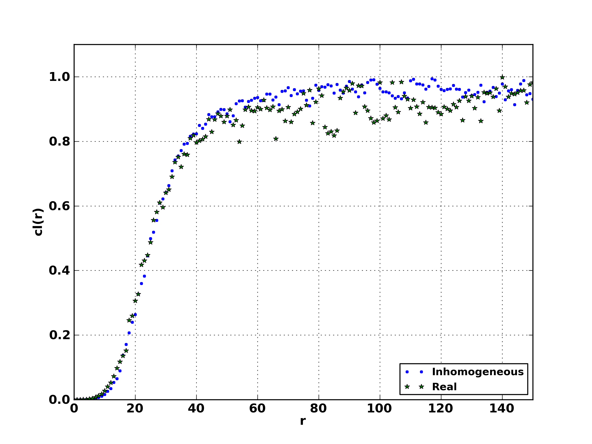
We consider clustering function (1) of real networks admitting positive clustering coefficient: the actor network, where two actors are declared adjacent whenever they have acted in the same film ([29]), and the Facebook network ([1], [14], [27]). We remark that empirical plots show similar pattern and surprising regularity.

Our choice of the random graph model is motivated by an observation of Newman et al. [20] that the clustering property of some social networks (so called affiliation networks) could be explained by the presence of a bipartite graph structure. For example, the bipartite graph, where actors are linked to films, defines the actor network. It seems reasonable that a bipartite graph structure might also be helpful in explaining (at least to some extent) the adjacency relations of Facebook network: two members become adjacent because they share some common interests/attributes.

We secondly consider clustering function (1) of a random intersection graph, where vertices (actors) are prescribed attribute sets independently at random and two vertices are declared adjacent whenever they share at least one common attribute ([17], [15], see also [2], [16]). Random intersection graphs are relatively simple objects and for them rigorous mathematical results can be obtained. We evaluate the probabilities 𝐏​(v1βˆ—βˆΌv2βˆ—|d​(v1βˆ—,v2βˆ—)=r)𝐏similar-tosuperscriptsubscript𝑣1conditionalsuperscriptsubscript𝑣2𝑑superscriptsubscript𝑣1superscriptsubscript𝑣2π‘Ÿ{\bf{P}}(v_{1}^{*}\sim v_{2}^{*}|\,d(v_{1}^{*},v_{2}^{*})=r), r=0,1,2,β€¦π‘Ÿ012…r=0,1,2,\dots for a random intersection graph in Sect. 3 below.

2 Clustering functions: empirical results

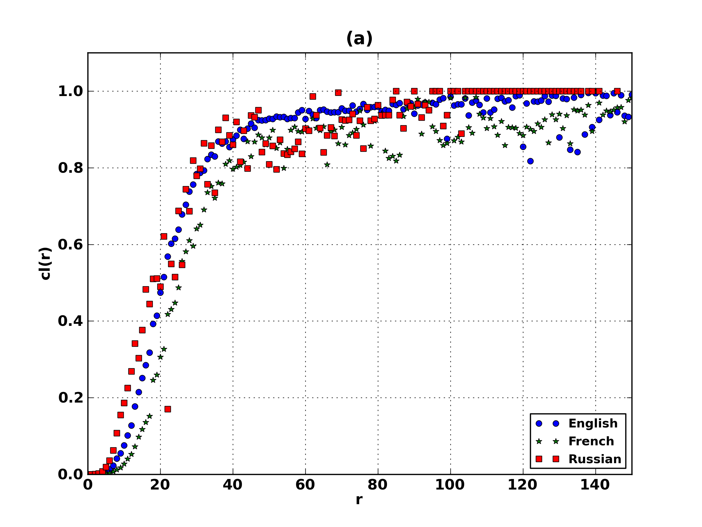
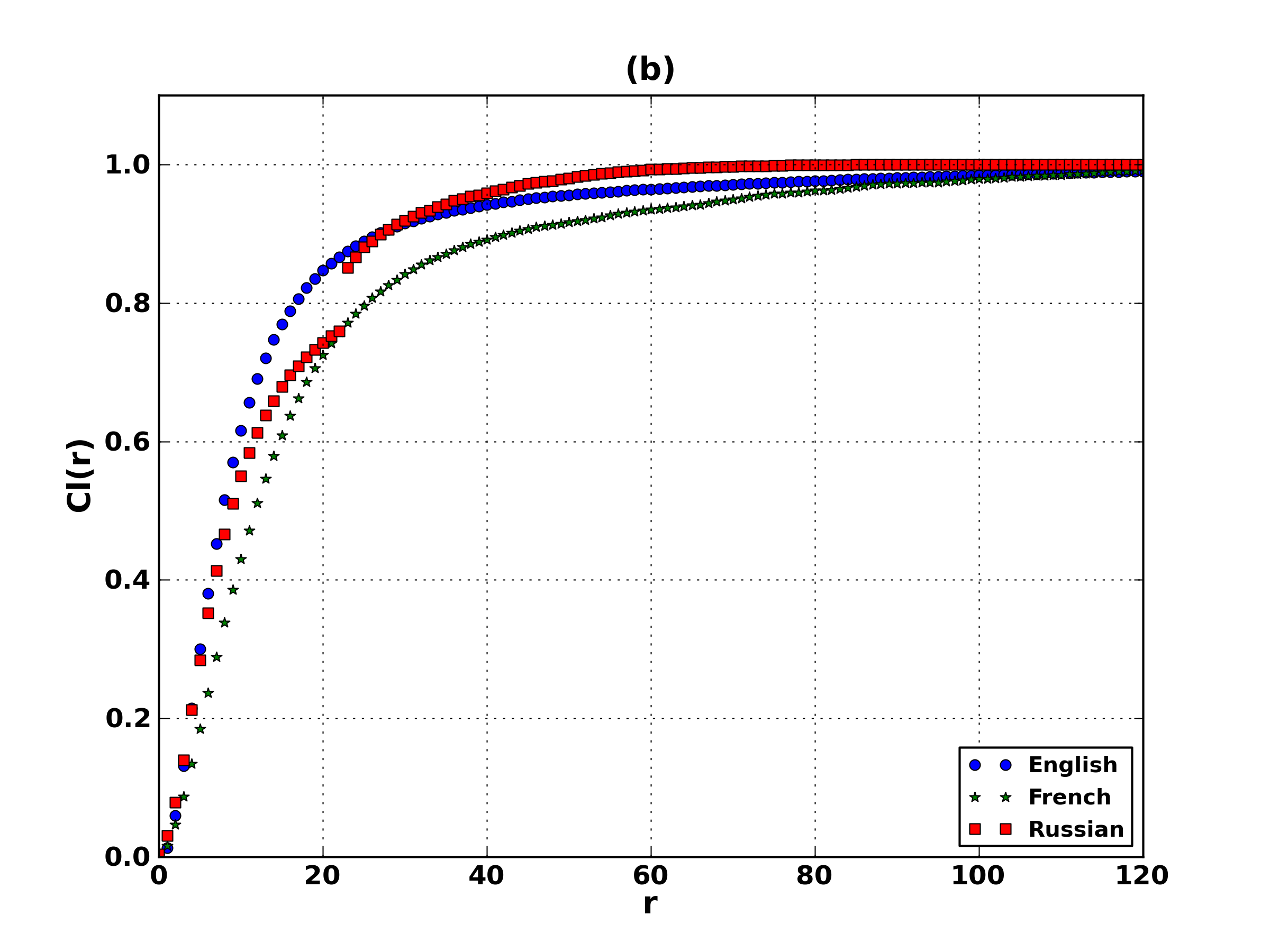
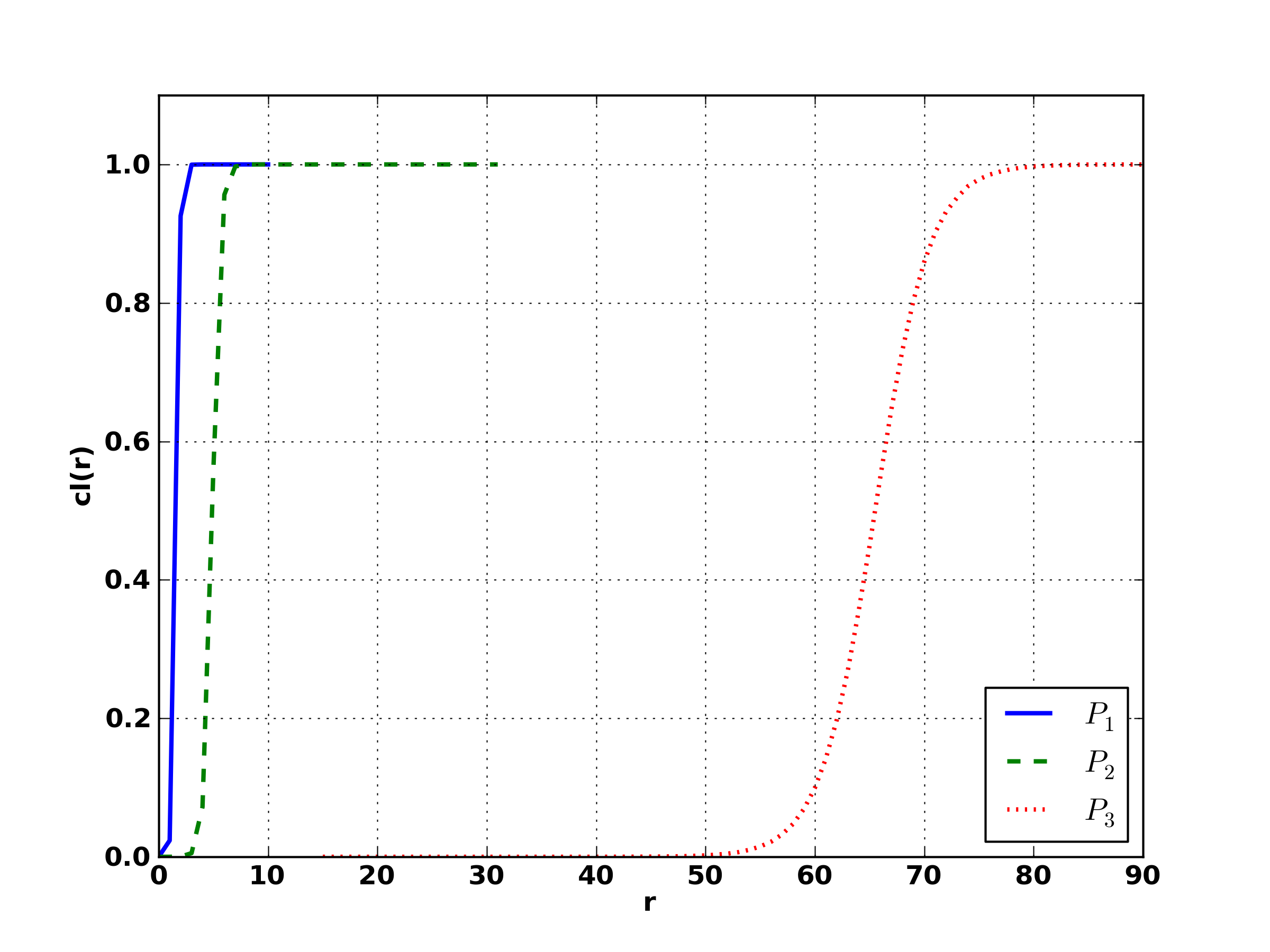
In Figure 1 we plot clustering functions (1) and (2) of three drama actor networks: the English actor network with n=402622𝑛402622n=402622 actors, m=66127π‘š66127m=66127 films and the clustering coefficient C=0.32𝐢0.32C=0.32 (the clustering coefficients here and below are rounded up to 2 decimal places), the French actor network with n=43204𝑛43204n=43204 actors, m=5629π‘š5629m=5629 films and the clustering coefficient C=0.30𝐢0.30C=0.30 and the Russian actor network with n=9880𝑛9880n=9880 actors, m=2459π‘š2459m=2459 films and C=0.44𝐢0.44C=0.44. The data has been obtained from [29].

Refer to caption
Refer to caption
Figure 1: Clustering functions for three actor networks: (a) c​l​(r)π‘π‘™π‘Ÿcl(r), (b) C​l​(r)πΆπ‘™π‘ŸCl(r).

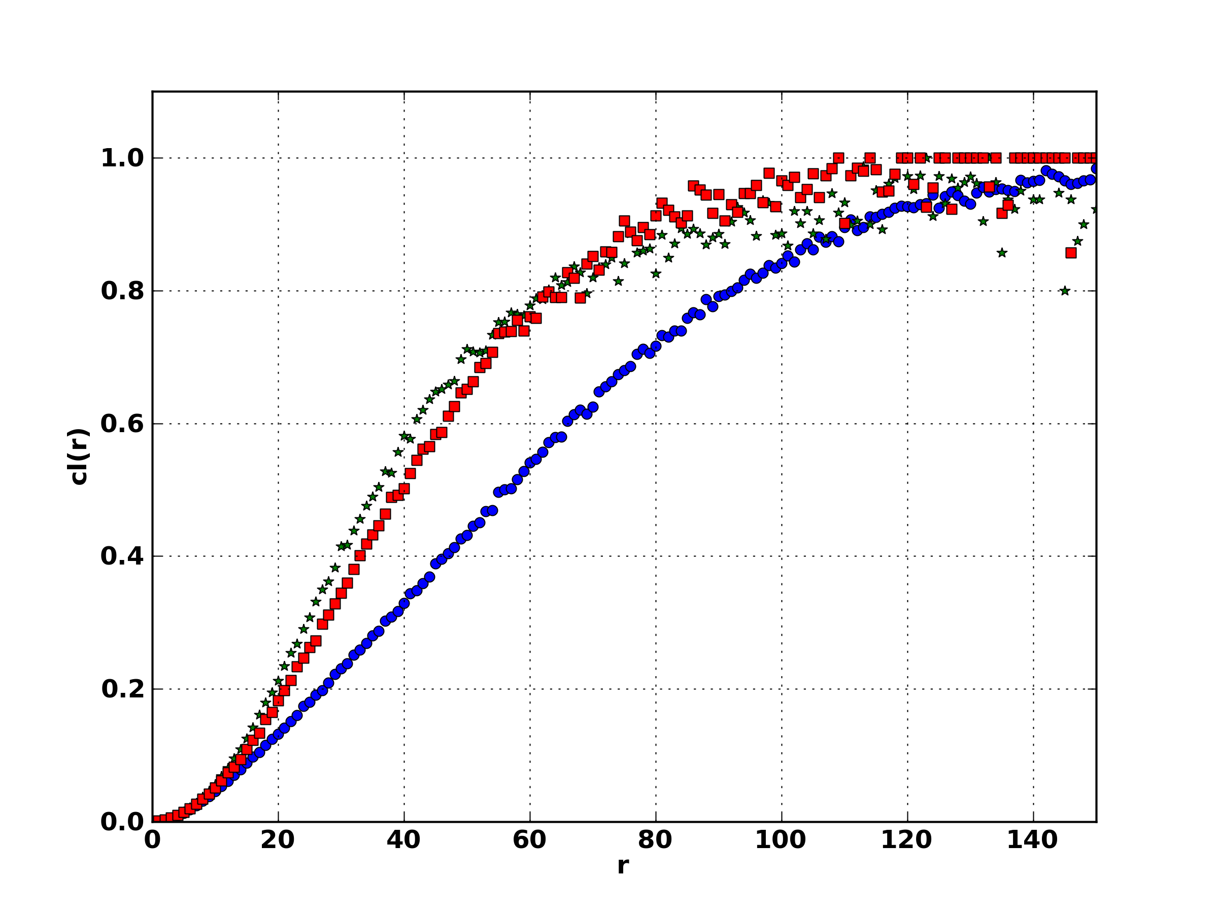
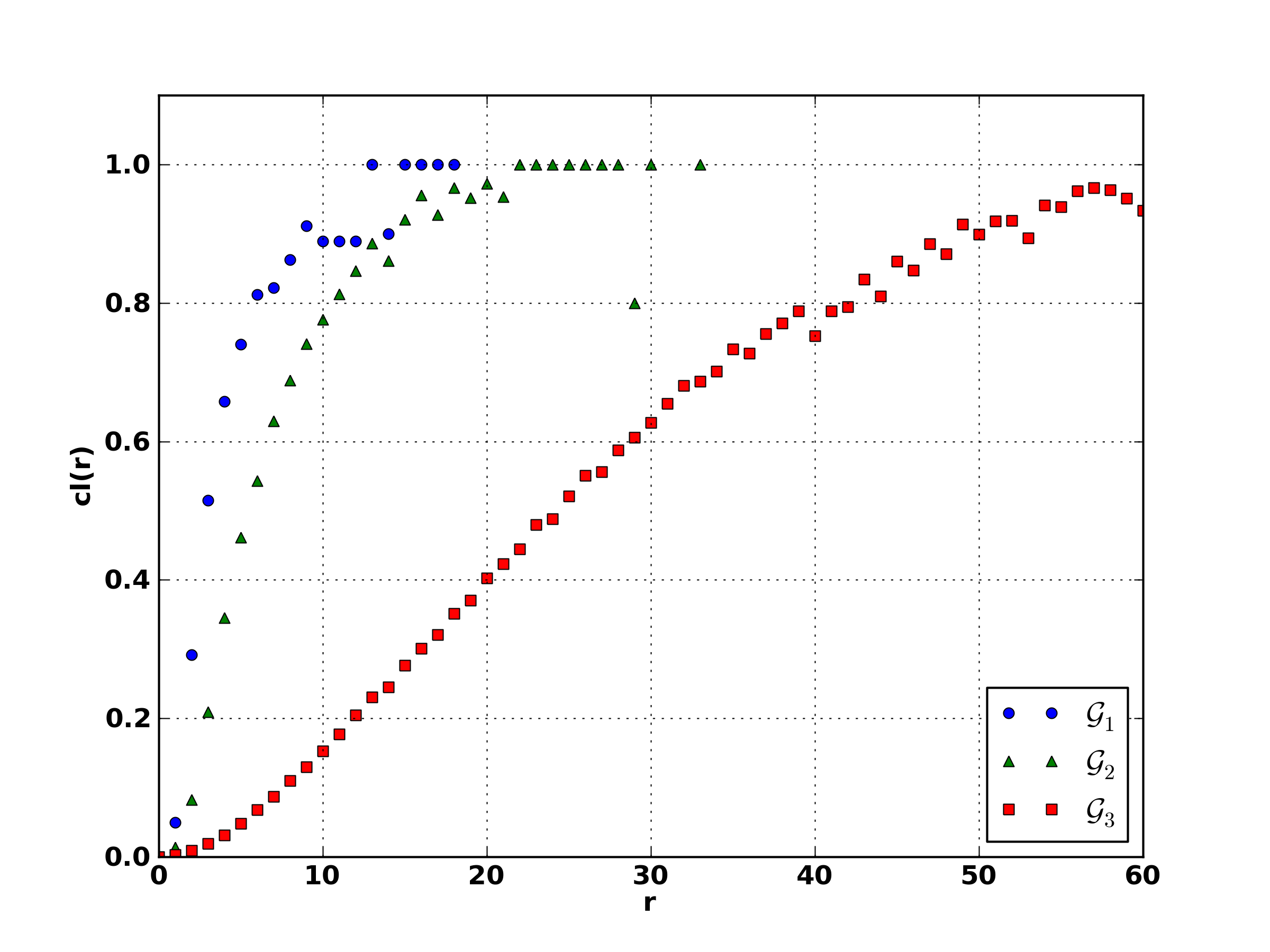
In Figure 2 we plot clustering function (1) of three networks describing relations between community members at three different universities (data from [27]): the first network has n=17425𝑛17425n=17425 vertices and the clustering coefficient C=0.16𝐢0.16C=0.16 (βˆ™βˆ™\bullet blue graph); the second network has n=9414𝑛9414n=9414 vertices and the clustering coefficient C=0.15𝐢0.15C=0.15 (⋆⋆\star green graph); the third network has n=6596𝑛6596n=6596 vertices and the clustering coefficient C=0.16𝐢0.16C=0.16 (β– β– \blacksquare red graph).

Refer to caption
Figure 2: Clustering functions of three university networks.

3 Clustering functions of random intersection graphs

Vertices v1,…,vnsubscript𝑣1…subscript𝑣𝑛v_{1},\dots,v_{n} of an intersection graph are represented by subsets D1,…,Dnsubscript𝐷1…subscript𝐷𝑛D_{1},\dots,D_{n} of a given ground set W={w1,…,wm}π‘Šsubscript𝑀1…subscriptπ‘€π‘šW=\{w_{1},\dots,w_{m}\}. Elements of Wπ‘ŠW are called attributes or keys. Vertices visubscript𝑣𝑖v_{i} and vjsubscript𝑣𝑗v_{j} are declared adjacent if Di∩Djβ‰ βˆ…subscript𝐷𝑖subscript𝐷𝑗D_{i}\cap D_{j}\not=\emptyset. The adjacency relations of such an intersection graph resemble those of some real networks, e.g., the collaboration network, where authors are declared adjacent whenever they have co-authored a paper, or the actor network, where two actors are linked by an edge whenever they have acted in the same film. Random intersection graphs have attracted considerable attention in the recent literature, see, e.g., [4], [5], [7] [10], [13], [22], [21], [28]. They admit a power law degree distribution and tunable clustering. We consider two models of random intesection graphs: the active graph and the inhomogeneous graph.

Active graph. In the active random intersection graph G1​(n,m,P)subscript𝐺1π‘›π‘šπ‘ƒG_{1}(n,m,P) every vertex vi∈V={v1,…,vn}subscript𝑣𝑖𝑉subscript𝑣1…subscript𝑣𝑛v_{i}\in V=\{v_{1},\dots,v_{n}\} selects its attribute set Disubscript𝐷𝑖D_{i} independently at random ([15], [17]). We assume for simplicity that independent random sets D1,…,Dnsubscript𝐷1…subscript𝐷𝑛D_{1},\dots,D_{n} have the same probability distribution

𝐏​(Di=A)=(m|A|)βˆ’1​P​(|A|),Β for Β Β  anyAβŠ‚W.formulae-sequence𝐏subscript𝐷𝑖𝐴superscriptbinomialπ‘šπ΄1𝑃𝐴 for Β Β  anyπ΄π‘Š{\bf{P}}(D_{i}=A)={\tbinom{m}{|A|}}^{-1}P(|A|),\qquad{\text{ for \ \ any}}\quad A\subset W. (3)

In particular, all attributes have equal probabilities to be selected. Here P𝑃P is the common probability distribution of the sizes of selected sets Xi:=|Di|assignsubscript𝑋𝑖subscript𝐷𝑖X_{i}:=|D_{i}| (for each i=1,…,n𝑖1…𝑛i=1,\dots,n we have 𝐏​(Xi=k)=P​(k)𝐏subscriptπ‘‹π‘–π‘˜π‘ƒπ‘˜{\bf{P}}(X_{i}=k)=P(k), k=0,1,…​mπ‘˜01β€¦π‘šk=0,1,\dots m). We remark that X1,…,Xnsubscript𝑋1…subscript𝑋𝑛X_{1},\dots,X_{n} are independent random variables taking values in {0,1,…,m}01β€¦π‘š\{0,1,\dots,m\}.

We study the clustering function

rβ†’c​l​(r)=𝐏​(v1βˆ—βˆΌv2βˆ—|d​(v1βˆ—,v2βˆ—)=r)=𝐏​(v1∼v2|d​(v1,v2)=r)β†’π‘Ÿπ‘π‘™π‘Ÿπsimilar-tosuperscriptsubscript𝑣1conditionalsuperscriptsubscript𝑣2𝑑superscriptsubscript𝑣1superscriptsubscript𝑣2π‘Ÿπsimilar-tosubscript𝑣1conditionalsubscript𝑣2𝑑subscript𝑣1subscript𝑣2π‘Ÿ\displaystyle r\to cl(r)=\,{\bf{P}}(v_{1}^{*}\sim v_{2}^{*}|\,d(v_{1}^{*},v_{2}^{*})=r)\,={\bf{P}}(v_{1}\sim v_{2}|\,d(v_{1},v_{2})=r) (4)

of a sparse random intersection graph with large number of vertices. We remark, that the second identity of (4) follows from the fact that the probability distribution of G1​(n,m,P)subscript𝐺1π‘›π‘šπ‘ƒG_{1}(n,m,P) is invariant under permutation of its vertices. By sparse we mean that the number of edges scales as the number of vertices n𝑛n as nβ†’+βˆžβ†’π‘›n\to+\infty. It is convenient to consider a sequence of random intersection graphs {G(n)}nsubscriptsubscript𝐺𝑛𝑛\{G_{(n)}\}_{n}, where G(n)=G1​(n,m,P)subscript𝐺𝑛subscript𝐺1π‘›π‘šπ‘ƒG_{(n)}=G_{1}(n,m,P) and where m=mnπ‘šsubscriptπ‘šπ‘›m=m_{n} and P=Pn𝑃subscript𝑃𝑛P=P_{n} both depend on n𝑛n. We remark that {G(n)}nsubscriptsubscript𝐺𝑛𝑛\{G_{(n)}\}_{n} is a sequence of sparse random graphs whenever the size X1subscript𝑋1X_{1} of the typical random set is of order (m/n)1/2superscriptπ‘šπ‘›12(m/n)^{1/2} as m,nβ†’βˆžβ†’π‘šπ‘›m,n\to\infty ([6]). Furthermore, assuming that

(i) X1​n/msubscript𝑋1π‘›π‘šX_{1}\sqrt{n/m} converges in distribution to some random variable Z𝑍Z;

(ii) 𝐄​Z<βˆžπ„π‘{\bf{E}}Z<\infty and 𝐄​X1​n/m𝐄subscript𝑋1π‘›π‘š{\bf{E}}X_{1}\sqrt{n/m} converges to 𝐄​Z𝐄𝑍{\bf{E}}Z

one obtains the asymptotic degree distribution of {G(n)}subscript𝐺𝑛\{G_{(n)}\}

limnβ†’+βˆžπβ€‹(d​(v1)=k)=𝐄​eβˆ’Z​𝐄​Z​(Z​𝐄​Z)k/k!,fork=0,1,…,formulae-sequencesubscript→𝑛𝐏𝑑subscript𝑣1π‘˜π„superscript𝑒𝑍𝐄𝑍superscriptπ‘π„π‘π‘˜π‘˜forπ‘˜01…\lim_{n\to+\infty}{\bf{P}}(d(v_{1})=k)={\bf{E}}e^{-Z\,{\bf{E}}Z}(Z\,{\bf{E}}Z)^{k}/k!,\qquad{\text{for}}\qquad k=0,1,\dots, (5)

see [6], [7], [11], [24]. Here d​(v)𝑑𝑣d(v) denotes the degree of a vertex v𝑣v. We remark that a heavy tailed distribution of Z𝑍Z yields a heavy tailed asymptotic degree distribution (5). Along with the first moment condition (ii) we shall also consider the rβˆ’limit-fromπ‘Ÿr-th moment condition

(ii-r) 𝐄​Zr<βˆžπ„superscriptπ‘π‘Ÿ{\bf{E}}Z^{r}<\infty and 𝐄​(X1​n/m)r𝐄superscriptsubscript𝑋1π‘›π‘šπ‘Ÿ{\bf{E}}(X_{1}\sqrt{n/m})^{r} converges to 𝐄​Zr𝐄superscriptπ‘π‘Ÿ{\bf{E}}Z^{r}.

We denote zr=𝐄​Zrsubscriptπ‘§π‘Ÿπ„superscriptπ‘π‘Ÿz_{r}={\bf{E}}Z^{r} and Ξ΄r=𝐄​dβˆ—rsubscriptπ›Ώπ‘Ÿπ„superscriptsubscriptπ‘‘π‘Ÿ\delta_{r}={\bf{E}}d_{*}^{r} where dβˆ—subscript𝑑d_{*} is a random variable with the asymptotic degree distribution 𝐏​(dβˆ—=k)=𝐄​eβˆ’z1​Z​(z1​Z)k/k!𝐏subscriptπ‘‘π‘˜π„superscript𝑒subscript𝑧1𝑍superscriptsubscript𝑧1π‘π‘˜π‘˜{\bf{P}}(d_{*}=k)={\bf{E}}e^{-z_{1}Z}(z_{1}Z)^{k}/k!, k=0,1,β€¦π‘˜01…k=0,1,\dots. We assume below that 𝐄​Z>0𝐄𝑍0{\bf{E}}Z>0, i.e., that the asymptotic degree distribution is non-degenerate. Furthermore, we assume for convenience that the ratio Ξ²n=m/nsubscriptπ›½π‘›π‘šπ‘›\beta_{n}=m/n tends to some β∈(0,+∞]𝛽0\beta\in(0,+\infty] as nβ†’+βˆžβ†’π‘›n\to+\infty.

An important property of the active random intersection graph is that the adjacency relations are statistically dependent events. In particular, the clustering coefficient

α=α(G(n))=𝐏(v1∼v2|v1∼v3,v2∼v3)\alpha=\alpha(G_{(n)})={\bf{P}}(v_{1}\sim v_{2}|v_{1}\sim v_{3},v_{2}\sim v_{3})

of a sparse random intersection graph G(n)subscript𝐺𝑛G_{(n)} is bounded away from zero as nβ†’+βˆžβ†’π‘›n\to+\infty provided that the second moment of the degree distribution is finite and Ξ²<βˆžπ›½\beta<\infty ([7], [11]). In this case we have (see ([7], [11])

Ξ±=Ξ²βˆ’1/2​δ13/2​(Ξ΄2βˆ’Ξ΄1)βˆ’1+o​(1)asnβ†’+∞.formulae-sequence𝛼superscript𝛽12superscriptsubscript𝛿132superscriptsubscript𝛿2subscript𝛿11π‘œ1as→𝑛\displaystyle\alpha=\beta^{-1/2}\delta_{1}^{3/2}(\delta_{2}-\delta_{1})^{-1}+o(1)\qquad{\text{as}}\qquad n\to+\infty. (6)

We remark that for Ξ²=+βˆžπ›½\beta=+\infty we have Ξ±=o​(1)π›Όπ‘œ1\alpha=o(1). For comparison, the (unconditional) edge probability pe:=𝐏​(v1∼v2)assignsubscript𝑝𝑒𝐏similar-tosubscript𝑣1subscript𝑣2p_{e}:={\bf{P}}(v_{1}\sim v_{2}) satisfies for any β∈(0,+∞]𝛽0\beta\in(0,+\infty], see, e.g., [7],

pe=Ξ΄1​nβˆ’1+o​(nβˆ’1)=O​(nβˆ’1).subscript𝑝𝑒subscript𝛿1superscript𝑛1π‘œsuperscript𝑛1𝑂superscript𝑛1p_{e}=\delta_{1}n^{-1}+o(n^{-1})=O(n^{-1}).

Theorems 1 and 2 show a first order asymptotics of the conditional probabilities c​l​(r)π‘π‘™π‘Ÿcl(r) as nβ†’+βˆžβ†’π‘›n\to+\infty in the cases where Ξ²<βˆžπ›½\beta<\infty and Ξ²=βˆžπ›½\beta=\infty, respectively.

Theorem 1.

Let m,nβ†’βˆžβ†’π‘šπ‘›m,n\to\infty. Assume that (i), (ii-2) hold and 𝐄​Z>0𝐄𝑍0{\bf{E}}Z>0. Suppose that Ξ²nβ†’Ξ²βˆˆ(0,+∞)β†’subscript𝛽𝑛𝛽0\beta_{n}\to\beta\in(0,+\infty). Denote Ξ›=Ξ΄1/Ξ²Ξ›subscript𝛿1𝛽\Lambda=\sqrt{\delta_{1}/\beta}. We have

c​l​(r)={pe​eβˆ’Ξ›β€‹(1+o​(1)),r=0;Ξ±Ξ±+(1βˆ’Ξ±)​eΛ​(1+o​(1)),r=1;1βˆ’o​(1),rβ‰₯2.π‘π‘™π‘Ÿcasessubscript𝑝𝑒superscript𝑒Λ1π‘œ1π‘Ÿ0otherwise𝛼𝛼1𝛼superscript𝑒Λ1π‘œ1π‘Ÿ1otherwise1π‘œ1π‘Ÿ2otherwisecl(r)=\begin{cases}p_{e}e^{-\Lambda}(1+o(1)),\qquad\ \ \ \quad r=0;\\ \frac{\alpha}{\alpha+(1-\alpha)e^{\Lambda}}(1+o(1)),\quad\quad\ r=1;\\ 1-o(1),\qquad\qquad\quad\quad\quad\ r\geq 2.\end{cases} (7)

Empirical results of simulated random intersection graphs show that the convergence to the β€œlimiting shapeβ€œ in (7) is rather slow, see Figures 3 and 4 below.

Theorem 2.

Let m,nβ†’βˆžβ†’π‘šπ‘›m,n\to\infty. Assume that (i), (ii-2) hold and 𝐄​Z>0𝐄𝑍0{\bf{E}}Z>0. Suppose that Ξ²nβ†’+βˆžβ†’subscript𝛽𝑛\beta_{n}\to+\infty. We have

c​l​(r)={pe​(1+o​(1)),r=0;Ξ²nβˆ’1/2​(z1/z2)​(1+o​(1))+O​(nβˆ’1),r=1.π‘π‘™π‘Ÿcasessubscript𝑝𝑒1π‘œ1π‘Ÿ0otherwisesuperscriptsubscript𝛽𝑛12subscript𝑧1subscript𝑧21π‘œ1𝑂superscript𝑛1π‘Ÿ1otherwisecl(r)=\begin{cases}p_{e}(1+o(1)),\qquad\ \qquad\qquad\qquad\qquad\ \ r=0;\\ \beta_{n}^{-1/2}(z_{1}/z_{2})(1+o(1))+O(n^{-1}),\quad\quad\ r=1.\end{cases} (8)

In particular, c​l​(0)=O​(nβˆ’1)𝑐𝑙0𝑂superscript𝑛1cl(0)=O(n^{-1}) and c​l​(1)=o​(1)𝑐𝑙1π‘œ1cl(1)=o(1). Furthermore, we have

c​l​(2)={1+o​(1),forΞ²n/nβ†’0;11+Ξ²βˆ—β€‹(Ξ΄2βˆ’Ξ΄1)4​δ1βˆ’6+o​(1),forΞ²n/nβ†’Ξ²βˆ—βˆˆ(0,+∞);o​(1),forΞ²n/nβ†’+∞.𝑐𝑙2casesβ†’1π‘œ1forsubscript𝛽𝑛𝑛0otherwiseβ†’11subscript𝛽superscriptsubscript𝛿2subscript𝛿14superscriptsubscript𝛿16π‘œ1forsubscript𝛽𝑛𝑛subscript𝛽0otherwiseβ†’π‘œ1forsubscript𝛽𝑛𝑛otherwisecl(2)=\begin{cases}1+o(1),\qquad\qquad\qquad\qquad{\text{for}}\qquad\beta_{n}/n\to 0;\\ \frac{1}{1+\beta_{*}(\delta_{2}-\delta_{1})^{4}\delta_{1}^{-6}}+o(1),\qquad\ {\text{for}}\qquad\beta_{n}/n\to\beta_{*}\in(0,+\infty);\\ o(1),\qquad\qquad\qquad\qquad\quad\ \ {\text{for}}\qquad\beta_{n}/n\to+\infty.\end{cases} (9)

Assuming, in addition, that Ξ²nk=o​(n)superscriptsubscriptπ›½π‘›π‘˜π‘œπ‘›\beta_{n}^{k}=o(n) for each k=1,2,3β€‹β€¦π‘˜123italic-…k=1,2,3\dots, we obtain

c​l​(r)=1+o​(1),forr=2,3,….formulae-sequenceπ‘π‘™π‘Ÿ1π‘œ1forπ‘Ÿ23…cl(r)=1+o(1),\qquad{\text{for}}\qquad r=2,3,\dots. (10)

We conclude from (7), (8) that edge dependence measures c​l​(1)𝑐𝑙1cl(1) and α𝛼\alpha are closely related. In particular, we have c​l​(1)=1βˆ’o​(1)⇔α=1βˆ’o​(1)⇔𝑐𝑙11π‘œ1𝛼1π‘œ1cl(1)=1-o(1)\Leftrightarrow\alpha=1-o(1) and c​l​(1)=o​(1)⇔α=o​(1)⇔𝑐𝑙1π‘œ1π›Όπ‘œ1cl(1)=o(1)\Leftrightarrow\alpha=o(1). Furthermore, (9) tells us that the characteristic c​l​(2)𝑐𝑙2cl(2) is able to distinguish between the cases Ξ²n=o​(n)subscriptπ›½π‘›π‘œπ‘›\beta_{n}=o(n) and n=o​(Ξ²n)π‘›π‘œsubscript𝛽𝑛n=o(\beta_{n}). Finally, (10) tells us that any c​l​(r)π‘π‘™π‘Ÿcl(r), r=1,2,β€¦π‘Ÿ12…r=1,2,\dots can’t distinguish between sequences {Ξ²n}subscript𝛽𝑛\{\beta_{n}\} and {Ξ²nβ€²}superscriptsubscript𝛽𝑛′\{\beta_{n}^{\prime}\} growing slower that any power of n𝑛n (take Ξ²n=ln⁑nsubscript𝛽𝑛𝑛\beta_{n}=\ln n and Ξ²nβ€²=ln2⁑nsuperscriptsubscript𝛽𝑛′superscript2𝑛\beta_{n}^{\prime}=\ln^{2}n, for example).

Remark 1. It is likely that (9) can be extended to an arbitrary rπ‘Ÿr as follows

c​l​(r)={1+o​(1),forΞ²n/n4βˆ’2​rβˆ’1β†’0;c​(r,Ξ²βˆ—)+o​(1),forΞ²n/n4βˆ’2​rβˆ’1β†’Ξ²βˆ—βˆˆ(0,+∞);o​(1),forΞ²n/n4βˆ’2​rβˆ’1β†’+∞.π‘π‘™π‘Ÿcasesβ†’1π‘œ1forsubscript𝛽𝑛superscript𝑛42superscriptπ‘Ÿ10otherwiseβ†’π‘π‘Ÿsubscriptπ›½π‘œ1forsubscript𝛽𝑛superscript𝑛42superscriptπ‘Ÿ1subscript𝛽0otherwiseβ†’π‘œ1forsubscript𝛽𝑛superscript𝑛42superscriptπ‘Ÿ1otherwisecl(r)=\begin{cases}1+o(1),\qquad\qquad\quad\,{\text{for}}\qquad\beta_{n}/n^{4-2r^{-1}}\to 0;\\ c(r,\beta_{*})+o(1),\qquad\ \,{\text{for}}\qquad\beta_{n}/n^{4-2r^{-1}}\to\beta_{*}\in(0,+\infty);\\ o(1),\qquad\quad\qquad\quad\ \ \,{\text{for}}\qquad\beta_{n}/n^{4-2r^{-1}}\to+\infty.\end{cases}

Here c​(r,Ξ²βˆ—)=(Ξ²βˆ—r/2​z1βˆ’rβˆ’2​z2r​zr2+1)βˆ’1π‘π‘Ÿsubscript𝛽superscriptsuperscriptsubscriptπ›½π‘Ÿ2superscriptsubscript𝑧1π‘Ÿ2superscriptsubscript𝑧2π‘Ÿsuperscriptsubscriptπ‘§π‘Ÿ211c(r,\beta_{*})=(\beta_{*}^{r/2}z_{1}^{-r-2}z_{2}^{r}z_{r}^{2}+1)^{-1}. We note that numbers zi=𝐄​Zisubscript𝑧𝑖𝐄superscript𝑍𝑖z_{i}={\bf{E}}Z^{i} can be expressed in terms of moments of the asymptotic degree distribution (5).

Proofs of Theorems 1 and 2 are given in Sect. 5.

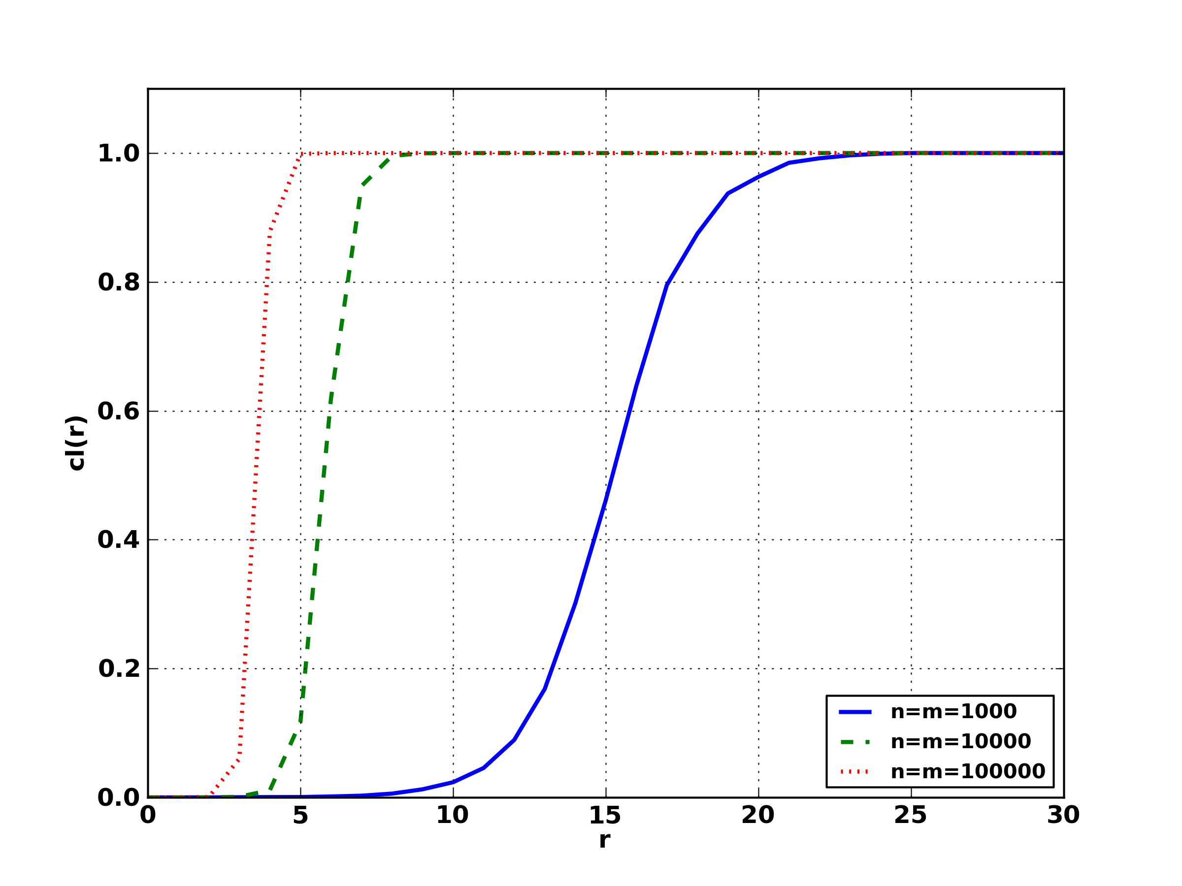
Fig. 3 illustrates the convergence to a step function shown by Theorem 1. Here we plot clustering function (1) of simulated random intersection graphs Gi=G​(ni,mi,P)subscript𝐺𝑖𝐺subscript𝑛𝑖subscriptπ‘šπ‘–π‘ƒG_{i}=G(n_{i},m_{i},P), where ni=mi=102+isubscript𝑛𝑖subscriptπ‘šπ‘–superscript102𝑖n_{i}=m_{i}=10^{2+i}, i=1,2,3𝑖123i=1,2,3, and P​(10)=1𝑃101P(10)=1.

In Fig. 4 we plot (1) for simulated random intersection graphs Gi=G​(n,m,Pi)subscriptπΊπ‘–πΊπ‘›π‘šsubscript𝑃𝑖G_{i}=G(n,m,P_{i}), where n=m=104π‘›π‘šsuperscript104n=m=10^{4} and Pi​(3i)=1subscript𝑃𝑖superscript3𝑖1P_{i}(3^{i})=1, i=1,2,3𝑖123i=1,2,3. Fig. 4 illustrates the influence of the size of random sets.

Refer to caption
Figure 3: Convergence to the step function for random intersection graphs with all sets of size 10.
Refer to caption
Figure 4: Clustering function of random intersection graphs with n=m=10000π‘›π‘š10000n=m=10000 and Pi​(3i)=1subscript𝑃𝑖superscript3𝑖1P_{i}(3^{i})=1, i=1,2,3𝑖123i=1,2,3.

Inhomogeneous graph. The inhomogeneous random intersection graph G1​(n,m,P1,P2)subscript𝐺1π‘›π‘šsubscript𝑃1subscript𝑃2G_{1}(n,m,P_{1},P_{2}) on the vertex set V={v1,…,vn}𝑉subscript𝑣1…subscript𝑣𝑛V=\{v_{1},\dots,v_{n}\} is obtained as follows. We first generate independent random variables A1,…,An,B1,…,Bmsubscript𝐴1…subscript𝐴𝑛subscript𝐡1…subscriptπ΅π‘šA_{1},\dots,A_{n},B_{1},\dots,B_{m} such that each Aisubscript𝐴𝑖A_{i} has the probability distribution P1subscript𝑃1P_{1} and each Bjsubscript𝐡𝑗B_{j} has the probability distribution P2subscript𝑃2P_{2}. Then, conditionally on the realized values {Ai,Bj}i,j=1n,msuperscriptsubscriptsubscript𝐴𝑖subscript𝐡𝑗𝑖𝑗1π‘›π‘š\{A_{i},B_{j}\}_{i,j=1}^{n,m}, we include the attribute wj∈Wsubscriptπ‘€π‘—π‘Šw_{j}\in W in the set Disubscript𝐷𝑖D_{i} with probability pi​j=min⁑{1,Ai​Bj​(n​m)βˆ’1/2}subscript𝑝𝑖𝑗1subscript𝐴𝑖subscript𝐡𝑗superscriptπ‘›π‘š12p_{ij}=\min\{1,A_{i}B_{j}(nm)^{-1/2}\} independently for each i𝑖i and j𝑗j (see [2], [8], [9], [23]). Our motivation of studying this random graph model is that its clustering function approximates empirical data remarkably well, see Figure 8 below.

We consider a sequence of inhomogeneous intersection graphs {G~n=G1​(n,m,P1,P2)}subscript~𝐺𝑛subscript𝐺1π‘›π‘šsubscript𝑃1subscript𝑃2\{{\tilde{G}}_{n}=G_{1}(n,m,P_{1},P_{2})\}, where P1subscript𝑃1P_{1}, P2subscript𝑃2P_{2} remain fixed while m=mnπ‘šsubscriptπ‘šπ‘›m=m_{n} and n𝑛n tend to infinity. We denote ak=𝐄​A1ksubscriptπ‘Žπ‘˜π„superscriptsubscript𝐴1π‘˜a_{k}={\bf{E}}A_{1}^{k} and bk=𝐄​B1ksubscriptπ‘π‘˜π„superscriptsubscript𝐡1π‘˜b_{k}={\bf{E}}B_{1}^{k}. A simple calculation shows (see Section 5 below) that the edge probability pe=𝐏​(v1∼v2)subscript𝑝𝑒𝐏similar-tosubscript𝑣1subscript𝑣2p_{e}={\bf{P}}(v_{1}\sim v_{2}) of G1​(n,m,P1,P2)subscript𝐺1π‘›π‘šsubscript𝑃1subscript𝑃2G_{1}(n,m,P_{1},P_{2}) satisfies

pe=a12​b2​nβˆ’1+o​(nβˆ’1).subscript𝑝𝑒superscriptsubscriptπ‘Ž12subscript𝑏2superscript𝑛1π‘œsuperscript𝑛1p_{e}=a_{1}^{2}b_{2}n^{-1}+o(n^{-1}). (11)

Hence, {G~n}subscript~𝐺𝑛\{{\tilde{G}}_{n}\} is a sequence of sparse graphs. We remark that this sequence admits a power law asymptotic degree distribution [8].

In Theorem 3 below we show a first order asymptotics of the clustering function c​l​(β‹…)𝑐𝑙⋅cl(\cdot) in the case where the ratio Ξ²n=m/nsubscriptπ›½π‘›π‘šπ‘›\beta_{n}=m/n has a non-zero finite limit. In addition, we show that G~nsubscript~𝐺𝑛{\tilde{G}}_{n} admits a nonvanishing clustering coefficient Ξ±=Ξ±(G~n)=𝐏(v1∼v2|v1∼v3,v2∼v3)\alpha=\alpha({\tilde{G}}_{n})={\bf{P}}(v_{1}\sim v_{2}|v_{1}\sim v_{3},v_{2}\sim v_{3}).

Theorem 3.

Let m,nβ†’βˆžβ†’π‘šπ‘›m,n\to\infty. Assume that 0<𝐄​A12<∞0𝐄superscriptsubscript𝐴120<{\bf{E}}A_{1}^{2}<\infty and 0<𝐄​B13<∞0𝐄superscriptsubscript𝐡130<{\bf{E}}B_{1}^{3}<\infty. Suppose that Ξ²nβ†’Ξ²βˆˆ(0,+∞)β†’subscript𝛽𝑛𝛽0\beta_{n}\to\beta\in(0,+\infty). Then we have

Ξ±=b3​κb3​κ+Ξ²+o​(1)𝛼subscript𝑏3πœ…subscript𝑏3πœ…π›½π‘œ1\alpha=\frac{b_{3}\kappa}{b_{3}\kappa+\sqrt{\beta}}+o(1)\qquad\qquad\qquad\qquad\ \ (12)

and

c​l​(r)={a12​b2βˆ—β€‹nβˆ’1​(1+o​(1)),r=0;b3βˆ—β€‹ΞΊb3βˆ—β€‹ΞΊ+β​(1+o​(1)),r=1;1βˆ’o​(1),rβ‰₯2.π‘π‘™π‘Ÿcasessuperscriptsubscriptπ‘Ž12subscriptsuperscript𝑏2superscript𝑛11π‘œ1π‘Ÿ0otherwisesubscriptsuperscript𝑏3πœ…subscriptsuperscript𝑏3πœ…π›½1π‘œ1π‘Ÿ1otherwise1π‘œ1π‘Ÿ2otherwisecl(r)=\begin{cases}a_{1}^{2}b^{*}_{2}n^{-1}(1+o(1)),\qquad\quad\ \ r=0;\\ \frac{b^{*}_{3}\kappa}{b^{*}_{3}\kappa+\sqrt{\beta}}(1+o(1)),\qquad\qquad r=1;\\ 1-o(1),\qquad\qquad\quad\quad\quad\ \ \ r\geq 2.\end{cases} (13)

Here ΞΊ=a1​a2βˆ’1​b2βˆ’2πœ…subscriptπ‘Ž1superscriptsubscriptπ‘Ž21superscriptsubscript𝑏22\kappa=a_{1}a_{2}^{-1}b_{2}^{-2} and Β bkβˆ—=𝐄​B1k​eβˆ’a1​B1/Ξ²subscriptsuperscriptπ‘π‘˜π„superscriptsubscript𝐡1π‘˜superscript𝑒subscriptπ‘Ž1subscript𝐡1𝛽b^{*}_{k}={\bf{E}}B_{1}^{k}e^{-a_{1}B_{1}/\sqrt{\beta}}.

The proof of Theorem 3 is given in Sect. 5.

4 Discussion

The first order asymptotics (7), (9), (10) and (13) suggests that the clustering function c​l​(β‹…)𝑐𝑙⋅cl(\cdot) of a large intersection graph with a square integrable asymptotic degree distribution can be approximated by a step - like function. Furthermore, c​l​(1)𝑐𝑙1cl(1) is closely related to the clustering coefficient.

Simulations in Figures 3 and 4 show that the convergence in (7) can be rather slow and we observe a sigmoid function approximation of the step function. Furthermore, the larger is the average degree, the more remote is the β€œstepβ€œ from the origin and the more gradual is the slope of the clustering function.

Clustering functions of real networks considered in Figures 1 and 3 have even more gradual slope, a phenomena perhaps related to the inhomogeneity of the degree sequence. We remark that the actor network and the Facebook are considered as having power law degree sequences which do not admit a finite (theoretical) second moment, see, e.g., [12], [14]. In order to learn more about the influence of the inhomogeneity of the degree sequence on the slope of the clustering function rβ†’c​l​(r)β†’π‘Ÿπ‘π‘™π‘Ÿr\to cl(r) we select various subnetworks of real networks according to certain regularity conditions satisfied by their degree sequences. We observe that the inhomogeneity (heavy tail) of the degree sequence affects the slope of the clustering function: the heavier the tail the more gradual is the slope of the clustering function. We illustrate these observations in Figures 5 and 6.

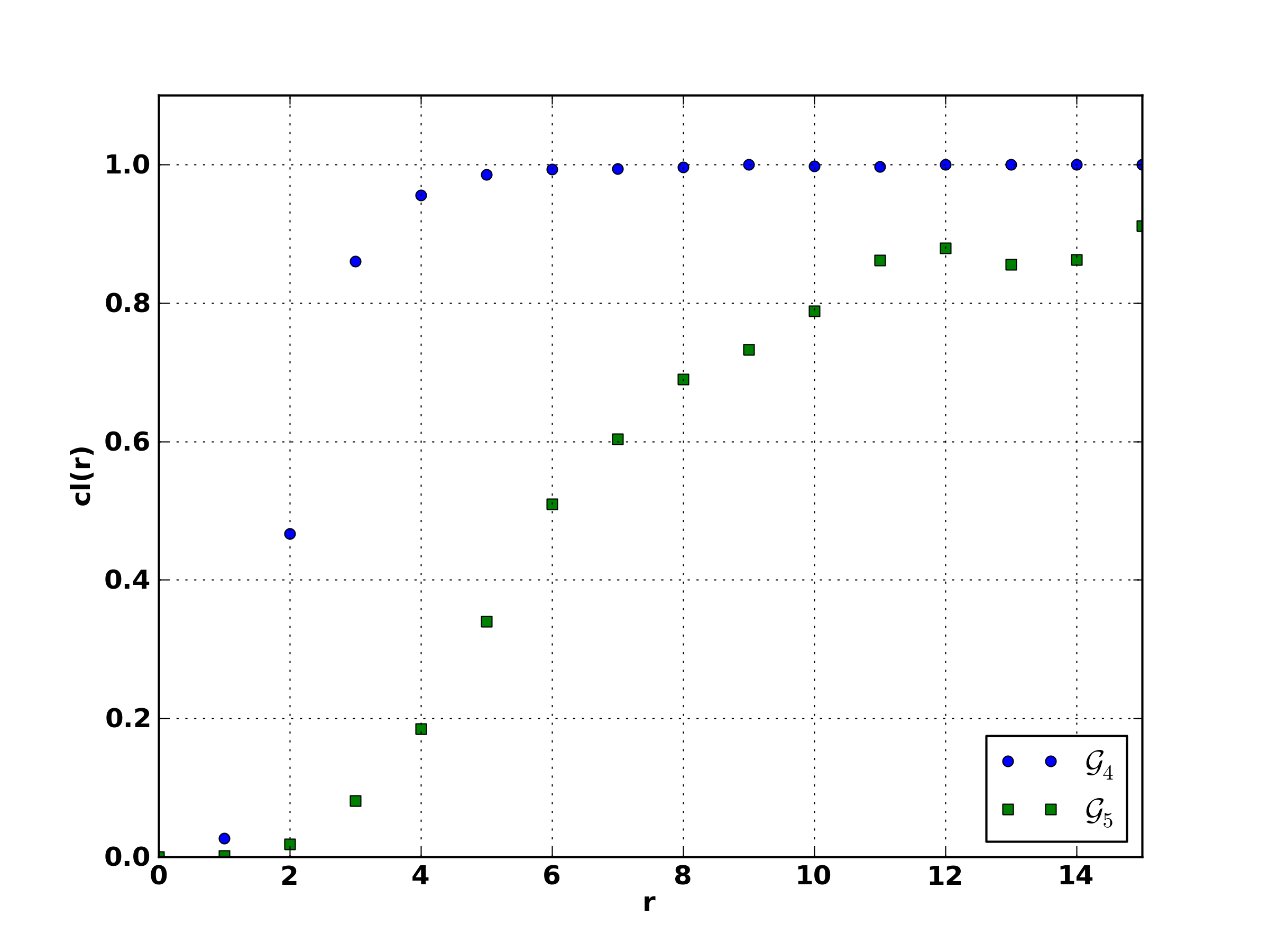
Figure 5 plots clustering function (1) of subgraphs of the first university network (see Sect 2.) sampled as follows. 𝒒1subscript𝒒1{\cal G}_{1} is the subgraph that includes all vertices of degree not larger than 505050. It has n0=7165subscript𝑛07165n_{0}=7165 vertices. 𝒒2subscript𝒒2{\cal G}_{2} is a subgraph induced by n0subscript𝑛0n_{0} vertices drawn uniformly at random (without replacement) from the vertices of degree not larger than 150150150. 𝒒3subscript𝒒3{\cal G}_{3} is a subgraph of induced by n0subscript𝑛0n_{0} vertices drawn uniformly at random (without replacement) from the set of all vertices. Now all three graphs have the same number of vertices.

Refer to caption
Figure 5: Sampling subgraphs with degree constraints.

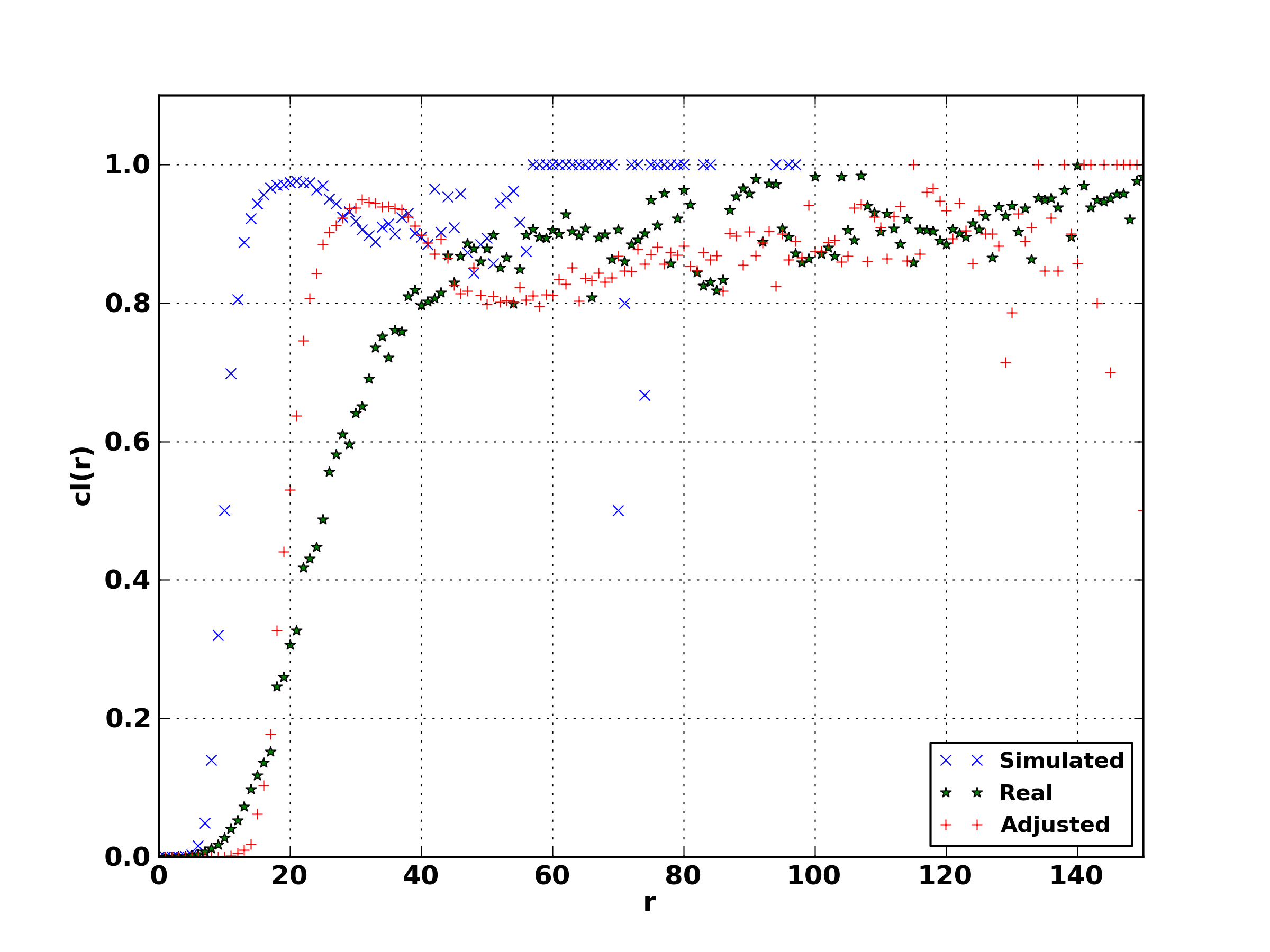
In Figure 6 we plot two subgraphs of the French actor network (data from [29]). The subgraph 𝒒4subscript𝒒4{\cal G}_{4} is induced by the set of marked vertices obtained as follows: we put a mark on each vertex v𝑣v with probability dβˆ’Ο„β€‹(v)superscriptπ‘‘πœπ‘£d^{-\tau}(v) and independently of the other vertices. Choosing Ο„=0.5𝜏0.5\tau=0.5 we obtain a random subgraph denoted 𝒒4subscript𝒒4{\cal G}_{4}. In our case the realized number of marked vertices n1=8871subscript𝑛18871n_{1}=8871. 𝒒5subscript𝒒5{\cal G}_{5} is the subgraph of the French actor network induced by n1subscript𝑛1n_{1} vertices drawn uniformly at random (without replacement) from the set of all vertices. Now both subgraphs have the same number of vertices, but the degree sequence of 𝒒4subscript𝒒4{\cal G}_{4} is much more regular than that of 𝒒5subscript𝒒5{\cal G}_{5}.

Refer to caption
Figure 6: Sampling a subgraph with a randomized degree constraint.

Finally, we examine how well a random intersection graph fits the real data. For this purpose we consider a memoryless actor network obtained as follows. Assume every actor of a given actor graph has forgotten about the titles of movies he or she acted in and only remembers the number of movies.

We first simulate an instance of the active memoryless graph where each actor chooses films independently and uniformly at random from a given set of m~~π‘š{\tilde{m}} films so that the number of films chosen by each actor is the same as in the true actor graph. In the active memoryless graph all films have equal chances to be selected by any of actors. We remark that in the case where m~=m~π‘šπ‘š{\tilde{m}}=m, i.e., the number of films in the active memoryless graph is the same as in the real underlying actor network, the expected degree of the memoryless graph does not match the average degree of the real network. We can easily adjust the number of films (of the memoryless graph) so that these degrees match. We denote this number mβ€²superscriptπ‘šβ€²m^{\prime} and call the active memoryless graph with m~=mβ€²~π‘šsuperscriptπ‘šβ€²{\tilde{m}}=m^{\prime} adjusted one. In Figure 7 we plot clustering function (1) of two instances of memoryless graphs for comparison with the underlying French actor network: one with the true number of films and another with the adjusted number of films.

We secondly simulate an instance of the inhomogeneous memoryless graph where an actor visubscript𝑣𝑖v_{i} chooses the film wjsubscript𝑀𝑗w_{j} with probability ai​bj​Mβˆ’1subscriptπ‘Žπ‘–subscript𝑏𝑗superscript𝑀1a_{i}b_{j}M^{-1} independently for each i𝑖i and j𝑗j. Here the numbers ai,bjsubscriptπ‘Žπ‘–subscript𝑏𝑗a_{i},b_{j} are observed characteristics of the underlying actor network: visubscript𝑣𝑖v_{i} acted in aisubscriptπ‘Žπ‘–a_{i} films; bjsubscript𝑏𝑗b_{j} actors acted in the film wjsubscript𝑀𝑗w_{j}. M=βˆ‘1≀i≀nai=βˆ‘1≀j≀mbj𝑀subscript1𝑖𝑛subscriptπ‘Žπ‘–subscript1π‘—π‘šsubscript𝑏𝑗M=\sum_{1\leq i\leq n}a_{i}=\sum_{1\leq j\leq m}b_{j} is the total number of links of the bipartite graph where actors are linked to films. In Figure 8 we plot clustering function (1) of an instance of the inhomogeneous memoryless graph of the French actor network. Here we observe a remarkable accuracy of the approximation of the real clustering function by that of the memoryless graph. We remark that in comparison with active memoryless graphs of Figure 7, that only use the data a1,…,ansubscriptπ‘Ž1…subscriptπ‘Žπ‘›a_{1},\dots,a_{n}, the inhomogeneous memoryless graph of Figure 8 uses, in addition, the numbers b1,…,bmsubscript𝑏1…subscriptπ‘π‘šb_{1},\dots,b_{m}.

We remark that Theorems 1, 2 and 3 establish a first order asymptotics to the clustering function c​l​(β‹…)𝑐𝑙⋅cl(\cdot) of random intersection graphs having a square integrable asymptotic degree distribution. An interesting question were about a power law random intersection graph whose asymptotic degree distribution has infinite second moment: Is there a limiting shape of the clustering function for nβ†’+βˆžβ†’π‘›n\to+\infty in this case? Is there a theoretically valid approximation to the clustering function that explains the gradual slope of c​l​(β‹…)𝑐𝑙⋅cl(\cdot) of observed empirical plots? It would also be interesting to learn about a higher order asymptotics of the clustering function c​l​(β‹…)𝑐𝑙⋅cl(\cdot) that refines results of Theorems 1, 3 and could perhaps better explain the empirical data.

Refer to caption
Figure 7: The French actor network and two simulated active memoryless networks.
Refer to caption
Figure 8: The French actor network and a simulated inhomogeneous memoryless network.

5 Proofs

The section is organized as follows: we first we formulate two auxiliary lemmas, then we prove Theorems 1, 2 and 3.

Lemma 1.

(See, e.g., [25]) Let S=𝕀1+𝕀2+β‹―+𝕀n𝑆subscript𝕀1subscript𝕀2β‹―subscript𝕀𝑛S={\mathbb{I}}_{1}+{\mathbb{I}}_{2}+\dots+{\mathbb{I}}_{n} be the sum of independent random indicators with probabilities 𝐏​(𝕀i=1)=pi𝐏subscript𝕀𝑖1subscript𝑝𝑖{\bf{P}}({\mathbb{I}}_{i}=1)=p_{i}. Let ΛΛ\Lambda be Poisson random variable with mean p1+β‹―+pnsubscript𝑝1β‹―subscript𝑝𝑛p_{1}+\dots+p_{n}. The total variation distance between the distributions PSsubscript𝑃𝑆P_{S} of PΞ›subscript𝑃ΛP_{\Lambda} of S𝑆S and ΛΛ\Lambda

supAβŠ‚{0,1,2​…}|𝐏​(S∈A)βˆ’πβ€‹(Ξ›βˆˆA)|β‰€βˆ‘ipi2.subscriptsupremum𝐴012…𝐏𝑆𝐴𝐏Λ𝐴subscript𝑖superscriptsubscript𝑝𝑖2\sup_{A\subset\{0,1,2\dots\}}|{\bf{P}}(S\in A)-{\bf{P}}(\Lambda\in A)|\leq\sum_{i}p_{i}^{2}. (14)
Lemma 2.

([7]) Given integers 1≀s≀d1≀d2≀m1𝑠subscript𝑑1subscript𝑑2π‘š1\leq s\leq d_{1}\leq d_{2}\leq m, let D1,D2subscript𝐷1subscript𝐷2D_{1},D_{2} be independent random subsets of the set W={1,…,m}π‘Š1β€¦π‘šW=\{1,\dots,m\} such that D1subscript𝐷1D_{1} (respectively D2subscript𝐷2D_{2}) is uniformly distributed in the class of subsets of Wπ‘ŠW of size d1subscript𝑑1d_{1} (respectively d2subscript𝑑2d_{2}). The probabilities pβ€²:=𝐏​(|D1∩D2|=s)assignsuperscript𝑝′𝐏subscript𝐷1subscript𝐷2𝑠p^{\prime}:={\bf{P}}(|D_{1}\cap D_{2}|=s) and pβ€²β€²:=𝐏​(|D1∩D2|β‰₯s)assignsuperscript𝑝′′𝐏subscript𝐷1subscript𝐷2𝑠p^{\prime\prime}:={\bf{P}}(|D_{1}\cap D_{2}|\geq s) satisfy

(1βˆ’(d1βˆ’s)​(d2βˆ’s)m+1βˆ’d1)​pd1,d2,sβˆ—β‰€p′≀p′′≀pd1,d2,sβˆ—,1subscript𝑑1𝑠subscript𝑑2π‘ π‘š1subscript𝑑1subscriptsuperscript𝑝subscript𝑑1subscript𝑑2𝑠superscript𝑝′superscript𝑝′′subscriptsuperscript𝑝subscript𝑑1subscript𝑑2𝑠\left(1-\frac{(d_{1}-s)(d_{2}-s)}{m+1-d_{1}}\right)p^{*}_{d_{1},d_{2},s}\ \leq\ p^{\prime}\ \leq\ p^{\prime\prime}\leq\ p^{*}_{d_{1},d_{2},s}, (15)

Here we denote pd1,d2,sβˆ—=(d1s)​(d2s)​(ms)βˆ’1subscriptsuperscript𝑝subscript𝑑1subscript𝑑2𝑠binomialsubscript𝑑1𝑠binomialsubscript𝑑2𝑠superscriptbinomialπ‘šπ‘ 1p^{*}_{d_{1},d_{2},s}={\tbinom{d_{1}}{s}}{\tbinom{d_{2}}{s}}{\tbinom{m}{s}}^{-1}.

5.1. Active graph. By Xi=Xn​isubscript𝑋𝑖subscript𝑋𝑛𝑖X_{i}=X_{ni} we denote the size of the set Disubscript𝐷𝑖D_{i} in G(n)subscript𝐺𝑛G_{(n)}. Furthermore, we write Zi=Zn​i=Ξ²nβˆ’1/2​Xn​isubscript𝑍𝑖subscript𝑍𝑛𝑖superscriptsubscript𝛽𝑛12subscript𝑋𝑛𝑖Z_{i}=Z_{ni}=\beta_{n}^{-1/2}X_{ni} and put Z01:=Zassignsubscript𝑍01𝑍Z_{01}:=Z. We denote zΒ―k=𝐄​Zn​1ksubscriptΒ―π‘§π‘˜π„superscriptsubscript𝑍𝑛1π‘˜{\bar{z}}_{k}={\bf{E}}Z_{n1}^{k} and introduce the function

t→φ​(t)=supnβ‰₯0𝐄​Zn​12​𝕀{Zn​1β‰₯t}.β†’π‘‘πœ‘π‘‘subscriptsupremum𝑛0𝐄superscriptsubscript𝑍𝑛12subscript𝕀subscript𝑍𝑛1𝑑t\to\varphi(t)=\sup_{n\geq 0}{\bf{E}}Z_{n1}^{2}{\mathbb{I}}_{\{Z_{n1}\geq t\}}. (16)

We remark that conditions (i), (ii-2) imply φ​(t)=o​(1)πœ‘π‘‘π‘œ1\varphi(t)=o(1) as tβ†’+βˆžβ†’π‘‘t\to+\infty (see, e.g., [7]) and zβˆ—2:=supnβ‰₯0𝐄​Zn​12<∞assignsubscript𝑧absent2subscriptsupremum𝑛0𝐄superscriptsubscript𝑍𝑛12z_{*2}:=\sup_{n\geq 0}{\bf{E}}Z_{n1}^{2}<\infty. By 𝐏~~𝐏{\tilde{\bf{P}}} and 𝐄~~𝐄{\tilde{\bf{E}}} we denote the conditional probability and expectation given X1subscript𝑋1X_{1}, X2subscript𝑋2X_{2}. By 𝐏~β€²superscript~𝐏′{\tilde{\bf{P}}}^{\prime} and 𝐄~β€²superscript~𝐄′{\tilde{\bf{E}}}^{\prime} we denote the conditional probability and expectation given D1subscript𝐷1D_{1}, D2subscript𝐷2D_{2}. We introduce events π’œ={v1∼v2}π’œsimilar-tosubscript𝑣1subscript𝑣2{\cal A}=\{v_{1}\sim v_{2}\}, π’œi={|D1∩D2|=i}subscriptπ’œπ‘–subscript𝐷1subscript𝐷2𝑖{\cal A}_{i}=\{|D_{1}\cap D_{2}|=i\} and probabilities

pi​(r)=𝐏​(π’œi∩{d12=r}),subscriptπ‘π‘–π‘Ÿπsubscriptπ’œπ‘–subscript𝑑12π‘Ÿp_{i}(r)={\bf{P}}({\cal A}_{i}\cap\{d_{12}=r\}),

By fr​(Ξ»)=eβˆ’Ξ»β€‹Ξ»r/r!subscriptπ‘“π‘Ÿπœ†superscriptπ‘’πœ†superscriptπœ†π‘Ÿπ‘Ÿf_{r}(\lambda)=e^{-\lambda}\lambda^{r}/r! we denote the Poisson probability.

Proof of Theorems 1 and 2.

We have

c​l​(r)=𝐏​(π’œ|d12=r)=𝐏​(π’œβˆ©{d12=r})𝐏​(d12=r).π‘π‘™π‘Ÿπconditionalπ’œsubscript𝑑12π‘Ÿππ’œsubscript𝑑12π‘Ÿπsubscript𝑑12π‘Ÿcl(r)={\bf{P}}({\cal A}|d_{12}=r)=\frac{{\bf{P}}({\cal A}\cap\{d_{12}=r\})}{{\bf{P}}(d_{12}=r)}. (17)

In order to evaluate the numerator we write π’œ=βˆͺiβ‰₯1π’œiπ’œsubscript𝑖1subscriptπ’œπ‘–{\cal A}=\cup_{i\geq 1}{\cal A}_{i} and apply the total probability formula

𝐏​(π’œβˆ©{d12=r})=βˆ‘iβ‰₯1pi​(r)=βˆ‘1≀i≀kpi​(r)+Rk​(r).ππ’œsubscript𝑑12π‘Ÿsubscript𝑖1subscriptπ‘π‘–π‘Ÿsubscript1π‘–π‘˜subscriptπ‘π‘–π‘Ÿsubscriptπ‘…π‘˜π‘Ÿ{\bf{P}}({\cal A}\cap\{d_{12}=r\})=\sum_{i\geq 1}p_{i}(r)=\sum_{1\leq i\leq k}p_{i}(r)+R_{k}(r). (18)

Here Rk​(r)=βˆ‘i>kpi​(r)≀𝐏​(|D1∩D2|β‰₯k+1)subscriptπ‘…π‘˜π‘Ÿsubscriptπ‘–π‘˜subscriptπ‘π‘–π‘Ÿπsubscript𝐷1subscript𝐷2π‘˜1R_{k}(r)=\sum_{i>k}p_{i}(r)\leq{\bf{P}}(|D_{1}\cap D_{2}|\geq k+1). Similarly we expand the denominator of (17)

𝐏​(d12=r)=βˆ‘iβ‰₯0pi​(r)=βˆ‘0≀i≀kpi​(r)+Rk​(r).𝐏subscript𝑑12π‘Ÿsubscript𝑖0subscriptπ‘π‘–π‘Ÿsubscript0π‘–π‘˜subscriptπ‘π‘–π‘Ÿsubscriptπ‘…π‘˜π‘Ÿ{\bf{P}}(d_{12}=r)=\sum_{i\geq 0}p_{i}(r)=\sum_{0\leq i\leq k}p_{i}(r)+R_{k}(r). (19)

In order to prove Theorem 1 we choose k=1π‘˜1k=1 in (18), (19) and invoke the asymptotic expressions of pi​(r)subscriptπ‘π‘–π‘Ÿp_{i}(r) and the upper bound for 𝐏​(|D1∩D2|β‰₯k+1)𝐏subscript𝐷1subscript𝐷2π‘˜1{\bf{P}}(|D_{1}\cap D_{2}|\geq k+1) shown in Lemma 3. Then, observing that as nβ†’+βˆžβ†’π‘›n\to+\infty we have zΒ―k=zk+o​(1)subscriptΒ―π‘§π‘˜subscriptπ‘§π‘˜π‘œ1{\bar{z}}_{k}=z_{k}+o(1), for k=1,2π‘˜12k=1,2, and Ξ±=Ξ²βˆ’1/2​z1/z2+o​(1)𝛼superscript𝛽12subscript𝑧1subscript𝑧2π‘œ1\alpha=\beta^{-1/2}z_{1}/z_{2}+o(1) (see (6)), we obtain (7).

Theorem 2 is obtained in the same way, but now we choose k=2π‘˜2k=2. ∎

Given a sequence of random variables {Yn}subscriptπ‘Œπ‘›\{Y_{n}\} and r=0,1,β€¦π‘Ÿ01…r=0,1,\dots we write Ynβ‰ΊOrprecedessubscriptπ‘Œπ‘›subscriptπ‘‚π‘ŸY_{n}\prec O_{r} to denote the fact that 𝐄​|Yn|=O​(nβˆ’2)𝐄subscriptπ‘Œπ‘›π‘‚superscript𝑛2{\bf{E}}|Y_{n}|=O(n^{-2}), for r=0,1π‘Ÿ01r=0,1, and 𝐄​|Yn|=O​(nβˆ’2​βnβˆ’1/2)+o​(nβˆ’2)𝐄subscriptπ‘Œπ‘›π‘‚superscript𝑛2superscriptsubscript𝛽𝑛12π‘œsuperscript𝑛2{\bf{E}}|Y_{n}|=O(n^{-2}\beta_{n}^{-1/2})+o(n^{-2}), for rβ‰₯2π‘Ÿ2r\geq 2.

Lemma 3.

Assume that Ξ²nβ†’Ξ²βˆˆ(0,+∞]β†’subscript𝛽𝑛𝛽0\beta_{n}\to\beta\in(0,+\infty]. Suppose that (i), (ii-2) hold. Denote Ξ›1=Ξ²nβˆ’1/2​zΒ―1subscriptΞ›1superscriptsubscript𝛽𝑛12subscript¯𝑧1\Lambda_{1}=\beta_{n}^{-1/2}{\bar{z}}_{1} and Ξ›2=zΒ―2βˆ’Ξ²nβˆ’1/2​zΒ―1subscriptΞ›2subscript¯𝑧2superscriptsubscript𝛽𝑛12subscript¯𝑧1\Lambda_{2}={\bar{z}}_{2}-\beta_{n}^{-1/2}{\bar{z}}_{1}. We have as nβ†’+βˆžβ†’π‘›n\to+\infty

p0​(0)=1βˆ’o​(1),p0​(r)=o​(nβˆ’2),rβ‰₯3,formulae-sequencesubscript𝑝001π‘œ1formulae-sequencesubscript𝑝0π‘Ÿπ‘œsuperscript𝑛2π‘Ÿ3\displaystyle p_{0}(0)=1-o(1),\qquad p_{0}(r)=o(n^{-2}),\qquad\ r\geq 3, (20)
p0​(r)=nβˆ’r​(r!)βˆ’1​Λ2r​zΒ―r2+o​(nβˆ’r),r=1,2,formulae-sequencesubscript𝑝0π‘Ÿsuperscriptπ‘›π‘Ÿsuperscriptπ‘Ÿ1superscriptsubscriptΞ›2π‘ŸsuperscriptsubscriptΒ―π‘§π‘Ÿ2π‘œsuperscriptπ‘›π‘Ÿπ‘Ÿ12\displaystyle p_{0}(r)=n^{-r}(r!)^{-1}\Lambda_{2}^{r}{\bar{z}}_{r}^{2}+o(n^{-r}),\qquad\quad\ \quad r=1,2, (21)
p1​(r)=nβˆ’1​zΒ―12​fr​(Ξ›1)+Or,rβ‰₯0,formulae-sequencesubscript𝑝1π‘Ÿsuperscript𝑛1superscriptsubscript¯𝑧12subscriptπ‘“π‘ŸsubscriptΞ›1subscriptπ‘‚π‘Ÿπ‘Ÿ0\displaystyle p_{1}(r)=n^{-1}{\bar{z}}_{1}^{2}f_{r}(\Lambda_{1})+O_{r},\qquad\qquad\qquad\quad r\geq 0, (22)
p2​(r)=2βˆ’1​nβˆ’2​fr​(2​Λ1)​Λ22+O2,rβ‰₯0.formulae-sequencesubscript𝑝2π‘Ÿsuperscript21superscript𝑛2subscriptπ‘“π‘Ÿ2subscriptΞ›1superscriptsubscriptΞ›22subscript𝑂2π‘Ÿ0\displaystyle p_{2}(r)=2^{-1}n^{-2}f_{r}(2\Lambda_{1})\Lambda_{2}^{2}+O_{2},\qquad\qquad\quad r\geq 0. (23)

Furthermore, we have

𝐏​(|D1∩D2|β‰₯3)=o​(nβˆ’2)and𝐏​(|D1∩D2|β‰₯k)=O​(nβˆ’k),k=1,2.formulae-sequence𝐏subscript𝐷1subscript𝐷23π‘œsuperscript𝑛2andformulae-sequence𝐏subscript𝐷1subscript𝐷2π‘˜π‘‚superscriptπ‘›π‘˜π‘˜12{\bf{P}}(|D_{1}\cap D_{2}|\geq 3)=o(n^{-2})\qquad{\text{and}}\qquad{\bf{P}}(|D_{1}\cap D_{2}|\geq k)=O(n^{-k}),\quad k=1,2. (24)
Proof of Lemma 3.

Before the proof we introduce some notation and collect auxiliary inequalities. Then we give an outline of the proof. Afterwards we prove (20), (21) and (22), (23).

By cβˆ—subscript𝑐c_{*} we denote a generic positive constant. By 𝕀ℬsubscript𝕀ℬ{\mathbb{I}}_{\cal B} we denote the indicator of an event ℬℬ{\cal B} and write 𝕀¯ℬ=1βˆ’π•€β„¬subscript¯𝕀ℬ1subscript𝕀ℬ{\overline{\mathbb{I}}}_{\cal B}=1-{\mathbb{I}}_{\cal B}. In the proof we use several indicators

𝕀=𝕀{X1+X2<Ξ΅2​n​βn1/2},𝕀j=𝕀{Xj<0.5​Ρ2​n​βn1/2},π•€βˆ—j=𝕀{Xj≀βn1/2β€‹Ξ΅βˆ’1},\displaystyle{\mathbb{I}}\ \ ={\mathbb{I}}_{\{X_{1}+X_{2}<\varepsilon^{2}n\beta_{n}^{1/2}\}},\quad{\mathbb{I}}_{j}={\mathbb{I}}_{\{X_{j}<0.5\varepsilon^{2}n\beta_{n}^{1/2}\}},\quad{\mathbb{I}}_{*j}={\mathbb{I}}_{\{X_{j}\leq\beta_{n}^{1/2}\varepsilon^{-1}\}},
𝕀⋆j=𝕀{Xj≀Ρ​m},𝐈j=𝕀{Xj<m1/2​nβˆ’1/4},πˆβˆ—j=𝕀{Xj≀0.5​m}.formulae-sequencesubscript𝕀⋆absent𝑗subscript𝕀subscriptπ‘‹π‘—πœ€π‘šformulae-sequencesubscriptπˆπ‘—subscript𝕀subscript𝑋𝑗superscriptπ‘š12superscript𝑛14subscript𝐈absent𝑗subscript𝕀subscript𝑋𝑗0.5π‘š\displaystyle{\mathbb{I}}_{\star j}={\mathbb{I}}_{\{X_{j}\leq\varepsilon m\}},\qquad\qquad\ {\bf I}_{j}={\mathbb{I}}_{\{X_{j}<m^{1/2}n^{-1/4}\}},\quad{\bf I}_{*j}={\mathbb{I}}_{\{X_{j}\leq 0.5m\}}.

Some of them depend on Ξ΅>0πœ€0\varepsilon>0, value of which will be clear from the context. We denote

q~0=nβˆ’2​Λ2​Z1​Z2,q~1=nβˆ’1​Λ1,q~2=2​nβˆ’1​Λ1,formulae-sequencesubscript~π‘ž0superscript𝑛2subscriptΞ›2subscript𝑍1subscript𝑍2formulae-sequencesubscript~π‘ž1superscript𝑛1subscriptΞ›1subscript~π‘ž22superscript𝑛1subscriptΞ›1{\tilde{q}}_{0}=n^{-2}\Lambda_{2}Z_{1}Z_{2},\qquad{\tilde{q}}_{1}=n^{-1}\Lambda_{1},\qquad{\tilde{q}}_{2}=2n^{-1}\Lambda_{1}, (25)

and, for i=1,2𝑖12i=1,2 we write

Ξ»~i=n​q~i,Ξ»i=(nβˆ’2)​qi,qi=𝐏~′​(v1∼v3,v2∼v3)β€‹π•€π’œi,Ο°i=(X1)i​(X2)i/(i!​(m)i).formulae-sequencesubscript~πœ†π‘–π‘›subscript~π‘žπ‘–formulae-sequencesubscriptπœ†π‘–π‘›2subscriptπ‘žπ‘–formulae-sequencesubscriptπ‘žπ‘–superscript~𝐏′formulae-sequencesimilar-tosubscript𝑣1subscript𝑣3similar-tosubscript𝑣2subscript𝑣3subscript𝕀subscriptπ’œπ‘–subscriptitalic-ϰ𝑖subscriptsubscript𝑋1𝑖subscriptsubscript𝑋2𝑖𝑖subscriptπ‘šπ‘–{\tilde{\lambda}}_{i}=n{\tilde{q}}_{i},\qquad\lambda_{i}=(n-2)q_{i},\qquad q_{i}={\tilde{\bf{P}}}^{\prime}(v_{1}\sim v_{3},v_{2}\sim v_{3}){\mathbb{I}}_{{\cal A}_{i}},\qquad\varkappa_{i}=(X_{1})_{i}(X_{2})_{i}/(i!(m)_{i}).

We note that (15) implies

Ο°i​(1βˆ’X1​X2/(mβˆ’X1))≀𝐏~​(π’œi)≀ϰi.subscriptitalic-ϰ𝑖1subscript𝑋1subscript𝑋2π‘šsubscript𝑋1~𝐏subscriptπ’œπ‘–subscriptitalic-ϰ𝑖\varkappa_{i}(1-X_{1}X_{2}/(m-X_{1}))\leq{\tilde{\bf{P}}}({\cal A}_{i})\leq\varkappa_{i}. (26)

In particular, we have

𝐏~​(π’œi)≀𝐏~​(π’œi)​(𝐈1β€‹πˆ2+𝐈¯1+𝐈¯2)≀ϰiβ€‹πˆ1β€‹πˆ2+𝐈¯1+𝐈¯2≀nβˆ’i/2+𝐈¯1+𝐈¯2.~𝐏subscriptπ’œπ‘–~𝐏subscriptπ’œπ‘–subscript𝐈1subscript𝐈2subscript¯𝐈1subscript¯𝐈2subscriptitalic-ϰ𝑖subscript𝐈1subscript𝐈2subscript¯𝐈1subscript¯𝐈2superscript𝑛𝑖2subscript¯𝐈1subscript¯𝐈2{\tilde{\bf{P}}}({\cal A}_{i})\leq{\tilde{\bf{P}}}({\cal A}_{i})({\bf I}_{1}{\bf I}_{2}+{\overline{\bf I}}_{1}+{\overline{\bf I}}_{2})\leq\varkappa_{i}{\bf I}_{1}{\bf I}_{2}+{\overline{\bf I}}_{1}+{\overline{\bf I}}_{2}\leq n^{-i/2}+{\overline{\bf I}}_{1}+{\overline{\bf I}}_{2}. (27)

We will use the following properties of the function Ξ»β†’fr​(Ξ»)β†’πœ†subscriptπ‘“π‘Ÿπœ†\lambda\to f_{r}(\lambda). For r=0,1,β€¦π‘Ÿ01…r=0,1,\dots, it follows from the mean value theorem fr​(t)βˆ’fr​(s)=fr′​(ΞΎ)​(tβˆ’s)subscriptπ‘“π‘Ÿπ‘‘subscriptπ‘“π‘Ÿπ‘ superscriptsubscriptπ‘“π‘Ÿβ€²πœ‰π‘‘π‘ f_{r}(t)-f_{r}(s)=f_{r}^{\prime}(\xi)(t-s), where 0<s≀ξ≀t0π‘ πœ‰π‘‘0<s\leq\xi\leq t, combined with inequalities |fr′​(ΞΎ)|≀1superscriptsubscriptπ‘“π‘Ÿβ€²πœ‰1|f_{r}^{\prime}(\xi)|\leq 1 and |f2+r′​(ΞΎ)|≀ξsuperscriptsubscript𝑓2π‘Ÿβ€²πœ‰πœ‰|f_{2+r}^{\prime}(\xi)|\leq\xi that

|fr​(s)βˆ’fr​(t)|≀|sβˆ’t|and|f2+r​(s)βˆ’f2+r​(t)|≀(s+t)​|sβˆ’t|.formulae-sequencesubscriptπ‘“π‘Ÿπ‘ subscriptπ‘“π‘Ÿπ‘‘π‘ π‘‘andsubscript𝑓2π‘Ÿπ‘ subscript𝑓2π‘Ÿπ‘‘π‘ π‘‘π‘ π‘‘|f_{r}(s)-f_{r}(t)|\leq|s-t|\qquad{\text{and}}\qquad|f_{2+r}(s)-f_{2+r}(t)|\leq(s+t)|s-t|. (28)

Now we outline the proof. In order to evaluate pi​(r)subscriptπ‘π‘–π‘Ÿp_{i}(r) we write

pi​(r)=𝐄​(𝐄~′​(π•€π’œi​𝕀{d12=r}))=𝐄​(π•€π’œi​𝐄~′​𝕀{d12=r})=𝐄​(π•€π’œi​𝐏~′​(d12=r))subscriptπ‘π‘–π‘Ÿπ„superscript~𝐄′subscript𝕀subscriptπ’œπ‘–subscript𝕀subscript𝑑12π‘Ÿπ„subscript𝕀subscriptπ’œπ‘–superscript~𝐄′subscript𝕀subscript𝑑12π‘Ÿπ„subscript𝕀subscriptπ’œπ‘–superscript~𝐏′subscript𝑑12π‘Ÿp_{i}(r)={\bf{E}}({\tilde{\bf{E}}}^{\prime}({\mathbb{I}}_{{\cal A}_{i}}{\mathbb{I}}_{\{d_{12}=r\}}))={\bf{E}}({\mathbb{I}}_{{\cal A}_{i}}{\tilde{\bf{E}}}^{\prime}{\mathbb{I}}_{\{d_{12}=r\}})={\bf{E}}({\mathbb{I}}_{{\cal A}_{i}}{\tilde{\bf{P}}}^{\prime}(d_{12}=r)) (29)

and observe that, given D1,D2subscript𝐷1subscript𝐷2D_{1},D_{2} satisfying |D1∩D2|=isubscript𝐷1subscript𝐷2𝑖|D_{1}\cap D_{2}|=i, the random variable

d12=βˆ‘3≀j≀n𝕀{v1∼vj}​𝕀{v2∼vj}subscript𝑑12subscript3𝑗𝑛subscript𝕀similar-tosubscript𝑣1subscript𝑣𝑗subscript𝕀similar-tosubscript𝑣2subscript𝑣𝑗d_{12}=\sum_{3\leq j\leq n}{\mathbb{I}}_{\{v_{1}\sim v_{j}\}}{\mathbb{I}}_{\{v_{2}\sim v_{j}\}}

has binomial distribution 𝐁𝐒𝐧​(nβˆ’2,qi)𝐁𝐒𝐧𝑛2subscriptπ‘žπ‘–{\bf{Bin}}(n-2,q_{i}). We first approximate 𝐏~′​(d12=r)superscript~𝐏′subscript𝑑12π‘Ÿ{\tilde{\bf{P}}}^{\prime}(d_{12}=r) in (29) by the Poisson probability fr​(Ξ»i)subscriptπ‘“π‘Ÿsubscriptπœ†π‘–f_{r}(\lambda_{i}). Then, we approximate Ξ»isubscriptπœ†π‘–\lambda_{i} by Ξ»~isubscript~πœ†π‘–{\tilde{\lambda}}_{i}, and fr​(Ξ»i)subscriptπ‘“π‘Ÿsubscriptπœ†π‘–f_{r}(\lambda_{i}) by fr​(Ξ»~i)subscriptπ‘“π‘Ÿsubscript~πœ†π‘–f_{r}({\tilde{\lambda}}_{i}). We obtain

pi​(r)=𝐄​(π•€π’œi​fr​(Ξ»~i))+𝐄​(π•€π’œi​Δr,i)=𝐄​(𝐏~​(π’œi)​fr​(Ξ»~i))+𝐄​(π•€π’œi​Δr,i),subscriptπ‘π‘–π‘Ÿπ„subscript𝕀subscriptπ’œπ‘–subscriptπ‘“π‘Ÿsubscript~πœ†π‘–π„subscript𝕀subscriptπ’œπ‘–subscriptΞ”π‘Ÿπ‘–π„~𝐏subscriptπ’œπ‘–subscriptπ‘“π‘Ÿsubscript~πœ†π‘–π„subscript𝕀subscriptπ’œπ‘–subscriptΞ”π‘Ÿπ‘–p_{i}(r)={\bf{E}}({\mathbb{I}}_{{\cal A}_{i}}f_{r}({\tilde{\lambda}}_{i}))+{\bf{E}}({\mathbb{I}}_{{\cal A}_{i}}\Delta_{r,i})={\bf{E}}({\tilde{\bf{P}}}({\cal A}_{i})f_{r}({\tilde{\lambda}}_{i}))+{\bf{E}}({\mathbb{I}}_{{\cal A}_{i}}\Delta_{r,i}), (30)

where, for |D1∩D2|=isubscript𝐷1subscript𝐷2𝑖|D_{1}\cap D_{2}|=i, we denote

Ξ”r,i:=𝐏~′​(d12=r)βˆ’fr​(Ξ»~i)=Ξ”r,iβ€²+Ξ”r,iβ€²β€²,assignsubscriptΞ”π‘Ÿπ‘–superscript~𝐏′subscript𝑑12π‘Ÿsubscriptπ‘“π‘Ÿsubscript~πœ†π‘–superscriptsubscriptΞ”π‘Ÿπ‘–β€²superscriptsubscriptΞ”π‘Ÿπ‘–β€²β€²\displaystyle\Delta_{r,i}:={\tilde{\bf{P}}}^{\prime}(d_{12}=r)-f_{r}({\tilde{\lambda}}_{i})=\Delta_{r,i}^{\prime}+\Delta_{r,i}^{\prime\prime}, (31)
Ξ”r,iβ€²=𝐏~′​(d12=r)βˆ’fr​(Ξ»i),Ξ”r,iβ€²β€²=fr​(Ξ»i)βˆ’fr​(Ξ»~i).formulae-sequencesuperscriptsubscriptΞ”π‘Ÿπ‘–β€²superscript~𝐏′subscript𝑑12π‘Ÿsubscriptπ‘“π‘Ÿsubscriptπœ†π‘–superscriptsubscriptΞ”π‘Ÿπ‘–β€²β€²subscriptπ‘“π‘Ÿsubscriptπœ†π‘–subscriptπ‘“π‘Ÿsubscript~πœ†π‘–\displaystyle\Delta_{r,i}^{\prime}={\tilde{\bf{P}}}^{\prime}(d_{12}=r)-f_{r}(\lambda_{i}),\qquad\Delta_{r,i}^{\prime\prime}=f_{r}(\lambda_{i})-f_{r}({\tilde{\lambda}}_{i}).

Next we show that the remainder term 𝐄​(π•€π’œi​Δr,i)𝐄subscript𝕀subscriptπ’œπ‘–subscriptΞ”π‘Ÿπ‘–{\bf{E}}({\mathbb{I}}_{{\cal A}_{i}}\Delta_{r,i}) of (30) is negligible. For this purpose we estimate using LeCam’s lemma (see Lemma 1)

|Ξ”r,iβ€²|≀n​qi2,subscriptsuperscriptΞ”β€²π‘Ÿπ‘–π‘›subscriptsuperscriptπ‘ž2𝑖|\Delta^{\prime}_{r,i}|\leq nq^{2}_{i}, (32)

and estimate Ξ”r,iβ€²β€²superscriptsubscriptΞ”π‘Ÿπ‘–β€²β€²\Delta_{r,i}^{\prime\prime} combining (28) with the approximations qiβ‰ˆq~isubscriptπ‘žπ‘–subscript~π‘žπ‘–q_{i}\approx{\tilde{q}}_{i}. We briefly explain these approximations. Let {w1βˆ—,…,wiβˆ—}superscriptsubscript𝑀1…superscriptsubscript𝑀𝑖\{w_{1}^{*},\dots,w_{i}^{*}\} denote the intersection D1∩D2subscript𝐷1subscript𝐷2D_{1}\cap D_{2} provided it is non empty. Denote nj=|D3∩Dj|subscript𝑛𝑗subscript𝐷3subscript𝐷𝑗n_{j}=|D_{3}\cap D_{j}|, j=1,2𝑗12j=1,2. We split

q0=q01+q02,q1=q11+q12,q2=q21+q22+q23+q24,formulae-sequencesubscriptπ‘ž0subscriptπ‘ž01subscriptπ‘ž02formulae-sequencesubscriptπ‘ž1subscriptπ‘ž11subscriptπ‘ž12subscriptπ‘ž2subscriptπ‘ž21subscriptπ‘ž22subscriptπ‘ž23subscriptπ‘ž24q_{0}=q_{01}+q_{02},\qquad q_{1}=q_{11}+q_{12},\qquad q_{2}=q_{21}+q_{22}+q_{23}+q_{24},

where

q01=𝐏~′​(n1=1,n2=1)β€‹π•€π’œ0,q02=𝐏~′​(n1+n2β‰₯3,n1β‰₯1,n2β‰₯1)β€‹π•€π’œ0,formulae-sequencesubscriptπ‘ž01superscript~𝐏′formulae-sequencesubscript𝑛11subscript𝑛21subscript𝕀subscriptπ’œ0subscriptπ‘ž02superscript~𝐏′formulae-sequencesubscript𝑛1subscript𝑛23formulae-sequencesubscript𝑛11subscript𝑛21subscript𝕀subscriptπ’œ0\displaystyle q_{01}={\tilde{\bf{P}}}^{\prime}(n_{1}=1,n_{2}=1){\mathbb{I}}_{{\cal A}_{0}},\qquad\ q_{02}={\tilde{\bf{P}}}^{\prime}(n_{1}+n_{2}\geq 3,n_{1}\geq 1,n_{2}\geq 1){\mathbb{I}}_{{\cal A}_{0}},
q11=𝐏~′​(w1βˆ—βˆˆD3)β€‹π•€π’œ1,q12=𝐏~′​(w1βˆ—βˆ‰D3,n1β‰₯1,n2β‰₯1)β€‹π•€π’œ1,formulae-sequencesubscriptπ‘ž11superscript~𝐏′superscriptsubscript𝑀1subscript𝐷3subscript𝕀subscriptπ’œ1subscriptπ‘ž12superscript~𝐏′formulae-sequencesuperscriptsubscript𝑀1subscript𝐷3formulae-sequencesubscript𝑛11subscript𝑛21subscript𝕀subscriptπ’œ1\displaystyle q_{11}={\tilde{\bf{P}}}^{\prime}(w_{1}^{*}\in D_{3}){\mathbb{I}}_{{\cal A}_{1}},\qquad\quad\ \ \ \quad q_{12}={\tilde{\bf{P}}}^{\prime}(w_{1}^{*}\notin D_{3},n_{1}\geq 1,n_{2}\geq 1){\mathbb{I}}_{{\cal A}_{1}}, (33)
q21=𝐏~′​(w1βˆ—βˆˆD3,w2βˆ—βˆ‰D3)β€‹π•€π’œ2,q22=𝐏~′​(w1βˆ—βˆ‰D3,w2βˆ—βˆˆD3)β€‹π•€π’œ2,formulae-sequencesubscriptπ‘ž21superscript~𝐏′formulae-sequencesuperscriptsubscript𝑀1subscript𝐷3superscriptsubscript𝑀2subscript𝐷3subscript𝕀subscriptπ’œ2subscriptπ‘ž22superscript~𝐏′formulae-sequencesuperscriptsubscript𝑀1subscript𝐷3superscriptsubscript𝑀2subscript𝐷3subscript𝕀subscriptπ’œ2\displaystyle q_{21}={\tilde{\bf{P}}}^{\prime}(w_{1}^{*}\in D_{3},w_{2}^{*}\notin D_{3}){\mathbb{I}}_{{\cal A}_{2}},\quad q_{22}={\tilde{\bf{P}}}^{\prime}(w_{1}^{*}\notin D_{3},w_{2}^{*}\in D_{3}){\mathbb{I}}_{{\cal A}_{2}},
q23=𝐏~β€²(w1βˆ—,w2βˆ—βˆˆD3)π•€π’œ2,q24=𝐏~β€²(w1βˆ—,w2βˆ—βˆ‰D3,n1β‰₯1,n2β‰₯1)π•€π’œ2,\displaystyle q_{23}={\tilde{\bf{P}}}^{\prime}(w_{1}^{*},w_{2}^{*}\in D_{3}){\mathbb{I}}_{{\cal A}_{2}},\qquad\quad\ \ q_{24}={\tilde{\bf{P}}}^{\prime}(w_{1}^{*},w_{2}^{*}\notin D_{3},n_{1}\geq 1,n_{2}\geq 1){\mathbb{I}}_{{\cal A}_{2}},

and approximate q0β‰ˆq01β‰ˆq~0β€‹π•€π’œ0subscriptπ‘ž0subscriptπ‘ž01subscript~π‘ž0subscript𝕀subscriptπ’œ0q_{0}\approx q_{01}\approx{\tilde{q}}_{0}{\mathbb{I}}_{{\cal A}_{0}}, q1β‰ˆq11=q~1β€‹π•€π’œ1subscriptπ‘ž1subscriptπ‘ž11subscript~π‘ž1subscript𝕀subscriptπ’œ1q_{1}\approx q_{11}={\tilde{q}}_{1}{\mathbb{I}}_{{\cal A}_{1}} and q2β‰ˆq21+q22β‰ˆq~2β€‹π•€π’œ2subscriptπ‘ž2subscriptπ‘ž21subscriptπ‘ž22subscript~π‘ž2subscript𝕀subscriptπ’œ2q_{2}\approx q_{21}+q_{22}\approx{\tilde{q}}_{2}{\mathbb{I}}_{{\cal A}_{2}}.

Proof of (20), (21). In order to prove (20), (21) we show that

𝐄​(π•€π’œ0​Δr,0)=o​(nβˆ’r∧2),rβ‰₯0formulae-sequence𝐄subscript𝕀subscriptπ’œ0subscriptΞ”π‘Ÿ0π‘œsuperscriptπ‘›π‘Ÿ2π‘Ÿ0\displaystyle{\bf{E}}({\mathbb{I}}_{{\cal A}_{0}}\Delta_{r,0})=o(n^{-r\wedge 2}),\qquad r\geq 0 (34)
𝐄​(π•€π’œ0​fr​(Ξ»~0))=(r!)βˆ’1​𝐄​λ~0r+o​(nβˆ’r),r=0,1,2,formulae-sequence𝐄subscript𝕀subscriptπ’œ0subscriptπ‘“π‘Ÿsubscript~πœ†0superscriptπ‘Ÿ1𝐄superscriptsubscript~πœ†0π‘Ÿπ‘œsuperscriptπ‘›π‘Ÿπ‘Ÿ012\displaystyle{\bf{E}}({\mathbb{I}}_{{\cal A}_{0}}f_{r}({\tilde{\lambda}}_{0}))=(r!)^{-1}{\bf{E}}{\tilde{\lambda}}_{0}^{r}+o(n^{-r}),\qquad r=0,1,2, (35)
𝐄​(π•€π’œ0​fr​(Ξ»~0))=o​(nβˆ’2),rβ‰₯3.formulae-sequence𝐄subscript𝕀subscriptπ’œ0subscriptπ‘“π‘Ÿsubscript~πœ†0π‘œsuperscript𝑛2π‘Ÿ3\displaystyle{\bf{E}}({\mathbb{I}}_{{\cal A}_{0}}f_{r}({\tilde{\lambda}}_{0}))=o(n^{-2}),\qquad r\geq 3. (36)

We firstly prove (34). In the case where Ξ²<βˆžπ›½\beta<\infty we find n0>0subscript𝑛00n_{0}>0 such that Ξ²<2​βn𝛽2subscript𝛽𝑛\beta<2\beta_{n} for nβ‰₯n0𝑛subscript𝑛0n\geq n_{0}. In the case where Ξ²=+βˆžπ›½\beta=+\infty we find n0subscript𝑛0n_{0} such that Ξ²n>1subscript𝛽𝑛1\beta_{n}>1 for nβ‰₯n0𝑛subscript𝑛0n\geq n_{0}. In order to prove (34) we show that for any 0<Ξ΅<min⁑{0.5​β1/2,0.1}0πœ€0.5superscript𝛽120.10<\varepsilon<\min\{0.5\beta^{1/2},0.1\} and nβ‰₯n0𝑛subscript𝑛0n\geq n_{0} we have

𝐄​(π•€π’œ0​|Ξ”r,0|)≀cβˆ—β€‹nβˆ’3+cβˆ—β€‹nβˆ’r∧2​R1​(Ξ΅)+cβˆ—β€‹nβˆ’2β€‹Ξ΅βˆ’4​R2​(Ξ΅),𝐄subscript𝕀subscriptπ’œ0subscriptΞ”π‘Ÿ0subscript𝑐superscript𝑛3subscript𝑐superscriptπ‘›π‘Ÿ2subscript𝑅1πœ€subscript𝑐superscript𝑛2superscriptπœ€4subscript𝑅2πœ€\displaystyle{\bf{E}}({\mathbb{I}}_{{\cal A}_{0}}|\Delta_{r,0}|)\leq c_{*}n^{-3}+c_{*}n^{-r\wedge 2}R_{1}(\varepsilon)+c_{*}n^{-2}\varepsilon^{-4}R_{2}(\varepsilon), (37)
R1​(Ξ΅):=φ​(Ξ΅βˆ’1)+Ξ΅+mβˆ’1+nβˆ’1,R2​(Ξ΅):=φ​(0.5​Ρ2​n)​(1+Ξ΅βˆ’4​nβˆ’2).formulae-sequenceassignsubscript𝑅1πœ€πœ‘superscriptπœ€1πœ€superscriptπ‘š1superscript𝑛1assignsubscript𝑅2πœ€πœ‘0.5superscriptπœ€2𝑛1superscriptπœ€4superscript𝑛2\displaystyle R_{1}(\varepsilon):=\varphi(\varepsilon^{-1})+\varepsilon+m^{-1}+n^{-1},\qquad R_{2}(\varepsilon):=\varphi(0.5\varepsilon^{2}n)(1+\varepsilon^{-4}n^{-2}).

We remark that (37) combined with the relation limtβ†’+βˆžΟ†β€‹(t)=0subscriptβ†’π‘‘πœ‘π‘‘0\lim_{t\to+\infty}\varphi(t)=0 implies (34).

Let us prove (37). Given Ξ΅πœ€\varepsilon, we write Ξ”r,0=Ξ”r,0​𝕀+Ξ”r,0​𝕀¯subscriptΞ”π‘Ÿ0subscriptΞ”π‘Ÿ0𝕀subscriptΞ”π‘Ÿ0¯𝕀\Delta_{r,0}=\Delta_{r,0}{\mathbb{I}}+\Delta_{r,0}{\overline{\mathbb{I}}} and show that

𝐄​|Ξ”r,0|​𝕀¯≀𝐄​𝕀¯≀cβˆ—β€‹nβˆ’2β€‹Ξ΅βˆ’4​R2​(Ξ΅),𝐄subscriptΞ”π‘Ÿ0¯𝕀𝐄¯𝕀subscript𝑐superscript𝑛2superscriptπœ€4subscript𝑅2πœ€\displaystyle{\bf{E}}|\Delta_{r,0}|{\overline{\mathbb{I}}}\leq{\bf{E}}{\overline{\mathbb{I}}}\leq c_{*}n^{-2}\varepsilon^{-4}R_{2}(\varepsilon), (38)
π„β€‹π•€π’œ0​|Ξ”r,0|​𝕀≀cβˆ—β€‹nβˆ’3+cβˆ—β€‹nβˆ’r∧2​R1​(Ξ΅).𝐄subscript𝕀subscriptπ’œ0subscriptΞ”π‘Ÿ0𝕀subscript𝑐superscript𝑛3subscript𝑐superscriptπ‘›π‘Ÿ2subscript𝑅1πœ€\displaystyle{\bf{E}}{\mathbb{I}}_{{\cal A}_{0}}|\Delta_{r,0}|{\mathbb{I}}\leq c_{*}n^{-3}+c_{*}n^{-r\wedge 2}R_{1}(\varepsilon). (39)

The first inequality of (38) is obvious. In order to prove the second one we combine the inequalities

Ξ΅4​n2​𝐄​𝕀¯≀βnβˆ’1​𝐄​(X1+X2)2​𝕀¯≀2​βnβˆ’1​𝐄​(X12+X22)​𝕀¯=4​βnβˆ’1​𝐄​X12​𝕀¯,superscriptπœ€4superscript𝑛2𝐄¯𝕀superscriptsubscript𝛽𝑛1𝐄superscriptsubscript𝑋1subscript𝑋22¯𝕀2superscriptsubscript𝛽𝑛1𝐄superscriptsubscript𝑋12superscriptsubscript𝑋22¯𝕀4superscriptsubscript𝛽𝑛1𝐄superscriptsubscript𝑋12¯𝕀\varepsilon^{4}n^{2}{\bf{E}}{\overline{\mathbb{I}}}\leq\beta_{n}^{-1}{\bf{E}}(X_{1}+X_{2})^{2}{\overline{\mathbb{I}}}\leq 2\beta_{n}^{-1}{\bf{E}}(X_{1}^{2}+X_{2}^{2}){\overline{\mathbb{I}}}=4\beta_{n}^{-1}{\bf{E}}X_{1}^{2}{\overline{\mathbb{I}}},

which follow from Markov’s inequality, with the inequalities

Ξ²nβˆ’1​𝐄​X12​𝕀¯≀βnβˆ’1​𝐄​X12​(𝕀¯1+𝕀¯2)≀βnβˆ’1​𝐄​X12​(𝕀¯1+4β€‹Ξ΅βˆ’4​nβˆ’2​βnβˆ’1​X22​𝕀¯2)≀cβˆ—β€‹R2​(Ξ΅).superscriptsubscript𝛽𝑛1𝐄superscriptsubscript𝑋12¯𝕀superscriptsubscript𝛽𝑛1𝐄superscriptsubscript𝑋12subscript¯𝕀1subscript¯𝕀2superscriptsubscript𝛽𝑛1𝐄superscriptsubscript𝑋12subscript¯𝕀14superscriptπœ€4superscript𝑛2superscriptsubscript𝛽𝑛1superscriptsubscript𝑋22subscript¯𝕀2subscript𝑐subscript𝑅2πœ€\beta_{n}^{-1}{\bf{E}}X_{1}^{2}{\overline{\mathbb{I}}}\leq\beta_{n}^{-1}{\bf{E}}X_{1}^{2}({\overline{\mathbb{I}}}_{1}+{\overline{\mathbb{I}}}_{2})\leq\beta_{n}^{-1}{\bf{E}}X_{1}^{2}({\overline{\mathbb{I}}}_{1}+4\varepsilon^{-4}n^{-2}\beta_{n}^{-1}X_{2}^{2}{\overline{\mathbb{I}}}_{2})\leq c_{*}R_{2}(\varepsilon).

Here we applied the inequality 𝕀¯≀𝕀¯1+𝕀¯2¯𝕀subscript¯𝕀1subscript¯𝕀2{\overline{\mathbb{I}}}\leq{\overline{\mathbb{I}}}_{1}+{\overline{\mathbb{I}}}_{2} and then Markov’s inequality.

In order to prove (39) we write Ξ”r,0​𝕀=Ξ”r,0′​𝕀+Ξ”r,0′′​𝕀subscriptΞ”π‘Ÿ0𝕀superscriptsubscriptΞ”π‘Ÿ0′𝕀superscriptsubscriptΞ”π‘Ÿ0′′𝕀\Delta_{r,0}{\mathbb{I}}=\Delta_{r,0}^{\prime}{\mathbb{I}}+\Delta_{r,0}^{\prime\prime}{\mathbb{I}}, see (31), and invoke the inequalities

π„β€‹π•€π’œ0​|Ξ”r,0β€²|​𝕀≀cβˆ—β€‹nβˆ’3Β andπ„β€‹π•€π’œ0​|Ξ”r,0β€²β€²|​𝕀≀cβˆ—β€‹nβˆ’r∧2​R1​(Ξ΅).formulae-sequence𝐄subscript𝕀subscriptπ’œ0superscriptsubscriptΞ”π‘Ÿ0′𝕀subscript𝑐superscript𝑛3Β and𝐄subscript𝕀subscriptπ’œ0superscriptsubscriptΞ”π‘Ÿ0′′𝕀subscript𝑐superscriptπ‘›π‘Ÿ2subscript𝑅1πœ€{\bf{E}}{\mathbb{I}}_{{\cal A}_{0}}|\Delta_{r,0}^{\prime}|{\mathbb{I}}\leq c_{*}n^{-3}\qquad{\text{ and}}\qquad{\bf{E}}{\mathbb{I}}_{{\cal A}_{0}}|\Delta_{r,0}^{\prime\prime}|{\mathbb{I}}\leq c_{*}n^{-r\wedge 2}R_{1}(\varepsilon). (40)

The first inequality of (40) follows from (25), (32) and inequalities q02≀2​q~02+2​(q0βˆ’q~0)2superscriptsubscriptπ‘ž022superscriptsubscript~π‘ž022superscriptsubscriptπ‘ž0subscript~π‘ž02q_{0}^{2}\leq 2{\tilde{q}}_{0}^{2}+2(q_{0}-{\tilde{q}}_{0})^{2}, and

π•€π’œ0​|q0βˆ’q~0|​𝕀≀cβˆ—β€‹nβˆ’1​mβˆ’1​X1​X2​R1​(Ξ΅).subscript𝕀subscriptπ’œ0subscriptπ‘ž0subscript~π‘ž0𝕀subscript𝑐superscript𝑛1superscriptπ‘š1subscript𝑋1subscript𝑋2subscript𝑅1πœ€{\mathbb{I}}_{{\cal A}_{0}}|q_{0}-{\tilde{q}}_{0}|{\mathbb{I}}\leq c_{*}n^{-1}m^{-1}X_{1}X_{2}R_{1}(\varepsilon). (41)

The second inequality of (40) follows from (28) and (41).

We complete the proof of (34) by showing (41). To this aim we prove that for D1,D2subscript𝐷1subscript𝐷2D_{1},D_{2} satisfying |D1∩D2|=0subscript𝐷1subscript𝐷20|D_{1}\cap D_{2}|=0 the following inequalities hold true

(1βˆ’3​Ρ)​q~0β€‹π•€βˆ’Ο†β€‹(Ξ΅βˆ’1)​X1​X2n​m​𝕀≀q01​𝕀≀(1+2​Ρ)​q~0​𝕀,13πœ€subscript~π‘ž0π•€πœ‘superscriptπœ€1subscript𝑋1subscript𝑋2π‘›π‘šπ•€subscriptπ‘ž01𝕀12πœ€subscript~π‘ž0𝕀\displaystyle(1-3\varepsilon){\tilde{q}}_{0}{\mathbb{I}}-\varphi(\varepsilon^{-1})\frac{X_{1}X_{2}}{nm}{\mathbb{I}}\leq q_{01}{\mathbb{I}}\leq(1+2\varepsilon){\tilde{q}}_{0}{\mathbb{I}}, (42)
q02​𝕀≀2​nβˆ’1​mβˆ’1​X1​X2​(φ​(Ξ΅βˆ’1)+2​Ρ​zβˆ—2).subscriptπ‘ž02𝕀2superscript𝑛1superscriptπ‘š1subscript𝑋1subscript𝑋2πœ‘superscriptπœ€12πœ€subscript𝑧absent2\displaystyle q_{02}{\mathbb{I}}\leq 2n^{-1}m^{-1}X_{1}X_{2}(\varphi(\varepsilon^{-1})+2\varepsilon z_{*2}). (43)

Let us prove (42). We write

q01=𝐄~′​q01βˆ—,whereq01βˆ—=𝐏~′​(n1=1,n2=1|X3)=Ο„1​τ2,formulae-sequencesubscriptπ‘ž01superscript~𝐄′superscriptsubscriptπ‘ž01wheresuperscriptsubscriptπ‘ž01superscript~𝐏′formulae-sequencesubscript𝑛11subscript𝑛2conditional1subscript𝑋3subscript𝜏1subscript𝜏2\displaystyle q_{01}={\tilde{\bf{E}}}^{\prime}q_{01}^{*},\qquad{\text{where}}\qquad q_{01}^{*}={\tilde{\bf{P}}}^{\prime}(n_{1}=1,n_{2}=1|X_{3})=\tau_{1}\tau_{2}, (44)
Ο„1=𝐏~β€²(n1=1|X3),Ο„2=𝐏~β€²(n2=1|n1=1,X3),\displaystyle\tau_{1}={\tilde{\bf{P}}}^{\prime}(n_{1}=1|X_{3}),\qquad\tau_{2}={\tilde{\bf{P}}}^{\prime}(n_{2}=1|n_{1}=1,X_{3}), (45)

and apply (15) to probabilities Ο„1subscript𝜏1\tau_{1} and Ο„2subscript𝜏2\tau_{2}. We obtain

X1​X2​(X3)2m2​(1βˆ’ΞΈ1)​(1βˆ’ΞΈ2)≀τ1​τ2≀X1​X2​(X3)2m2​θ3.subscript𝑋1subscript𝑋2subscriptsubscript𝑋32superscriptπ‘š21subscriptπœƒ11subscriptπœƒ2subscript𝜏1subscript𝜏2subscript𝑋1subscript𝑋2subscriptsubscript𝑋32superscriptπ‘š2subscriptπœƒ3\frac{X_{1}X_{2}(X_{3})_{2}}{m^{2}}(1-\theta_{1})(1-\theta_{2})\leq\tau_{1}\tau_{2}\leq\frac{X_{1}X_{2}(X_{3})_{2}}{m^{2}}\theta_{3}.

Here ΞΈ1=(X1βˆ’1)​(X3βˆ’1)mβˆ’X1+1subscriptπœƒ1subscript𝑋11subscript𝑋31π‘šsubscript𝑋11\theta_{1}=\frac{(X_{1}-1)(X_{3}-1)}{m-X_{1}+1}, ΞΈ2=(X2βˆ’1)​(X3βˆ’2)mβˆ’X1βˆ’X2+1subscriptπœƒ2subscript𝑋21subscript𝑋32π‘šsubscript𝑋1subscript𝑋21\theta_{2}=\frac{(X_{2}-1)(X_{3}-2)}{m-X_{1}-X_{2}+1} and ΞΈ3=mmβˆ’X1subscriptπœƒ3π‘šπ‘šsubscript𝑋1\theta_{3}=\frac{m}{m-X_{1}}. Next, we observe that, by our choice of Ξ΅πœ€\varepsilon, we have Ρ≀βn1/2πœ€superscriptsubscript𝛽𝑛12\varepsilon\leq\beta_{n}^{1/2} for nβ‰₯n0𝑛subscript𝑛0n\geq n_{0}. In particular, the inequality X1+X2≀Ρ2​n​βn1/2subscript𝑋1subscript𝑋2superscriptπœ€2𝑛superscriptsubscript𝛽𝑛12X_{1}+X_{2}\leq\varepsilon^{2}n\beta_{n}^{1/2} implies X1+X2≀Ρ​msubscript𝑋1subscript𝑋2πœ€π‘šX_{1}+X_{2}\leq\varepsilon m. Assuming, in addition, that X3β‰€Ξ΅βˆ’1​βn1/2subscript𝑋3superscriptπœ€1superscriptsubscript𝛽𝑛12X_{3}\leq\varepsilon^{-1}\beta_{n}^{1/2}, we obtain Xi​X3≀Ρ​msubscript𝑋𝑖subscript𝑋3πœ€π‘šX_{i}X_{3}\leq\varepsilon m, for i=1,2𝑖12i=1,2. These inequalities imply ΞΈi≀Ρ/(1βˆ’Ξ΅)subscriptπœƒπ‘–πœ€1πœ€\theta_{i}\leq\varepsilon/(1-\varepsilon), i=1,2𝑖12i=1,2, and ΞΈ3≀1+2​Ρsubscriptπœƒ312πœ€\theta_{3}\leq 1+2\varepsilon. Note that Ξ΅<0.1πœ€0.1\varepsilon<0.1. Hence, we have

(1βˆ’ΞΈ1)​(1βˆ’ΞΈ2)β‰₯1βˆ’ΞΈ1βˆ’ΞΈ2β‰₯1βˆ’3​Ρ.1subscriptπœƒ11subscriptπœƒ21subscriptπœƒ1subscriptπœƒ213πœ€(1-\theta_{1})(1-\theta_{2})\geq 1-\theta_{1}-\theta_{2}\geq 1-3\varepsilon.

Now, we write

X1​X2​(X3)2m2​(1βˆ’3​Ρ)β€‹π•€βˆ—3β€‹π•€β‰€π•€βˆ—3​𝕀​τ1​τ2≀τ1​τ2​𝕀≀X1​X2​(X3)2m2​(1+2​Ρ)​𝕀subscript𝑋1subscript𝑋2subscriptsubscript𝑋32superscriptπ‘š213πœ€subscript𝕀absent3𝕀subscript𝕀absent3𝕀subscript𝜏1subscript𝜏2subscript𝜏1subscript𝜏2𝕀subscript𝑋1subscript𝑋2subscriptsubscript𝑋32superscriptπ‘š212πœ€π•€\frac{X_{1}X_{2}(X_{3})_{2}}{m^{2}}(1-3\varepsilon){\mathbb{I}}_{*3}{\mathbb{I}}\leq{\mathbb{I}}_{*3}{\mathbb{I}}\tau_{1}\tau_{2}\leq\tau_{1}\tau_{2}{\mathbb{I}}\leq\frac{X_{1}X_{2}(X_{3})_{2}}{m^{2}}(1+2\varepsilon){\mathbb{I}}

and, using identities 𝕀​q01=𝕀​𝐄~′​q01βˆ—=𝐄~′​𝕀​q01βˆ—=𝐄~′​𝕀​τ1​τ2𝕀subscriptπ‘ž01𝕀superscript~𝐄′superscriptsubscriptπ‘ž01superscript~𝐄′𝕀superscriptsubscriptπ‘ž01superscript~𝐄′𝕀subscript𝜏1subscript𝜏2{\mathbb{I}}q_{01}={\mathbb{I}}{\tilde{\bf{E}}}^{\prime}q_{01}^{*}={\tilde{\bf{E}}}^{\prime}{\mathbb{I}}q_{01}^{*}={\tilde{\bf{E}}}^{\prime}{\mathbb{I}}\tau_{1}\tau_{2}, we obtain

𝕀​q01≀𝕀​(1+2​Ρ)​X1​X2m2​𝐄~′​(X3)2=𝕀​(1+2​Ρ)​q~0,𝕀subscriptπ‘ž01𝕀12πœ€subscript𝑋1subscript𝑋2superscriptπ‘š2superscript~𝐄′subscriptsubscript𝑋32𝕀12πœ€subscript~π‘ž0\displaystyle{\mathbb{I}}q_{01}\leq{\mathbb{I}}(1+2\varepsilon)\frac{X_{1}X_{2}}{m^{2}}{\tilde{\bf{E}}}^{\prime}(X_{3})_{2}={\mathbb{I}}(1+2\varepsilon){\tilde{q}}_{0},
𝕀​q01β‰₯𝕀​(1βˆ’3​Ρ)​X1​X2m2​𝐄~′​(π•€βˆ—3​(X3)2)β‰₯𝕀​(1βˆ’3​Ρ)​q~0βˆ’π•€β€‹Ο†β€‹(Ξ΅βˆ’1)​X1​X2n​m.𝕀subscriptπ‘ž01𝕀13πœ€subscript𝑋1subscript𝑋2superscriptπ‘š2superscript~𝐄′subscript𝕀absent3subscriptsubscript𝑋32𝕀13πœ€subscript~π‘ž0π•€πœ‘superscriptπœ€1subscript𝑋1subscript𝑋2π‘›π‘š\displaystyle{\mathbb{I}}q_{01}\geq{\mathbb{I}}(1-3\varepsilon)\frac{X_{1}X_{2}}{m^{2}}{\tilde{\bf{E}}}^{\prime}\bigl{(}{\mathbb{I}}_{*3}(X_{3})_{2}\bigr{)}\geq{\mathbb{I}}(1-3\varepsilon){\tilde{q}}_{0}-{\mathbb{I}}\varphi(\varepsilon^{-1})\frac{X_{1}X_{2}}{nm}.

In the last step we used the inequalities Ξ²nβˆ’1​𝐄~′​(X3)2​(1βˆ’π•€βˆ—3)≀βnβˆ’1​𝐄~′​X32​(1βˆ’π•€βˆ—3)≀φ​(Ξ΅βˆ’1)superscriptsubscript𝛽𝑛1superscript~𝐄′subscriptsubscript𝑋321subscript𝕀absent3superscriptsubscript𝛽𝑛1superscript~𝐄′superscriptsubscript𝑋321subscript𝕀absent3πœ‘superscriptπœ€1\beta_{n}^{-1}{\tilde{\bf{E}}}^{\prime}(X_{3})_{2}(1-{\mathbb{I}}_{*3})\leq\beta_{n}^{-1}{\tilde{\bf{E}}}^{\prime}X_{3}^{2}(1-{\mathbb{I}}_{*3})\leq\varphi(\varepsilon^{-1}).

Now we prove (43). To this aim we write

q02≀q03+q04,q03:=𝐏~′​(n1β‰₯2,n2β‰₯1)β€‹π•€π’œ0,q04:=𝐏~′​(n1β‰₯1,n2β‰₯2)β€‹π•€π’œ0formulae-sequencesubscriptπ‘ž02subscriptπ‘ž03subscriptπ‘ž04formulae-sequenceassignsubscriptπ‘ž03superscript~𝐏′formulae-sequencesubscript𝑛12subscript𝑛21subscript𝕀subscriptπ’œ0assignsubscriptπ‘ž04superscript~𝐏′formulae-sequencesubscript𝑛11subscript𝑛22subscript𝕀subscriptπ’œ0q_{02}\leq q_{03}+q_{04},\qquad q_{03}:={\tilde{\bf{P}}}^{\prime}(n_{1}\geq 2,n_{2}\geq 1){\mathbb{I}}_{{\cal A}_{0}},\qquad q_{04}:={\tilde{\bf{P}}}^{\prime}(n_{1}\geq 1,n_{2}\geq 2){\mathbb{I}}_{{\cal A}_{0}}

and show that for D1,D2subscript𝐷1subscript𝐷2D_{1},D_{2} satisfying |D1∩D2|=0subscript𝐷1subscript𝐷20|D_{1}\cap D_{2}|=0 the following inequalities hold true

q0​j𝕀≀nβˆ’1mβˆ’1X1X2(4Ξ΅zΒ―2+2Ο†(Ξ΅βˆ’1)).j=3,4.q_{0j}{\mathbb{I}}\leq n^{-1}m^{-1}X_{1}X_{2}\bigl{(}4\varepsilon{\bar{z}}_{2}+2\varphi(\varepsilon^{-1})\bigr{)}.\qquad j=3,4. (46)

We only prove (46) for j=4𝑗4j=4 (both cases j=3,4𝑗34j=3,4 are identical). Observing that probabilities pkβ£βˆ—:=𝐏~′​(n1β‰₯1,n2β‰₯k|X3)assignsubscriptπ‘π‘˜superscript~𝐏′formulae-sequencesubscript𝑛11subscript𝑛2conditionalπ‘˜subscript𝑋3p_{k*}:={\tilde{\bf{P}}}^{\prime}(n_{1}\geq 1,n_{2}\geq k|X_{3}) satisfy the inequality p2β£βˆ—β‰€p1β£βˆ—subscript𝑝2subscript𝑝1p_{2*}\leq p_{1*}, we write

q04=𝐄~′​p2β£βˆ—=𝐄~′​p2β£βˆ—β€‹(π•€βˆ—3+π•€Β―βˆ—3)≀𝐄~′​p2β£βˆ—β€‹π•€βˆ—3+𝐄~′​p1β£βˆ—β€‹π•€Β―βˆ—3.subscriptπ‘ž04superscript~𝐄′subscript𝑝2superscript~𝐄′subscript𝑝2subscript𝕀absent3subscript¯𝕀absent3superscript~𝐄′subscript𝑝2subscript𝕀absent3superscript~𝐄′subscript𝑝1subscript¯𝕀absent3q_{04}={\tilde{\bf{E}}}^{\prime}p_{2*}={\tilde{\bf{E}}}^{\prime}p_{2*}({\mathbb{I}}_{*3}+{\overline{\mathbb{I}}}_{*3})\leq{\tilde{\bf{E}}}^{\prime}p_{2*}{\mathbb{I}}_{*3}+{\tilde{\bf{E}}}^{\prime}p_{1*}{\overline{\mathbb{I}}}_{*3}. (47)

Next, we split

pkβ£βˆ—=Ο„kβ£βˆ—Ο„βˆ—,Ο„βˆ—=𝐏~β€²(n1β‰₯1|X3),Ο„kβ£βˆ—=𝐏~β€²(nkβ‰₯k|n1β‰₯1,X3)p_{k*}=\tau_{k*}\tau_{*},\qquad\tau_{*}={\tilde{\bf{P}}}^{\prime}(n_{1}\geq 1|X_{3}),\qquad\tau_{k*}={\tilde{\bf{P}}}^{\prime}(n_{k}\geq k|n_{1}\geq 1,X_{3})

and apply (15) to the probabilities Ο„βˆ—subscript𝜏\tau_{*} and Ο„kβ£βˆ—subscriptπœπ‘˜\tau_{k*}. We have

Ο„βˆ—β‰€X1​X3m,Ο„1β£βˆ—β‰€X2​(X3βˆ’1)mβˆ’X1≀X2​X3m​θ3,Ο„2β£βˆ—β‰€X22​X32(mβˆ’X1)2≀X22​X32m2​θ32.formulae-sequenceformulae-sequencesubscript𝜏subscript𝑋1subscript𝑋3π‘šsubscript𝜏1subscript𝑋2subscript𝑋31π‘šsubscript𝑋1subscript𝑋2subscript𝑋3π‘šsubscriptπœƒ3subscript𝜏2superscriptsubscript𝑋22superscriptsubscript𝑋32superscriptπ‘šsubscript𝑋12superscriptsubscript𝑋22superscriptsubscript𝑋32superscriptπ‘š2superscriptsubscriptπœƒ32\tau_{*}\leq\frac{X_{1}X_{3}}{m},\quad\tau_{1*}\leq\frac{X_{2}(X_{3}-1)}{m-X_{1}}\leq\frac{X_{2}X_{3}}{m}\theta_{3},\quad\tau_{2*}\leq\frac{X_{2}^{2}X_{3}^{2}}{(m-X_{1})^{2}}\leq\frac{X_{2}^{2}X_{3}^{2}}{m^{2}}\theta_{3}^{2}.

We recall that ΞΈ3=m/(mβˆ’X1)subscriptπœƒ3π‘šπ‘šsubscript𝑋1\theta_{3}=m/(m-X_{1}) satisfies ΞΈ3​𝕀≀(1+2​Ρ)​𝕀<2​𝕀subscriptπœƒ3𝕀12πœ€π•€2𝕀\theta_{3}{\mathbb{I}}\leq(1+2\varepsilon){\mathbb{I}}<2{\mathbb{I}}. Collecting these inequalities in (47) we obtain (46):

q04​𝕀subscriptπ‘ž04𝕀\displaystyle q_{04}{\mathbb{I}} ≀\displaystyle\leq 4​X1​X22m3​𝕀​𝐄~′​X33β€‹π•€βˆ—3+2​X1​X2m2​𝕀​𝐄~′​X32β€‹π•€Β―βˆ—34subscript𝑋1superscriptsubscript𝑋22superscriptπ‘š3𝕀superscript~𝐄′superscriptsubscript𝑋33subscript𝕀absent32subscript𝑋1subscript𝑋2superscriptπ‘š2𝕀superscript~𝐄′superscriptsubscript𝑋32subscript¯𝕀absent3\displaystyle 4\frac{X_{1}X_{2}^{2}}{m^{3}}{\mathbb{I}}{\tilde{\bf{E}}}^{\prime}X_{3}^{3}{\mathbb{I}}_{*3}+2\frac{X_{1}X_{2}}{m^{2}}{\mathbb{I}}{\tilde{\bf{E}}}^{\prime}X_{3}^{2}{\overline{\mathbb{I}}}_{*3}
≀\displaystyle\leq 4​Ρ​X1​X2n​m​zΒ―2+2​φ​(Ξ΅βˆ’1)​X1​X2n​m.4πœ€subscript𝑋1subscript𝑋2π‘›π‘šsubscript¯𝑧22πœ‘superscriptπœ€1subscript𝑋1subscript𝑋2π‘›π‘š\displaystyle 4\varepsilon\frac{X_{1}X_{2}}{nm}{\bar{z}}_{2}+2\varphi(\varepsilon^{-1})\frac{X_{1}X_{2}}{nm}.

In the last step we used identity mβˆ’1​𝐄~′​X32β€‹π•€Β―βˆ—3=nβˆ’1​φ​(Ξ΅βˆ’1)superscriptπ‘š1superscript~𝐄′superscriptsubscript𝑋32subscript¯𝕀absent3superscript𝑛1πœ‘superscriptπœ€1m^{-1}{\tilde{\bf{E}}}^{\prime}X_{3}^{2}{\overline{\mathbb{I}}}_{*3}=n^{-1}\varphi(\varepsilon^{-1}) and inequalities

X1​X22​X33β€‹π•€βˆ—3​𝕀≀Ρ​m​X1​X2​X32.subscript𝑋1superscriptsubscript𝑋22superscriptsubscript𝑋33subscript𝕀absent3π•€πœ€π‘šsubscript𝑋1subscript𝑋2superscriptsubscript𝑋32X_{1}X_{2}^{2}X_{3}^{3}{\mathbb{I}}_{*3}{\mathbb{I}}\leq\varepsilon mX_{1}X_{2}X_{3}^{2}.

We secondly prove (35). Denote

R01=fr​(Ξ»~0)βˆ’(r!)βˆ’1​λ~0r,R02=(𝐏~​(π’œ0)βˆ’1)​(r!)βˆ’1​λ~0r.formulae-sequencesubscript𝑅01subscriptπ‘“π‘Ÿsubscript~πœ†0superscriptπ‘Ÿ1superscriptsubscript~πœ†0π‘Ÿsubscript𝑅02~𝐏subscriptπ’œ01superscriptπ‘Ÿ1superscriptsubscript~πœ†0π‘ŸR_{01}=f_{r}({\tilde{\lambda}}_{0})-(r!)^{-1}{\tilde{\lambda}}_{0}^{r},\qquad R_{02}=({\tilde{\bf{P}}}({\cal A}_{0})-1)(r!)^{-1}{\tilde{\lambda}}_{0}^{r}. (48)

We observe that 1βˆ’eβˆ’Ξ»~0≀λ~01superscript𝑒subscript~πœ†0subscript~πœ†01-e^{-{\tilde{\lambda}}_{0}}\leq{\tilde{\lambda}}_{0} implies |R01|≀λ~0r+1subscript𝑅01superscriptsubscript~πœ†0π‘Ÿ1|R_{01}|\leq{\tilde{\lambda}}_{0}^{r+1}. Furthermore, from the inequality

1βˆ’π~​(π’œ0)=𝐏~​(D1∩D2β‰ βˆ…)≀X1​X2​mβˆ’1,1~𝐏subscriptπ’œ0~𝐏subscript𝐷1subscript𝐷2subscript𝑋1subscript𝑋2superscriptπ‘š11-{\tilde{\bf{P}}}({\cal A}_{0})={\tilde{\bf{P}}}(D_{1}\cap D_{2}\not=\emptyset)\leq X_{1}X_{2}m^{-1}, (49)

see (15), we obtain |R02|≀λ~0r​X1​X2​mβˆ’1subscript𝑅02superscriptsubscript~πœ†0π‘Ÿsubscript𝑋1subscript𝑋2superscriptπ‘š1|R_{02}|\leq{\tilde{\lambda}}_{0}^{r}X_{1}X_{2}m^{-1}. We remark that, for r=0,1π‘Ÿ01r=0,1, relation (35) follows from the bounds 𝐄​λ~0r+1=O​(nβˆ’rβˆ’1)𝐄superscriptsubscript~πœ†0π‘Ÿ1𝑂superscriptπ‘›π‘Ÿ1{\bf{E}}{\tilde{\lambda}}_{0}^{r+1}=O(n^{-r-1}) and 𝐄​λ~0r​X1​X2​mβˆ’1=O​(nβˆ’rβˆ’1)𝐄superscriptsubscript~πœ†0π‘Ÿsubscript𝑋1subscript𝑋2superscriptπ‘š1𝑂superscriptπ‘›π‘Ÿ1{\bf{E}}{\tilde{\lambda}}_{0}^{r}X_{1}X_{2}m^{-1}=O(n^{-r-1}). Indeed, we have

π„β€‹π•€π’œ0​fr​(Ξ»~0)βˆ’π„β€‹(r!)βˆ’1​λ~0r=π„β€‹π•€π’œ0​R01+𝐄​(π•€π’œ0βˆ’1)​(r!)βˆ’1​λ~0r=π„β€‹π•€π’œ0​R01+𝐄​R02=O​(nβˆ’rβˆ’1).𝐄subscript𝕀subscriptπ’œ0subscriptπ‘“π‘Ÿsubscript~πœ†0𝐄superscriptπ‘Ÿ1superscriptsubscript~πœ†0π‘Ÿπ„subscript𝕀subscriptπ’œ0subscript𝑅01𝐄subscript𝕀subscriptπ’œ01superscriptπ‘Ÿ1superscriptsubscript~πœ†0π‘Ÿπ„subscript𝕀subscriptπ’œ0subscript𝑅01𝐄subscript𝑅02𝑂superscriptπ‘›π‘Ÿ1{\bf{E}}{\mathbb{I}}_{{\cal A}_{0}}f_{r}({\tilde{\lambda}}_{0})-{\bf{E}}(r!)^{-1}{\tilde{\lambda}}_{0}^{r}={\bf{E}}{\mathbb{I}}_{{\cal A}_{0}}R_{01}+{\bf{E}}({\mathbb{I}}_{{\cal A}_{0}}-1)(r!)^{-1}{\tilde{\lambda}}_{0}^{r}={\bf{E}}{\mathbb{I}}_{{\cal A}_{0}}R_{01}+{\bf{E}}R_{02}=O(n^{-r-1}).

In the case where r=2π‘Ÿ2r=2 we invoke the truncation argument. Denote

R03=f2​(Ξ»~0)​(1βˆ’πˆ1β€‹πˆ2),R04=(2!)βˆ’1​λ~02​(1βˆ’πˆ1β€‹πˆ2).formulae-sequencesubscript𝑅03subscript𝑓2subscript~πœ†01subscript𝐈1subscript𝐈2subscript𝑅04superscript21superscriptsubscript~πœ†021subscript𝐈1subscript𝐈2R_{03}=f_{2}({\tilde{\lambda}}_{0})(1-{\bf I}_{1}{\bf I}_{2}),\qquad R_{04}=(2!)^{-1}{\tilde{\lambda}}_{0}^{2}(1-{\bf I}_{1}{\bf I}_{2}). (50)

We observe that inequalities

𝐈1β€‹πˆ2≀1β‰€πˆ1β€‹πˆ2+𝐈¯1+𝐈¯2subscript𝐈1subscript𝐈21subscript𝐈1subscript𝐈2subscript¯𝐈1subscript¯𝐈2{\bf I}_{1}{\bf I}_{2}\leq 1\leq{\bf I}_{1}{\bf I}_{2}+{\overline{\bf I}}_{1}+{\overline{\bf I}}_{2} (51)

imply, for j=3,4𝑗34j=3,4,

𝐄​|R0​j|≀𝐄​λ~02​(𝐈¯1+𝐈¯2)≀cβˆ—β€‹nβˆ’2​φ​(n1/4)=o​(nβˆ’2).𝐄subscript𝑅0𝑗𝐄superscriptsubscript~πœ†02subscript¯𝐈1subscript¯𝐈2subscript𝑐superscript𝑛2πœ‘superscript𝑛14π‘œsuperscript𝑛2{\bf{E}}|R_{0j}|\leq{\bf{E}}{\tilde{\lambda}}_{0}^{2}({\overline{\bf I}}_{1}+{\overline{\bf I}}_{2})\leq c_{*}n^{-2}\varphi(n^{1/4})=o(n^{-2}). (52)

Finally, we obtain (35) from the identities

π„β€‹π•€π’œ0​f2​(Ξ»~0)βˆ’π„β€‹(2!)βˆ’1​λ~02=π„β€‹π•€π’œ0β€‹πˆ1β€‹πˆ2​f2​(Ξ»~0)βˆ’π„πˆ1β€‹πˆ2​(2!)βˆ’1​λ~02+π„β€‹π•€π’œ0​R03βˆ’π„β€‹R04,𝐄subscript𝕀subscriptπ’œ0subscript𝑓2subscript~πœ†0𝐄superscript21superscriptsubscript~πœ†02𝐄subscript𝕀subscriptπ’œ0subscript𝐈1subscript𝐈2subscript𝑓2subscript~πœ†0subscriptπ„πˆ1subscript𝐈2superscript21superscriptsubscript~πœ†02𝐄subscript𝕀subscriptπ’œ0subscript𝑅03𝐄subscript𝑅04\displaystyle{\bf{E}}{\mathbb{I}}_{{\cal A}_{0}}f_{2}({\tilde{\lambda}}_{0})-{\bf{E}}(2!)^{-1}{\tilde{\lambda}}_{0}^{2}={\bf{E}}{\mathbb{I}}_{{\cal A}_{0}}{\bf I}_{1}{\bf I}_{2}f_{2}({\tilde{\lambda}}_{0})-{\bf{E}}{\bf I}_{1}{\bf I}_{2}(2!)^{-1}{\tilde{\lambda}}_{0}^{2}+{\bf{E}}{\mathbb{I}}_{{\cal A}_{0}}R_{03}-{\bf{E}}R_{04},
π„β€‹π•€π’œ0β€‹πˆ1β€‹πˆ2​f2​(Ξ»~0)βˆ’π„πˆ1β€‹πˆ2​(2!)βˆ’1​λ~02=π„β€‹π•€π’œ0β€‹πˆ1β€‹πˆ2​R01+π„πˆ1β€‹πˆ2​R02𝐄subscript𝕀subscriptπ’œ0subscript𝐈1subscript𝐈2subscript𝑓2subscript~πœ†0subscriptπ„πˆ1subscript𝐈2superscript21superscriptsubscript~πœ†02𝐄subscript𝕀subscriptπ’œ0subscript𝐈1subscript𝐈2subscript𝑅01subscriptπ„πˆ1subscript𝐈2subscript𝑅02\displaystyle{\bf{E}}{\mathbb{I}}_{{\cal A}_{0}}{\bf I}_{1}{\bf I}_{2}f_{2}({\tilde{\lambda}}_{0})-{\bf{E}}{\bf I}_{1}{\bf I}_{2}(2!)^{-1}{\tilde{\lambda}}_{0}^{2}={\bf{E}}{\mathbb{I}}_{{\cal A}_{0}}{\bf I}_{1}{\bf I}_{2}R_{01}+{\bf{E}}{\bf I}_{1}{\bf I}_{2}R_{02}

combined with bounds (52) and

π„πˆ1β€‹πˆ2​(|R01|+|R02|)β‰€π„πˆ1β€‹πˆ2​(Ξ»~03+Ξ»~02​X1​X2​mβˆ’1)≀cβˆ—β€‹nβˆ’5/2.subscriptπ„πˆ1subscript𝐈2subscript𝑅01subscript𝑅02subscriptπ„πˆ1subscript𝐈2superscriptsubscript~πœ†03superscriptsubscript~πœ†02subscript𝑋1subscript𝑋2superscriptπ‘š1subscript𝑐superscript𝑛52{\bf{E}}{\bf I}_{1}{\bf I}_{2}(|R_{01}|+|R_{02}|)\leq{\bf{E}}{\bf I}_{1}{\bf I}_{2}({\tilde{\lambda}}_{0}^{3}+{\tilde{\lambda}}_{0}^{2}X_{1}X_{2}m^{-1})\leq c_{*}n^{-5/2}.

Let us prove (36). We write

π„β€‹π•€π’œ0​fr​(Ξ»~0)≀𝐄​fr​(Ξ»~0)≀𝐄​fr​(Ξ»~0)​(𝐈1β€‹πˆ2+𝐈¯1+𝐈¯2)𝐄subscript𝕀subscriptπ’œ0subscriptπ‘“π‘Ÿsubscript~πœ†0𝐄subscriptπ‘“π‘Ÿsubscript~πœ†0𝐄subscriptπ‘“π‘Ÿsubscript~πœ†0subscript𝐈1subscript𝐈2subscript¯𝐈1subscript¯𝐈2{\bf{E}}{\mathbb{I}}_{{\cal A}_{0}}f_{r}({\tilde{\lambda}}_{0})\leq{\bf{E}}f_{r}({\tilde{\lambda}}_{0})\leq{\bf{E}}f_{r}({\tilde{\lambda}}_{0})({\bf I}_{1}{\bf I}_{2}+{\overline{\bf I}}_{1}+{\overline{\bf I}}_{2})

and apply the inequalities fr​(t)≀tj​frβˆ’j​(t)≀tjsubscriptπ‘“π‘Ÿπ‘‘superscript𝑑𝑗subscriptπ‘“π‘Ÿπ‘—π‘‘superscript𝑑𝑗f_{r}(t)\leq t^{j}f_{r-j}(t)\leq t^{j}, 0≀j≀r0π‘—π‘Ÿ0\leq j\leq r. For rβ‰₯3π‘Ÿ3r\geq 3 we obtain

𝐄​fr​(Ξ»~0)β€‹πˆ1β€‹πˆ2≀𝐄​λ~03β€‹πˆ1β€‹πˆ2≀cβˆ—β€‹nβˆ’1/2​𝐄​λ~02=O​(nβˆ’5/2),𝐄subscriptπ‘“π‘Ÿsubscript~πœ†0subscript𝐈1subscript𝐈2𝐄superscriptsubscript~πœ†03subscript𝐈1subscript𝐈2subscript𝑐superscript𝑛12𝐄superscriptsubscript~πœ†02𝑂superscript𝑛52\displaystyle{\bf{E}}f_{r}({\tilde{\lambda}}_{0}){\bf I}_{1}{\bf I}_{2}\leq{\bf{E}}{\tilde{\lambda}}_{0}^{3}{\bf I}_{1}{\bf I}_{2}\leq c_{*}n^{-1/2}{\bf{E}}{\tilde{\lambda}}_{0}^{2}=O(n^{-5/2}),
𝐄​fr​(Ξ»~0)​(𝐈¯1+𝐈¯2)≀𝐄​λ~02​(𝐈¯1+𝐈¯2)≀cβˆ—β€‹nβˆ’2​φ​(n1/4)=o​(nβˆ’2).𝐄subscriptπ‘“π‘Ÿsubscript~πœ†0subscript¯𝐈1subscript¯𝐈2𝐄superscriptsubscript~πœ†02subscript¯𝐈1subscript¯𝐈2subscript𝑐superscript𝑛2πœ‘superscript𝑛14π‘œsuperscript𝑛2\displaystyle{\bf{E}}f_{r}({\tilde{\lambda}}_{0})({\overline{\bf I}}_{1}+{\overline{\bf I}}_{2})\leq{\bf{E}}{\tilde{\lambda}}_{0}^{2}({\overline{\bf I}}_{1}+{\overline{\bf I}}_{2})\leq c_{*}n^{-2}\varphi(n^{1/4})=o(n^{-2}).

Proof of (22), (23). We remark that (22), (23) follows from (30) and the bounds, for i=1,2𝑖12i=1,2,

π•€π’œi​Δr,iβ‰ΊOr,precedessubscript𝕀subscriptπ’œπ‘–subscriptΞ”π‘Ÿπ‘–subscriptπ‘‚π‘Ÿ\displaystyle{\mathbb{I}}_{{\cal A}_{i}}\Delta_{r,i}\prec O_{r}, (53)
(𝐏~​(π’œi)βˆ’Ο°i)​fr​(Ξ»~i)β‰ΊOr∨i.precedes~𝐏subscriptπ’œπ‘–subscriptitalic-ϰ𝑖subscriptπ‘“π‘Ÿsubscript~πœ†π‘–subscriptπ‘‚π‘Ÿπ‘–\displaystyle({\tilde{\bf{P}}}({\cal A}_{i})-\varkappa_{i})f_{r}({\tilde{\lambda}}_{i})\prec O_{r\vee i}. (54)

We first prove (53). For this purpose we combine identities

Ξ”r,i=Ξ”r,iβ€‹πˆβˆ—1+Ξ”r,iβ€‹πˆΒ―βˆ—1=Ξ”r,iβ€²β€‹πˆβˆ—1+Ξ”r,iβ€²β€²β€‹πˆβˆ—1+Ξ”r,iβ€‹πˆΒ―βˆ—1subscriptΞ”π‘Ÿπ‘–subscriptΞ”π‘Ÿπ‘–subscript𝐈absent1subscriptΞ”π‘Ÿπ‘–subscript¯𝐈absent1superscriptsubscriptΞ”π‘Ÿπ‘–β€²subscript𝐈absent1superscriptsubscriptΞ”π‘Ÿπ‘–β€²β€²subscript𝐈absent1subscriptΞ”π‘Ÿπ‘–subscript¯𝐈absent1\Delta_{r,i}=\Delta_{r,i}{\bf I}_{*1}+\Delta_{r,i}{\overline{\bf I}}_{*1}=\Delta_{r,i}^{\prime}{\bf I}_{*1}+\Delta_{r,i}^{\prime\prime}{\bf I}_{*1}+\Delta_{r,i}{\overline{\bf I}}_{*1}

with the bounds, which are shown below,

π•€π’œi​Δr,iβ€²β€‹πˆβˆ—1β‰ΊOr,π•€π’œi​Δr,iβ€²β€²β€‹πˆβˆ—1β‰ΊOr,π•€π’œi​Δr,iβ€‹πˆΒ―βˆ—1β‰ΊO2.formulae-sequenceprecedessubscript𝕀subscriptπ’œπ‘–superscriptsubscriptΞ”π‘Ÿπ‘–β€²subscript𝐈absent1subscriptπ‘‚π‘Ÿformulae-sequenceprecedessubscript𝕀subscriptπ’œπ‘–superscriptsubscriptΞ”π‘Ÿπ‘–β€²β€²subscript𝐈absent1subscriptπ‘‚π‘Ÿprecedessubscript𝕀subscriptπ’œπ‘–subscriptΞ”π‘Ÿπ‘–subscript¯𝐈absent1subscript𝑂2{\mathbb{I}}_{{\cal A}_{i}}\Delta_{r,i}^{\prime}{\bf I}_{*1}\prec O_{r},\qquad{\mathbb{I}}_{{\cal A}_{i}}\Delta_{r,i}^{\prime\prime}{\bf I}_{*1}\prec O_{r},\qquad{\mathbb{I}}_{{\cal A}_{i}}\Delta_{r,i}{\overline{\bf I}}_{*1}\prec O_{2}. (55)

We remark that the third bound of (55) is an easy consequence of Markov’s inequality,

π„β€‹π•€π’œi​Δr,iβ€‹πˆΒ―βˆ—1β‰€π„β€‹πˆΒ―βˆ—1≀4​(n​m)βˆ’1​φ​(0.5​n​m)=o​(nβˆ’2).𝐄subscript𝕀subscriptπ’œπ‘–subscriptΞ”π‘Ÿπ‘–subscript¯𝐈absent1𝐄subscript¯𝐈absent14superscriptπ‘›π‘š1πœ‘0.5π‘›π‘šπ‘œsuperscript𝑛2{\bf{E}}{\mathbb{I}}_{{\cal A}_{i}}\Delta_{r,i}{\overline{\bf I}}_{*1}\leq{\bf{E}}{\overline{\bf I}}_{*1}\leq 4(nm)^{-1}\varphi(0.5\sqrt{nm})=o(n^{-2}).

Now we prove the first and second bound of (55) in the case where i=1𝑖1i=1. In the proof we use the simple identity q11=q~1subscriptπ‘ž11subscript~π‘ž1q_{11}={\tilde{q}}_{1} and inequality

q12β€‹πˆβˆ—1≀2​nβˆ’1​mβˆ’1​zΒ―2​X1​X2subscriptπ‘ž12subscript𝐈absent12superscript𝑛1superscriptπ‘š1subscript¯𝑧2subscript𝑋1subscript𝑋2q_{12}{\bf I}_{*1}\leq 2n^{-1}m^{-1}{\bar{z}}_{2}X_{1}X_{2} (56)

which hold whenever conditions of event π’œ1subscriptπ’œ1{\cal A}_{1} are satisfied. We note that (56) follows from identities

q12subscriptπ‘ž12\displaystyle q_{12} =\displaystyle= 𝐄~′​(𝐏~′​(w1βˆ—βˆ‰D3,n1β‰₯1,n2β‰₯1|X3))=𝐄~′​(𝐏~′​(w1βˆ—βˆ‰D3|X3)​τ1′​τ2β€²),superscript~𝐄′superscript~𝐏′formulae-sequencesuperscriptsubscript𝑀1subscript𝐷3formulae-sequencesubscript𝑛11subscript𝑛2conditional1subscript𝑋3superscript~𝐄′superscript~𝐏′superscriptsubscript𝑀1conditionalsubscript𝐷3subscript𝑋3superscriptsubscript𝜏1β€²superscriptsubscript𝜏2β€²\displaystyle{\tilde{\bf{E}}}^{\prime}({\tilde{\bf{P}}}^{\prime}(w_{1}^{*}\notin D_{3},\,n_{1}\geq 1,n_{2}\geq 1|X_{3}))={\tilde{\bf{E}}}^{\prime}({\tilde{\bf{P}}}^{\prime}(w_{1}^{*}\notin D_{3}|X_{3})\tau_{1}^{\prime}\tau_{2}^{\prime}),
Ο„1β€²::superscriptsubscript𝜏1β€²absent\displaystyle\tau_{1}^{\prime}: =\displaystyle= 𝐏~β€²(n1β‰₯1|w1βˆ—βˆ‰D3,X3),Ο„2β€²:=𝐏~β€²(n2β‰₯1|n1β‰₯1,w1βˆ—βˆ‰D3,X3)\displaystyle{\tilde{\bf{P}}}^{\prime}(n_{1}\geq 1|w_{1}^{*}\notin D_{3},X_{3}),\qquad\tau_{2}^{\prime}:={\tilde{\bf{P}}}^{\prime}(n_{2}\geq 1|n_{1}\geq 1,w_{1}^{*}\notin D_{3},X_{3})

and inequalities, see (15),

Ο„1′≀(mβˆ’1)βˆ’1​(X1βˆ’1)​X3,Ο„2′≀(mβˆ’X1)βˆ’1​(X2βˆ’1)​(X3βˆ’1).formulae-sequencesuperscriptsubscript𝜏1β€²superscriptπ‘š11subscript𝑋11subscript𝑋3superscriptsubscript𝜏2β€²superscriptπ‘šsubscript𝑋11subscript𝑋21subscript𝑋31\tau_{1}^{\prime}\leq(m-1)^{-1}(X_{1}-1)X_{3},\qquad\tau_{2}^{\prime}\leq(m-X_{1})^{-1}(X_{2}-1)(X_{3}-1).

Let us prove the first bound of (55). Combining (32) with inequality q12≀2​q112+2​q122superscriptsubscriptπ‘ž122superscriptsubscriptπ‘ž1122superscriptsubscriptπ‘ž122q_{1}^{2}\leq 2q_{11}^{2}+2q_{12}^{2} we write |Ξ”r,1β€²|≀n​q12≀2​n​q~12+2​n​q122superscriptsubscriptΞ”π‘Ÿ1′𝑛superscriptsubscriptπ‘ž122𝑛superscriptsubscript~π‘ž122𝑛superscriptsubscriptπ‘ž122|\Delta_{r,1}^{\prime}|\leq nq_{1}^{2}\leq 2n{\tilde{q}}_{1}^{2}+2nq_{12}^{2}. Hence, we obtain

𝐄~β€‹π•€π’œ1​|Ξ”r,1β€²|β€‹πˆβˆ—1≀𝐏~​(π’œ1)​2​n​q~12+𝐄~​2​n​q122β€‹πˆβˆ—1.~𝐄subscript𝕀subscriptπ’œ1superscriptsubscriptΞ”π‘Ÿ1β€²subscript𝐈absent1~𝐏subscriptπ’œ12𝑛superscriptsubscript~π‘ž12~𝐄2𝑛superscriptsubscriptπ‘ž122subscript𝐈absent1{\tilde{\bf{E}}}{\mathbb{I}}_{{\cal A}_{1}}|\Delta_{r,1}^{\prime}|{\bf I}_{*1}\leq{\tilde{\bf{P}}}({\cal A}_{1})2n{\tilde{q}}_{1}^{2}+{\tilde{\bf{E}}}2nq_{12}^{2}{\bf I}_{*1}.

Furthermore, invoking inequality 𝐄​n​q~12​𝐏~​(π’œ1)≀cβˆ—β€‹nβˆ’2​βnβˆ’1𝐄𝑛superscriptsubscript~π‘ž12~𝐏subscriptπ’œ1subscript𝑐superscript𝑛2superscriptsubscript𝛽𝑛1{\bf{E}}n{\tilde{q}}_{1}^{2}{\tilde{\bf{P}}}({\cal A}_{1})\leq c_{*}n^{-2}\beta_{n}^{-1}, which follows from (26), and bound 𝐄​n​q122β€‹πˆβˆ—1=O​(nβˆ’3)𝐄𝑛superscriptsubscriptπ‘ž122subscript𝐈absent1𝑂superscript𝑛3{\bf{E}}nq_{12}^{2}{\bf I}_{*1}=O(n^{-3}), which follows from (56), we obtain the first bound of (55).

Let us prove the second bound of (55). In the proof we use the inequalities

|Ξ»1βˆ’Ξ»~1|≀2​q~1+n​q12,Ξ»1+Ξ»~1≀2​n​q~1+n​q12.formulae-sequencesubscriptπœ†1subscript~πœ†12subscript~π‘ž1𝑛subscriptπ‘ž12subscriptπœ†1subscript~πœ†12𝑛subscript~π‘ž1𝑛subscriptπ‘ž12|\lambda_{1}-{\tilde{\lambda}}_{1}|\leq 2{\tilde{q}}_{1}+nq_{12},\qquad\lambda_{1}+{\tilde{\lambda}}_{1}\leq 2n{\tilde{q}}_{1}+nq_{12}. (57)

For r=0,1π‘Ÿ01r=0,1 we apply (28) and obtain

π„β€‹π•€π’œ1​|Ξ”r,1β€²β€²|β€‹πˆβˆ—1β‰€π„β€‹π•€π’œ1​|Ξ»1βˆ’Ξ»~1|β€‹πˆβˆ—1≀2​q~1β€‹π„β€‹π•€π’œ1+nβ€‹π„β€‹π•€π’œ1​q12β€‹πˆβˆ—1𝐄subscript𝕀subscriptπ’œ1superscriptsubscriptΞ”π‘Ÿ1β€²β€²subscript𝐈absent1𝐄subscript𝕀subscriptπ’œ1subscriptπœ†1subscript~πœ†1subscript𝐈absent12subscript~π‘ž1𝐄subscript𝕀subscriptπ’œ1𝑛𝐄subscript𝕀subscriptπ’œ1subscriptπ‘ž12subscript𝐈absent1{\bf{E}}{\mathbb{I}}_{{\cal A}_{1}}|\Delta_{r,1}^{\prime\prime}|{\bf I}_{*1}\leq{\bf{E}}{\mathbb{I}}_{{\cal A}_{1}}|\lambda_{1}-{\tilde{\lambda}}_{1}|{\bf I}_{*1}\leq 2{\tilde{q}}_{1}{\bf{E}}{\mathbb{I}}_{{\cal A}_{1}}+n{\bf{E}}{\mathbb{I}}_{{\cal A}_{1}}q_{12}{\bf I}_{*1} (58)

Then we invoke the bounds π„β€‹π•€π’œ1=𝐄​𝐏~​(π’œ1)=O​(nβˆ’1)𝐄subscript𝕀subscriptπ’œ1𝐄~𝐏subscriptπ’œ1𝑂superscript𝑛1{\bf{E}}{\mathbb{I}}_{{\cal A}_{1}}={\bf{E}}{\tilde{\bf{P}}}({\cal A}_{1})=O(n^{-1}), see (26), and

nβ€‹π„β€‹π•€π’œ1​q12β€‹πˆβˆ—1≀2​zΒ―2​mβˆ’1β€‹π„β€‹π•€π’œ1​X1​X2=2​zΒ―2​mβˆ’1​𝐄​𝐏~​(π’œ1)​X1​X2=O​(nβˆ’2),𝑛𝐄subscript𝕀subscriptπ’œ1subscriptπ‘ž12subscript𝐈absent12subscript¯𝑧2superscriptπ‘š1𝐄subscript𝕀subscriptπ’œ1subscript𝑋1subscript𝑋22subscript¯𝑧2superscriptπ‘š1𝐄~𝐏subscriptπ’œ1subscript𝑋1subscript𝑋2𝑂superscript𝑛2n{\bf{E}}{\mathbb{I}}_{{\cal A}_{1}}q_{12}{\bf I}_{*1}\leq 2{\bar{z}}_{2}m^{-1}{\bf{E}}{\mathbb{I}}_{{\cal A}_{1}}X_{1}X_{2}=2{\bar{z}}_{2}m^{-1}{\bf{E}}{\tilde{\bf{P}}}({\cal A}_{1})X_{1}X_{2}=O(n^{-2}), (59)

see (26), (56). Clearly, (58), (59) imply the second bound of (55).

For rβ‰₯2π‘Ÿ2r\geq 2 we derive the second bound of (55) from inequalities, see (28), (57),

π•€π’œ1​|Ξ”r,1β€²β€²|β‰€π•€π’œ1​|Ξ»1βˆ’Ξ»~1|​(Ξ»1+Ξ»~1)β‰€π•€π’œ1​(4​n​q~12+3​n2​q~1​q12+n2​q122)subscript𝕀subscriptπ’œ1superscriptsubscriptΞ”π‘Ÿ1β€²β€²subscript𝕀subscriptπ’œ1subscriptπœ†1subscript~πœ†1subscriptπœ†1subscript~πœ†1subscript𝕀subscriptπ’œ14𝑛superscriptsubscript~π‘ž123superscript𝑛2subscript~π‘ž1subscriptπ‘ž12superscript𝑛2superscriptsubscriptπ‘ž122{\mathbb{I}}_{{\cal A}_{1}}|\Delta_{r,1}^{\prime\prime}|\leq{\mathbb{I}}_{{\cal A}_{1}}|\lambda_{1}-{\tilde{\lambda}}_{1}|(\lambda_{1}+{\tilde{\lambda}}_{1})\leq{\mathbb{I}}_{{\cal A}_{1}}(4n{\tilde{q}}_{1}^{2}+3n^{2}{\tilde{q}}_{1}q_{12}+n^{2}q_{12}^{2})

combined with relations

π„β€‹π•€π’œ1​n​q~12=𝐄​n​q~12​𝐏~​(π’œ1)=O​(nβˆ’2​βnβˆ’1),𝐄subscript𝕀subscriptπ’œ1𝑛superscriptsubscript~π‘ž12𝐄𝑛superscriptsubscript~π‘ž12~𝐏subscriptπ’œ1𝑂superscript𝑛2superscriptsubscript𝛽𝑛1\displaystyle{\bf{E}}{\mathbb{I}}_{{\cal A}_{1}}n{\tilde{q}}_{1}^{2}={\bf{E}}n{\tilde{q}}_{1}^{2}{\tilde{\bf{P}}}({\cal A}_{1})=O(n^{-2}\beta_{n}^{-1}), (60)
π„β€‹π•€π’œ1​n2​q~1​q12β€‹πˆβˆ—1=n2​q~1β€‹π„β€‹π•€π’œ1​q12β€‹πˆβˆ—1=O​(nβˆ’2​βnβˆ’1/2),𝐄subscript𝕀subscriptπ’œ1superscript𝑛2subscript~π‘ž1subscriptπ‘ž12subscript𝐈absent1superscript𝑛2subscript~π‘ž1𝐄subscript𝕀subscriptπ’œ1subscriptπ‘ž12subscript𝐈absent1𝑂superscript𝑛2superscriptsubscript𝛽𝑛12\displaystyle{\bf{E}}{\mathbb{I}}_{{\cal A}_{1}}n^{2}{\tilde{q}}_{1}q_{12}{\bf I}_{*1}=n^{2}{\tilde{q}}_{1}{\bf{E}}{\mathbb{I}}_{{\cal A}_{1}}q_{12}{\bf I}_{*1}=O(n^{-2}\beta_{n}^{-1/2}), (61)
π„β€‹π•€π’œ1​n2​q122β€‹πˆβˆ—1≀4​zΒ―22​mβˆ’2β€‹π„β€‹π•€π’œ1​X12​X22≀cβˆ—β€‹nβˆ’5/2+cβˆ—β€‹nβˆ’2​φ​(n1/4).𝐄subscript𝕀subscriptπ’œ1superscript𝑛2superscriptsubscriptπ‘ž122subscript𝐈absent14superscriptsubscript¯𝑧22superscriptπ‘š2𝐄subscript𝕀subscriptπ’œ1superscriptsubscript𝑋12superscriptsubscript𝑋22subscript𝑐superscript𝑛52subscript𝑐superscript𝑛2πœ‘superscript𝑛14\displaystyle{\bf{E}}{\mathbb{I}}_{{\cal A}_{1}}n^{2}q_{12}^{2}{\bf I}_{*1}\leq 4{\bar{z}}_{2}^{2}m^{-2}{\bf{E}}{\mathbb{I}}_{{\cal A}_{1}}X_{1}^{2}X_{2}^{2}\leq c_{*}n^{-5/2}+c_{*}n^{-2}\varphi(n^{1/4}). (62)

Here (60) follows from (26). (61) follows from (59). The first inequality of (62) follows from (56). To show the second inequality of (62) we invoke (27) and write

π„β€‹π•€π’œ1​X12​X22=𝐄​𝐏~​(π’œ1)​X12​X22≀𝐄​(nβˆ’1/2+𝐈¯1+𝐈¯2)​X12​X22≀cβˆ—β€‹Ξ²n2​(nβˆ’1/2+φ​(n1/4)).𝐄subscript𝕀subscriptπ’œ1superscriptsubscript𝑋12superscriptsubscript𝑋22𝐄~𝐏subscriptπ’œ1superscriptsubscript𝑋12superscriptsubscript𝑋22𝐄superscript𝑛12subscript¯𝐈1subscript¯𝐈2superscriptsubscript𝑋12superscriptsubscript𝑋22subscript𝑐superscriptsubscript𝛽𝑛2superscript𝑛12πœ‘superscript𝑛14{\bf{E}}{\mathbb{I}}_{{\cal A}_{1}}X_{1}^{2}X_{2}^{2}={\bf{E}}{\tilde{\bf{P}}}({\cal A}_{1})X_{1}^{2}X_{2}^{2}\leq{\bf{E}}(n^{-1/2}+{\overline{\bf I}}_{1}+{\overline{\bf I}}_{2})X_{1}^{2}X_{2}^{2}\leq c_{*}\beta_{n}^{2}(n^{-1/2}+\varphi(n^{1/4})).

Now we establish the first two bounds of (55) for i=2𝑖2i=2. In the proof we use the relations

q24β€‹πˆβˆ—1subscriptπ‘ž24subscript𝐈absent1\displaystyle q_{24}{\bf I}_{*1} ≀\displaystyle\leq cβˆ—β€‹(n​m)βˆ’1​X1​X2,subscript𝑐superscriptπ‘›π‘š1subscript𝑋1subscript𝑋2\displaystyle c_{*}(nm)^{-1}X_{1}X_{2}, (63)
q23subscriptπ‘ž23\displaystyle q_{23} =\displaystyle= 𝐄~​(X3)2​(m)2βˆ’1≀cβˆ—β€‹nβˆ’2,~𝐄subscriptsubscript𝑋32superscriptsubscriptπ‘š21subscript𝑐superscript𝑛2\displaystyle{\tilde{\bf{E}}}(X_{3})_{2}(m)_{2}^{-1}\leq c_{*}n^{-2}, (64)
q21subscriptπ‘ž21\displaystyle q_{21} =\displaystyle= q22=2βˆ’1​q~2+Rβˆ—,subscriptπ‘ž22superscript21subscript~π‘ž2subscript𝑅\displaystyle q_{22}=2^{-1}{\tilde{q}}_{2}+R_{*}, (65)

where |Rβˆ—|≀cβˆ—β€‹nβˆ’2​(Ξ²nβˆ’3/2+Ξ²nβˆ’1)subscript𝑅subscript𝑐superscript𝑛2superscriptsubscript𝛽𝑛32superscriptsubscript𝛽𝑛1|R_{*}|\leq c_{*}n^{-2}(\beta_{n}^{-3/2}+\beta_{n}^{-1}). Here (63) is obtained in the same way as (56) above, and (64) follows from (15). Furthemore, the first identity of (65) is obvious and second one is obtained from the identities

q22=𝐄~′𝐏~2β€²(w2βˆ—βˆˆD3|w1βˆ—βˆ‰D3,X3)𝐏~β€²(w1βˆ—βˆ‰D3|X3)=𝐄~β€²X3mβˆ’1(1βˆ’X3m)=𝐄​X3m+Rβˆ—.q_{22}={\tilde{\bf{E}}}^{\prime}{\tilde{\bf{P}}}_{2}^{\prime}(w_{2}^{*}\in D_{3}|w_{1}^{*}\notin D_{3},X_{3}){\tilde{\bf{P}}}^{\prime}(w_{1}^{*}\notin D_{3}|X_{3})={\tilde{\bf{E}}}^{\prime}\frac{X_{3}}{m-1}\left(1-\frac{X_{3}}{m}\right)=\frac{{\bf{E}}X_{3}}{m}+R_{*}.

To prove the first bound of (55) for i=2𝑖2i=2 we write, see (32),

π•€π’œ2​|Ξ”r,2β€²|β‰€π•€π’œ2​n​q22≀2​nβ€‹π•€π’œ2​(q212+q222+q232+q242)subscript𝕀subscriptπ’œ2superscriptsubscriptΞ”π‘Ÿ2β€²subscript𝕀subscriptπ’œ2𝑛superscriptsubscriptπ‘ž222𝑛subscript𝕀subscriptπ’œ2superscriptsubscriptπ‘ž212superscriptsubscriptπ‘ž222superscriptsubscriptπ‘ž232superscriptsubscriptπ‘ž242{\mathbb{I}}_{{\cal A}_{2}}|\Delta_{r,2}^{\prime}|\leq{\mathbb{I}}_{{\cal A}_{2}}nq_{2}^{2}\leq 2n{\mathbb{I}}_{{\cal A}_{2}}(q_{21}^{2}+q_{22}^{2}+q_{23}^{2}+q_{24}^{2})

and invoke the bounds, which follow from (63), (64), (65),

𝐄​q232≀cβˆ—β€‹nβˆ’4,𝐄​q242β€‹πˆβˆ—1≀cβˆ—β€‹nβˆ’4,𝐄​q212β€‹π•€π’œ2=q212β€‹π„β€‹π•€π’œ2≀cβˆ—β€‹nβˆ’4​βnβˆ’1.formulae-sequence𝐄superscriptsubscriptπ‘ž232subscript𝑐superscript𝑛4formulae-sequence𝐄superscriptsubscriptπ‘ž242subscript𝐈absent1subscript𝑐superscript𝑛4𝐄superscriptsubscriptπ‘ž212subscript𝕀subscriptπ’œ2superscriptsubscriptπ‘ž212𝐄subscript𝕀subscriptπ’œ2subscript𝑐superscript𝑛4superscriptsubscript𝛽𝑛1{\bf{E}}q_{23}^{2}\leq c_{*}n^{-4},\qquad{\bf{E}}q_{24}^{2}{\bf I}_{*1}\leq c_{*}n^{-4},\qquad{\bf{E}}q_{21}^{2}{\mathbb{I}}_{{\cal A}_{2}}=q_{21}^{2}{\bf{E}}{\mathbb{I}}_{{\cal A}_{2}}\leq c_{*}n^{-4}\beta_{n}^{-1}.

In the last step we used inequalities π„β€‹π•€π’œ2=𝐄​𝐏~​(π’œ2)≀𝐄​ϰ2≀cβˆ—β€‹nβˆ’2𝐄subscript𝕀subscriptπ’œ2𝐄~𝐏subscriptπ’œ2𝐄subscriptitalic-Ο°2subscript𝑐superscript𝑛2{\bf{E}}{\mathbb{I}}_{{\cal A}_{2}}={\bf{E}}{\tilde{\bf{P}}}({\cal A}_{2})\leq{\bf{E}}\varkappa_{2}\leq c_{*}n^{-2}, see (26).

The second bound of (55) for i=2𝑖2i=2 follows from the relations shown below

|Ξ”r,2β€²β€²|≀|Ξ»2βˆ’Ξ»~2|≀n​(q23+q24+2​|Rβˆ—|)+2​q~2,superscriptsubscriptΞ”π‘Ÿ2β€²β€²subscriptπœ†2subscript~πœ†2𝑛subscriptπ‘ž23subscriptπ‘ž242subscript𝑅2subscript~π‘ž2\displaystyle|\Delta_{r,2}^{\prime\prime}|\leq|\lambda_{2}-{\tilde{\lambda}}_{2}|\leq n(q_{23}+q_{24}+2|R_{*}|)+2{\tilde{q}}_{2}, (66)
π„β€‹π•€π’œ2​(q23+2​|Rβˆ—|+2​q~2)=(q23+2​|Rβˆ—|+2​q~2)β€‹π„β€‹π•€π’œ2≀cβˆ—β€‹(nβˆ’4+nβˆ’3​βnβˆ’1/2),𝐄subscript𝕀subscriptπ’œ2subscriptπ‘ž232subscript𝑅2subscript~π‘ž2subscriptπ‘ž232subscript𝑅2subscript~π‘ž2𝐄subscript𝕀subscriptπ’œ2subscript𝑐superscript𝑛4superscript𝑛3superscriptsubscript𝛽𝑛12\displaystyle{\bf{E}}{\mathbb{I}}_{{\cal A}_{2}}(q_{23}+2|R_{*}|+2{\tilde{q}}_{2})=(q_{23}+2|R_{*}|+2{\tilde{q}}_{2}){\bf{E}}{\mathbb{I}}_{{\cal A}_{2}}\leq c_{*}(n^{-4}+n^{-3}\beta_{n}^{-1/2}), (67)
π„β€‹π•€π’œ2​q24β€‹πˆβˆ—1≀cβˆ—β€‹(n​m)βˆ’1β€‹π„β€‹π•€π’œ2​X1​X2=cβˆ—β€‹(n​m)βˆ’1​𝐄​𝐏~​(π’œ2)​X1​X2=o​(nβˆ’3).𝐄subscript𝕀subscriptπ’œ2subscriptπ‘ž24subscript𝐈absent1subscript𝑐superscriptπ‘›π‘š1𝐄subscript𝕀subscriptπ’œ2subscript𝑋1subscript𝑋2subscript𝑐superscriptπ‘›π‘š1𝐄~𝐏subscriptπ’œ2subscript𝑋1subscript𝑋2π‘œsuperscript𝑛3\displaystyle{\bf{E}}{\mathbb{I}}_{{\cal A}_{2}}q_{24}{\bf I}_{*1}\leq c_{*}(nm)^{-1}{\bf{E}}{\mathbb{I}}_{{\cal A}_{2}}X_{1}X_{2}=c_{*}(nm)^{-1}{\bf{E}}{\tilde{\bf{P}}}({\cal A}_{2})X_{1}X_{2}=o(n^{-3}). (68)

Here the first inequality of (66) follows from (28), and the second inequality follows from (65) and the identity

Ξ»2βˆ’Ξ»~2=(nβˆ’2)​(q23+q24+(q21+q22βˆ’q~2))βˆ’2​q~2.subscriptπœ†2subscript~πœ†2𝑛2subscriptπ‘ž23subscriptπ‘ž24subscriptπ‘ž21subscriptπ‘ž22subscript~π‘ž22subscript~π‘ž2\lambda_{2}-{\tilde{\lambda}}_{2}=(n-2)(q_{23}+q_{24}+(q_{21}+q_{22}-{\tilde{q}}_{2}))-2{\tilde{q}}_{2}.

Furthermore, (67) follows from (64), (65) and inequality π„β€‹π•€π’œ2≀cβˆ—β€‹nβˆ’2𝐄subscript𝕀subscriptπ’œ2subscript𝑐superscript𝑛2{\bf{E}}{\mathbb{I}}_{{\cal A}_{2}}\leq c_{*}n^{-2}. Finally, the first inequality of (68) follows from (63), and in the the last step of (68) we use the inequality 𝐏~​(π’œ2)≀ϰ21/2​(n1/2+𝐈¯1+𝐈¯2)~𝐏subscriptπ’œ2superscriptsubscriptitalic-Ο°212superscript𝑛12subscript¯𝐈1subscript¯𝐈2{\tilde{\bf{P}}}({\cal A}_{2})\leq\varkappa_{2}^{1/2}(n^{1/2}+{\overline{\bf I}}_{1}+{\overline{\bf I}}_{2}), which follows from (27).

Now we prove (54). Since fr​(Ξ»~i)≀1subscriptπ‘“π‘Ÿsubscript~πœ†π‘–1f_{r}({\tilde{\lambda}}_{i})\leq 1 it suffices to show that Ο°iβˆ’P~​(π’œi)β‰ΊOr∨iprecedessubscriptitalic-ϰ𝑖~𝑃subscriptπ’œπ‘–subscriptπ‘‚π‘Ÿπ‘–\varkappa_{i}-{\tilde{P}}({\cal A}_{i})\prec O_{r\vee i}. For i=1𝑖1i=1 we write, see (26),

Ο°1β‰₯𝐏~​(π’œ1)β‰₯𝐏~​(π’œ1)β€‹πˆβˆ—1β‰₯Ο°1​(1βˆ’X1​X2mβˆ’X1)β€‹πˆβˆ—1=Ο°1βˆ’R11βˆ’R12,subscriptitalic-Ο°1~𝐏subscriptπ’œ1~𝐏subscriptπ’œ1subscript𝐈absent1subscriptitalic-Ο°11subscript𝑋1subscript𝑋2π‘šsubscript𝑋1subscript𝐈absent1subscriptitalic-Ο°1subscript𝑅11subscript𝑅12\varkappa_{1}\geq{\tilde{\bf{P}}}({\cal A}_{1})\geq{\tilde{\bf{P}}}({\cal A}_{1}){\bf I}_{*1}\geq\varkappa_{1}\left(1-\frac{X_{1}X_{2}}{m-X_{1}}\right){\bf I}_{*1}=\varkappa_{1}-R_{11}-R_{12}, (69)

where

R11=Ο°1β€‹πˆΒ―βˆ—1≀2​ϰ1​X1m,R12=Ο°1​X1​X2mβˆ’X1β€‹πˆΒ―βˆ—1≀2​ϰ1​X1​X2m.formulae-sequencesubscript𝑅11subscriptitalic-Ο°1subscript¯𝐈absent12subscriptitalic-Ο°1subscript𝑋1π‘šsubscript𝑅12subscriptitalic-Ο°1subscript𝑋1subscript𝑋2π‘šsubscript𝑋1subscript¯𝐈absent12subscriptitalic-Ο°1subscript𝑋1subscript𝑋2π‘šR_{11}=\varkappa_{1}{\bar{\bf I}}_{*1}\leq 2\varkappa_{1}\frac{X_{1}}{m},\qquad R_{12}=\varkappa_{1}\frac{X_{1}X_{2}}{m-X_{1}}{\bar{\bf I}}_{*1}\leq 2\varkappa_{1}\frac{X_{1}X_{2}}{m}. (70)

Hence, we have 𝐄​|Ο°1βˆ’π~​(π’œ1)|≀𝐄​|R11|+𝐄​|R12|=O​(nβˆ’2)𝐄subscriptitalic-Ο°1~𝐏subscriptπ’œ1𝐄subscript𝑅11𝐄subscript𝑅12𝑂superscript𝑛2{\bf{E}}|\varkappa_{1}-{\tilde{\bf{P}}}({\cal A}_{1})|\leq{\bf{E}}|R_{11}|+{\bf{E}}|R_{12}|=O(n^{-2}).

For i=2𝑖2i=2 we proceed as follows. Given 0<Ξ΅<10πœ€10<\varepsilon<1 we write, see (26),

Ο°2β‰₯𝐏~​(π’œ2)β‰₯𝐏~​(π’œ2)β€‹π•€βˆ—1β€‹π•€βˆ—2β‰₯Ο°2​(1βˆ’X1​X2mβˆ’X1)β€‹π•€βˆ—1β€‹π•€βˆ—2=Ο°2βˆ’R12βˆ’R22,subscriptitalic-Ο°2~𝐏subscriptπ’œ2~𝐏subscriptπ’œ2subscript𝕀absent1subscript𝕀absent2subscriptitalic-Ο°21subscript𝑋1subscript𝑋2π‘šsubscript𝑋1subscript𝕀absent1subscript𝕀absent2subscriptitalic-Ο°2subscript𝑅12subscript𝑅22\varkappa_{2}\geq{\tilde{\bf{P}}}({\cal A}_{2})\geq{\tilde{\bf{P}}}({\cal A}_{2}){\mathbb{I}}_{*1}{\mathbb{I}}_{*2}\geq\varkappa_{2}\left(1-\frac{X_{1}X_{2}}{m-X_{1}}\right){\mathbb{I}}_{*1}{\mathbb{I}}_{*2}=\varkappa_{2}-R_{12}-R_{22}, (71)

where

R12=Ο°2​(1βˆ’π•€βˆ—1β€‹π•€βˆ—2)≀ϰ2​(π•€Β―βˆ—1+π•€Β―βˆ—2),R22=Ο°2​X1​X2mβˆ’X1β€‹π•€βˆ—1β€‹π•€βˆ—2≀ϰ2​βnβ€‹Ξ΅βˆ’2mβˆ’Ξ²nβ€‹Ξ΅βˆ’1.formulae-sequencesubscript𝑅12subscriptitalic-Ο°21subscript𝕀absent1subscript𝕀absent2subscriptitalic-Ο°2subscript¯𝕀absent1subscript¯𝕀absent2subscript𝑅22subscriptitalic-Ο°2subscript𝑋1subscript𝑋2π‘šsubscript𝑋1subscript𝕀absent1subscript𝕀absent2subscriptitalic-Ο°2subscript𝛽𝑛superscriptπœ€2π‘šsubscript𝛽𝑛superscriptπœ€1R_{12}=\varkappa_{2}(1-{\mathbb{I}}_{*1}{\mathbb{I}}_{*2})\leq\varkappa_{2}({\bar{\mathbb{I}}}_{*1}+{\bar{\mathbb{I}}}_{*2}),\qquad R_{22}=\varkappa_{2}\frac{X_{1}X_{2}}{m-X_{1}}{\mathbb{I}}_{*1}{\mathbb{I}}_{*2}\leq\varkappa_{2}\frac{\beta_{n}\varepsilon^{-2}}{m-\beta_{n}\varepsilon^{-1}}. (72)

We let Ξ΅=Ξ΅nβ†’0πœ€subscriptπœ€π‘›β†’0\varepsilon=\varepsilon_{n}\to 0 slowly enough to get Ξ²nβ€‹Ξ΅βˆ’2mβˆ’Ξ²nβ€‹Ξ΅βˆ’1=o​(1)subscript𝛽𝑛superscriptπœ€2π‘šsubscript𝛽𝑛superscriptπœ€1π‘œ1\frac{\beta_{n}\varepsilon^{-2}}{m-\beta_{n}\varepsilon^{-1}}=o(1). Then we obtain 𝐄​|Ο°2βˆ’π~​(π’œ2)|≀𝐄​|R21|+𝐄​|R22|=o​(nβˆ’2)𝐄subscriptitalic-Ο°2~𝐏subscriptπ’œ2𝐄subscript𝑅21𝐄subscript𝑅22π‘œsuperscript𝑛2{\bf{E}}|\varkappa_{2}-{\tilde{\bf{P}}}({\cal A}_{2})|\leq{\bf{E}}|R_{21}|+{\bf{E}}|R_{22}|=o(n^{-2})

Proof of (24). We write, for short, pΒ―k:=𝐏~​(|D1∩D2|β‰₯k)assignsubscriptΒ―π‘π‘˜~𝐏subscript𝐷1subscript𝐷2π‘˜{\bar{p}}_{k}:={\tilde{\bf{P}}}(|D_{1}\cap D_{2}|\geq k). We have, see (15),

pΒ―k≀ϰk≀Z1k​Z2k​nβˆ’k.subscriptΒ―π‘π‘˜subscriptitalic-Ο°π‘˜superscriptsubscript𝑍1π‘˜superscriptsubscript𝑍2π‘˜superscriptπ‘›π‘˜{\bar{p}}_{k}\leq\varkappa_{k}\leq Z_{1}^{k}Z_{2}^{k}n^{-k}. (73)

Taking the expected values in (73) we obtain (24) for k=1,2π‘˜12k=1,2. For k=3π‘˜3k=3 we apply (27) and write

pΒ―3=pΒ―32/3​pΒ―31/3≀ϰ32/3​(nβˆ’3/2+𝐈¯1+𝐈¯2)1/3≀ϰ32/3​(nβˆ’1/2+𝐈¯1+𝐈¯2).subscript¯𝑝3superscriptsubscript¯𝑝323superscriptsubscript¯𝑝313superscriptsubscriptitalic-Ο°323superscriptsuperscript𝑛32subscript¯𝐈1subscript¯𝐈213superscriptsubscriptitalic-Ο°323superscript𝑛12subscript¯𝐈1subscript¯𝐈2{\bar{p}}_{3}={\bar{p}}_{3}^{2/3}{\bar{p}}_{3}^{1/3}\leq\varkappa_{3}^{2/3}(n^{-3/2}+{\overline{\bf I}}_{1}+{\overline{\bf I}}_{2})^{1/3}\leq\varkappa_{3}^{2/3}(n^{-1/2}+{\overline{\bf I}}_{1}+{\overline{\bf I}}_{2}).

Hence, we have 𝐏​(|D1∩D2|β‰₯3)≀𝐄​ϰ32/3​(nβˆ’1/2+𝐈¯1+𝐈¯2)=o​(nβˆ’2)𝐏subscript𝐷1subscript𝐷23𝐄superscriptsubscriptitalic-Ο°323superscript𝑛12subscript¯𝐈1subscript¯𝐈2π‘œsuperscript𝑛2{\bf{P}}(|D_{1}\cap D_{2}|\geq 3)\leq{\bf{E}}\varkappa_{3}^{2/3}(n^{-1/2}+{\overline{\bf I}}_{1}+{\overline{\bf I}}_{2})=o(n^{-2}). ∎

5.2. Inhomogeneous graph. Before the proof of Theorem 3 we introduce some notation and show (11). By πβˆ—superscript𝐏{\bf{P}}^{*} and π„βˆ—superscript𝐄{\bf{E}}^{*} we denote the conditional probability and expectation given A1,A2,Bmsubscript𝐴1subscript𝐴2subscriptπ΅π‘šA_{1},A_{2},B_{m}. Given i,j,l∈[m]𝑖𝑗𝑙delimited-[]π‘ši,j,l\in[m] and k,s,t∈[n]π‘˜π‘ π‘‘delimited-[]𝑛k,s,t\in[n], denote

𝐈k​i=𝕀{Ak​Bi≀m​n},𝕀k​i=𝕀{wi∈Dk},formulae-sequencesubscriptπˆπ‘˜π‘–subscript𝕀subscriptπ΄π‘˜subscriptπ΅π‘–π‘šπ‘›subscriptπ•€π‘˜π‘–subscript𝕀subscript𝑀𝑖subscriptπ·π‘˜\displaystyle{\bf I}_{ki}={\mathbb{I}}_{\{A_{k}B_{i}\leq\sqrt{mn}\}},\qquad{\mathbb{I}}_{ki}={\mathbb{I}}_{\{w_{i}\in D_{k}\}},
β„‹i={wi∈D1∩D2},β„‹i​j​k={wi∈D1∩Dk,wj∈D2∩Dk},formulae-sequencesubscriptℋ𝑖subscript𝑀𝑖subscript𝐷1subscript𝐷2subscriptβ„‹π‘–π‘—π‘˜formulae-sequencesubscript𝑀𝑖subscript𝐷1subscriptπ·π‘˜subscript𝑀𝑗subscript𝐷2subscriptπ·π‘˜\displaystyle{\cal H}_{i}=\{w_{i}\in D_{1}\cap D_{2}\},\qquad{\cal H}_{ijk}=\{w_{i}\in D_{1}\cap D_{k},\,w_{j}\in D_{2}\cap D_{k}\},
β„‹iβˆ—={wi=D1∩D2},β„‹i​j={wi,wj∈D1∩D2},formulae-sequencesubscriptsuperscriptℋ𝑖subscript𝑀𝑖subscript𝐷1subscript𝐷2subscriptℋ𝑖𝑗subscript𝑀𝑖subscript𝑀𝑗subscript𝐷1subscript𝐷2\displaystyle{\cal H}^{*}_{i}=\{w_{i}=D_{1}\cap D_{2}\},\qquad{\cal H}_{ij}=\{w_{i},w_{j}\in D_{1}\cap D_{2}\},
β„’i={wi∈D1∩D2∩D3},β„’i​j​l={wi∈D1∩D2,wj∈D1∩D3,wl∈D2∩D3},formulae-sequencesubscriptℒ𝑖subscript𝑀𝑖subscript𝐷1subscript𝐷2subscript𝐷3subscriptℒ𝑖𝑗𝑙formulae-sequencesubscript𝑀𝑖subscript𝐷1subscript𝐷2formulae-sequencesubscript𝑀𝑗subscript𝐷1subscript𝐷3subscript𝑀𝑙subscript𝐷2subscript𝐷3\displaystyle{\cal L}_{i}=\{w_{i}\in D_{1}\cap D_{2}\cap D_{3}\},\qquad{\cal L}_{ijl}=\{w_{i}\in D_{1}\cap D_{2},\,w_{j}\in D_{1}\cap D_{3},\,w_{l}\in D_{2}\cap D_{3}\},
𝒰s={v1≁v2,vs∼v1,vs∼v2},𝒰s​t=𝒰sβˆ©π’°t,formulae-sequencesubscript𝒰𝑠formulae-sequencenot-similar-tosubscript𝑣1subscript𝑣2formulae-sequencesimilar-tosubscript𝑣𝑠subscript𝑣1similar-tosubscript𝑣𝑠subscript𝑣2subscript𝒰𝑠𝑑subscript𝒰𝑠subscript𝒰𝑑\displaystyle{\cal U}_{s}=\{v_{1}\not\sim v_{2},v_{s}\sim v_{1},v_{s}\sim v_{2}\},\qquad{\cal U}_{st}={\cal U}_{s}\cap{\cal U}_{t},
β„‹βˆ—=βˆͺi∈[m]β„‹iβˆ—,β„‹βˆ—βˆ—=βˆͺ{i,j}βŠ‚[m]β„‹i​j,β„‹βˆ—β£βˆ—βˆ—=βˆͺk=3nβˆͺ{i,j}βŠ‚[mβˆ’1](β„‹i​j​kβˆͺβ„‹j​i​k),\displaystyle{\cal H}^{*}=\cup_{i\in[m]}{\cal H}^{*}_{i},\qquad{\cal H}^{**}=\cup_{\{i,j\}\subset[m]}{\cal H}_{ij},\qquad{\cal H}^{***}=\cup_{k=3}^{n}\cup_{\{i,j\}\subset[m-1]}({\cal H}_{ijk}\cup{\cal H}_{jik}),
β„’=βˆͺi∈[m]β„’i,β„’βˆ—=βˆͺ{i,j,l}βŠ‚[m]β„’i​j​l,β„’βˆ—βˆ—=βˆͺ1≀i,j≀m,iβ‰ jβ„‹i​j​3.formulae-sequenceβ„’subscript𝑖delimited-[]π‘šsubscriptℒ𝑖formulae-sequencesuperscriptβ„’subscript𝑖𝑗𝑙delimited-[]π‘šsubscriptℒ𝑖𝑗𝑙superscriptβ„’absentsubscriptformulae-sequence1𝑖formulae-sequenceπ‘—π‘šπ‘–π‘—subscriptℋ𝑖𝑗3\displaystyle{\cal L}=\cup_{i\in[m]}{\cal L}_{i},\qquad{\cal L}^{*}=\cup_{\{i,j,l\}\subset[m]}{\cal L}_{ijl},\qquad{\cal L}^{**}=\cup_{1\leq i,j\leq m,\,i\not=j}{\cal H}_{ij3}.

Introduce the random variable π•Š=βˆ‘3≀k≀n𝕀k​mπ•Šsubscript3π‘˜π‘›subscriptπ•€π‘˜π‘š{\mathbb{S}}=\sum_{3\leq k\leq n}{\mathbb{I}}_{km} and probability p~r=𝐏​(β„‹mβˆ—βˆ©{π•Š=r})subscript~π‘π‘Ÿπsubscriptsuperscriptβ„‹π‘šπ•Šπ‘Ÿ{\tilde{p}}_{r}={\bf{P}}({\cal H}^{*}_{m}\cap\{{\mathbb{S}}=r\}).

Let us prove (11). It follows from identity {v1∼v2}=βˆͺi∈[m]β„‹isimilar-tosubscript𝑣1subscript𝑣2subscript𝑖delimited-[]π‘šsubscriptℋ𝑖\{v_{1}\sim v_{2}\}=\cup_{i\in[m]}{\cal H}_{i}, by inclusion-exclusion, that

βˆ‘i∈[m]𝐏​(β„‹i)βˆ’βˆ‘{i,j}βŠ‚[m]𝐏​(β„‹iβˆ©β„‹j)≀𝐏​(v1≁v2)β‰€βˆ‘i∈[m]𝐏​(β„‹i).subscript𝑖delimited-[]π‘šπsubscriptℋ𝑖subscript𝑖𝑗delimited-[]π‘šπsubscriptℋ𝑖subscriptℋ𝑗𝐏not-similar-tosubscript𝑣1subscript𝑣2subscript𝑖delimited-[]π‘šπsubscriptℋ𝑖\sum_{i\in[m]}{\bf{P}}({\cal H}_{i})-\sum_{\{i,j\}\subset[m]}{\bf{P}}({\cal H}_{i}\cap{\cal H}_{j})\leq{\bf{P}}(v_{1}\not\sim v_{2})\leq\sum_{i\in[m]}{\bf{P}}({\cal H}_{i}).

We derive (11) from these inequalities using relations

𝐏​(β„‹i)=(n​m)βˆ’1​(a12​b2+o​(1)),𝐏​(β„‹iβˆ©β„‹j)≀𝐄​p1​i​p2​i​p1​j​p2​j≀(n​m)βˆ’2​a22​b22.formulae-sequence𝐏subscriptℋ𝑖superscriptπ‘›π‘š1superscriptsubscriptπ‘Ž12subscript𝑏2π‘œ1𝐏subscriptℋ𝑖subscriptℋ𝑗𝐄subscript𝑝1𝑖subscript𝑝2𝑖subscript𝑝1𝑗subscript𝑝2𝑗superscriptπ‘›π‘š2superscriptsubscriptπ‘Ž22superscriptsubscript𝑏22{\bf{P}}({\cal H}_{i})=(nm)^{-1}(a_{1}^{2}b_{2}+o(1)),\qquad{\bf{P}}({\cal H}_{i}\cap{\cal H}_{j})\leq{\bf{E}}p_{1i}p_{2i}p_{1j}p_{2j}\leq(nm)^{-2}a_{2}^{2}b_{2}^{2}. (74)

To show the first relation we apply the inequality 𝐈1​iβ€‹πˆ2​iβ‰₯1βˆ’πˆΒ―1​iβˆ’πˆΒ―2​isubscript𝐈1𝑖subscript𝐈2𝑖1subscript¯𝐈1𝑖subscript¯𝐈2𝑖{\bf I}_{1i}{\bf I}_{2i}\geq 1-{\bar{\bf I}}_{1i}-{\bar{\bf I}}_{2i} and write

A1​A2​Bi2n​mβ‰₯p1​i​p2​iβ‰₯p1​i​p2​iβ€‹πˆ1​iβ€‹πˆ2​i=A1​A2​Bi2n​mβ€‹πˆ1​iβ€‹πˆ2​iβ‰₯A1​A2​Bi2n​m​(1βˆ’πˆΒ―1​iβˆ’πˆΒ―2​i).subscript𝐴1subscript𝐴2superscriptsubscript𝐡𝑖2π‘›π‘šsubscript𝑝1𝑖subscript𝑝2𝑖subscript𝑝1𝑖subscript𝑝2𝑖subscript𝐈1𝑖subscript𝐈2𝑖subscript𝐴1subscript𝐴2superscriptsubscript𝐡𝑖2π‘›π‘šsubscript𝐈1𝑖subscript𝐈2𝑖subscript𝐴1subscript𝐴2superscriptsubscript𝐡𝑖2π‘›π‘š1subscript¯𝐈1𝑖subscript¯𝐈2𝑖\frac{A_{1}A_{2}B_{i}^{2}}{nm}\geq p_{1i}p_{2i}\geq p_{1i}p_{2i}{\bf I}_{1i}{\bf I}_{2i}=\frac{A_{1}A_{2}B_{i}^{2}}{nm}{\bf I}_{1i}{\bf I}_{2i}\geq\frac{A_{1}A_{2}B_{i}^{2}}{nm}(1-{\bar{\bf I}}_{1i}-{\bar{\bf I}}_{2i}). (75)

Then we take the expected values in (75), use the identity 𝐏​(β„‹i)=𝐄​p1​i​p2​i𝐏subscriptℋ𝑖𝐄subscript𝑝1𝑖subscript𝑝2𝑖{\bf{P}}({\cal H}_{i})={\bf{E}}p_{1i}p_{2i} and the bound 𝐄​A1​A2​Bi2​(𝐈¯1​i+𝐈¯2​i)=o​(1)𝐄subscript𝐴1subscript𝐴2superscriptsubscript𝐡𝑖2subscript¯𝐈1𝑖subscript¯𝐈2π‘–π‘œ1{\bf{E}}A_{1}A_{2}B_{i}^{2}({\bar{\bf I}}_{1i}+{\bar{\bf I}}_{2i})=o(1).

Proof of Theorem 3.

In order to prove (13) we write c​l​(r)=prβˆ—/(pΒ―rβˆ—+prβˆ—)π‘π‘™π‘Ÿsubscriptsuperscriptπ‘π‘ŸsubscriptsuperscriptΒ―π‘π‘Ÿsubscriptsuperscriptπ‘π‘Ÿcl(r)=p^{*}_{r}/({\overline{p}}^{*}_{r}+p^{*}_{r}), where

pβˆ—β€‹(r)=𝐏​(v1∼v2,d12=r),pΒ―rβˆ—=𝐏​(v1≁v2,d12=r),formulae-sequencesuperscriptπ‘π‘Ÿπformulae-sequencesimilar-tosubscript𝑣1subscript𝑣2subscript𝑑12π‘ŸsubscriptsuperscriptΒ―π‘π‘Ÿπformulae-sequencenot-similar-tosubscript𝑣1subscript𝑣2subscript𝑑12π‘Ÿp^{*}(r)={\bf{P}}(v_{1}\sim v_{2},d_{12}=r),\qquad{\overline{p}}^{*}_{r}={\bf{P}}(v_{1}\not\sim v_{2},d_{12}=r),

and invoke relations

prβˆ—=𝐄​fΛ​(r)​a12​Bm2​nβˆ’1+o​(nβˆ’1),r=0,1,…,formulae-sequencesubscriptsuperscriptπ‘π‘Ÿπ„subscriptπ‘“Ξ›π‘Ÿsuperscriptsubscriptπ‘Ž12superscriptsubscriptπ΅π‘š2superscript𝑛1π‘œsuperscript𝑛1π‘Ÿ01…\displaystyle p^{*}_{r}={\bf{E}}f_{\Lambda}(r)a_{1}^{2}B_{m}^{2}n^{-1}+o(n^{-1}),\qquad r=0,1,\dots, (76)
pΒ―0βˆ—=1βˆ’O​(nβˆ’1),pΒ―rβˆ—=O​(nβˆ’2),rβ‰₯2.formulae-sequencesubscriptsuperscript¯𝑝01𝑂superscript𝑛1formulae-sequencesubscriptsuperscriptΒ―π‘π‘Ÿπ‘‚superscript𝑛2π‘Ÿ2\displaystyle{\overline{p}}^{*}_{0}=1-O(n^{-1}),\qquad{\overline{p}}^{*}_{r}=O(n^{-2}),\qquad r\geq 2. (77)
pΒ―1βˆ—=nβˆ’1​a12​a2​b22+o​(nβˆ’1).subscriptsuperscript¯𝑝1superscript𝑛1superscriptsubscriptπ‘Ž12subscriptπ‘Ž2superscriptsubscript𝑏22π‘œsuperscript𝑛1\displaystyle{\overline{p}}^{*}_{1}=n^{-1}a_{1}^{2}a_{2}b_{2}^{2}+o(n^{-1}). (78)

Here we denote Ξ›=a1​Bm​βnβˆ’1/2Ξ›subscriptπ‘Ž1subscriptπ΅π‘šsuperscriptsubscript𝛽𝑛12\Lambda=a_{1}B_{m}\beta_{n}^{-1/2}.

Let us prove (77). For r=0π‘Ÿ0r=0 we write

𝐏​(v1≁v2,d12=0)=𝐏​(v1≁v2)βˆ’πβ€‹(v1≁v2,d12β‰₯1)𝐏formulae-sequencenot-similar-tosubscript𝑣1subscript𝑣2subscript𝑑120𝐏not-similar-tosubscript𝑣1subscript𝑣2𝐏formulae-sequencenot-similar-tosubscript𝑣1subscript𝑣2subscript𝑑121{\bf{P}}(v_{1}\not\sim v_{2},d_{12}=0)={\bf{P}}(v_{1}\not\sim v_{2})-{\bf{P}}(v_{1}\not\sim v_{2},\,d_{12}\geq 1)

and invoke the bounds

1βˆ’πβ€‹(v1≁v2)=O​(nβˆ’1),𝐏​(v1≁v2,d12β‰₯1)=O​(nβˆ’1).formulae-sequence1𝐏not-similar-tosubscript𝑣1subscript𝑣2𝑂superscript𝑛1𝐏formulae-sequencenot-similar-tosubscript𝑣1subscript𝑣2subscript𝑑121𝑂superscript𝑛11-{\bf{P}}(v_{1}\not\sim v_{2})=O(n^{-1}),\qquad{\bf{P}}(v_{1}\not\sim v_{2},\,d_{12}\geq 1)=O(n^{-1}).

The first bound follows from (11). In order to show the second bound we note that the event {v1≁v2,d12β‰₯1}formulae-sequencenot-similar-tosubscript𝑣1subscript𝑣2subscript𝑑121\{v_{1}\not\sim v_{2},\,d_{12}\geq 1\} implies that there exist i,j∈[m]𝑖𝑗delimited-[]π‘ši,j\in[m], iβ‰ j𝑖𝑗i\not=j and 3≀k≀n3π‘˜π‘›3\leq k\leq n such that 𝕀1​i​𝕀k​i​𝕀2​j​𝕀k​j=1subscript𝕀1𝑖subscriptπ•€π‘˜π‘–subscript𝕀2𝑗subscriptπ•€π‘˜π‘—1{\mathbb{I}}_{1i}{\mathbb{I}}_{ki}{\mathbb{I}}_{2j}{\mathbb{I}}_{kj}=1. Hence, by Markov’s inequality,

𝐏​(v1≁v2,d12β‰₯1)β‰€π„β€‹βˆ‘3≀k≀nβˆ‘i,j∈[m],iβ‰ j𝕀1​i​𝕀k​i​𝕀2​j​𝕀k​j=βˆ‘3≀k≀nβˆ‘i,j∈[m],iβ‰ j𝐄​p1​i​pk​i​p2​j​pk​j.𝐏formulae-sequencenot-similar-tosubscript𝑣1subscript𝑣2subscript𝑑121𝐄subscript3π‘˜π‘›subscriptformulae-sequence𝑖𝑗delimited-[]π‘šπ‘–π‘—subscript𝕀1𝑖subscriptπ•€π‘˜π‘–subscript𝕀2𝑗subscriptπ•€π‘˜π‘—subscript3π‘˜π‘›subscriptformulae-sequence𝑖𝑗delimited-[]π‘šπ‘–π‘—π„subscript𝑝1𝑖subscriptπ‘π‘˜π‘–subscript𝑝2𝑗subscriptπ‘π‘˜π‘—{\bf{P}}(v_{1}\not\sim v_{2},\,d_{12}\geq 1)\leq{\bf{E}}\sum_{3\leq k\leq n}\sum_{i,j\in[m],i\not=j}{\mathbb{I}}_{1i}{\mathbb{I}}_{ki}{\mathbb{I}}_{2j}{\mathbb{I}}_{kj}=\sum_{3\leq k\leq n}\sum_{i,j\in[m],i\not=j}{\bf{E}}p_{1i}p_{ki}p_{2j}p_{kj}.

By the inequality 𝐄​p1​i​pk​i​p2​j​pk​j≀(n​m)βˆ’2​𝐄​A1​A2​Ak2​Bi2​Bj2𝐄subscript𝑝1𝑖subscriptπ‘π‘˜π‘–subscript𝑝2𝑗subscriptπ‘π‘˜π‘—superscriptπ‘›π‘š2𝐄subscript𝐴1subscript𝐴2superscriptsubscriptπ΄π‘˜2superscriptsubscript𝐡𝑖2superscriptsubscript𝐡𝑗2{\bf{E}}p_{1i}p_{ki}p_{2j}p_{kj}\leq(nm)^{-2}{\bf{E}}A_{1}A_{2}A_{k}^{2}B_{i}^{2}B_{j}^{2}, the right hand side sum is O​(nβˆ’1)𝑂superscript𝑛1O(n^{-1}).

For rβ‰₯2π‘Ÿ2r\geq 2 we write pΒ―rβˆ—β‰€pΒ―subscriptsuperscriptΒ―π‘π‘ŸΒ―π‘{\overline{p}}^{*}_{r}\leq{\overline{p}}, where pΒ―=𝐏​(v1≁v2,d12β‰₯2)¯𝑝𝐏formulae-sequencenot-similar-tosubscript𝑣1subscript𝑣2subscript𝑑122{\overline{p}}={\bf{P}}(v_{1}\not\sim v_{2},d_{12}\geq 2), and invoke the bound pΒ―=O​(nβˆ’2)¯𝑝𝑂superscript𝑛2{\overline{p}}=O(n^{-2}). Let us prove this bound. Given 3≀s<t≀n3𝑠𝑑𝑛3\leq s<t\leq n introduce events

𝒰1,s​t={βˆƒiβ‰ j{\cal U}_{1,st}=\{\exists i\not=j such that wi∈D1∩Ds∩Dtsubscript𝑀𝑖subscript𝐷1subscript𝐷𝑠subscript𝐷𝑑w_{i}\in D_{1}\cap D_{s}\cap D_{t} and wj∈D2∩Ds∩Dt}w_{j}\in D_{2}\cap D_{s}\cap D_{t}\};

𝒰2,s​t={βˆƒi1β‰ i2β‰ j{\cal U}_{2,st}=\{\exists i_{1}\not=i_{2}\not=j such that wi1∈D1∩Dssubscript𝑀subscript𝑖1subscript𝐷1subscript𝐷𝑠w_{i_{1}}\in D_{1}\cap D_{s}, wi2∈D1∩Dtsubscript𝑀subscript𝑖2subscript𝐷1subscript𝐷𝑑w_{i_{2}}\in D_{1}\cap D_{t} and wj∈D2∩Ds∩Dt}w_{j}\in D_{2}\cap D_{s}\cap D_{t}\};

𝒰3,s​t={βˆƒiβ‰ j1β‰ j2{\cal U}_{3,st}=\{\exists i\not=j_{1}\not=j_{2} such that wi∈D1∩Ds∩Dtsubscript𝑀𝑖subscript𝐷1subscript𝐷𝑠subscript𝐷𝑑w_{i}\in D_{1}\cap D_{s}\cap D_{t} and wj1∈D2∩Dssubscript𝑀subscript𝑗1subscript𝐷2subscript𝐷𝑠w_{j_{1}}\in D_{2}\cap D_{s}, wj2∈D2∩Dt}w_{j_{2}}\in D_{2}\cap D_{t}\};

𝒰4,s​t={βˆƒi1β‰ i2β‰ j1β‰ j2{\cal U}_{4,st}=\{\exists i_{1}\not=i_{2}\not=j_{1}\not=j_{2} such that wi1∈D1∩Dssubscript𝑀subscript𝑖1subscript𝐷1subscript𝐷𝑠w_{i_{1}}\in D_{1}\cap D_{s}, wi2∈D1∩Dtsubscript𝑀subscript𝑖2subscript𝐷1subscript𝐷𝑑w_{i_{2}}\in D_{1}\cap D_{t} and wj1∈D2∩Dssubscript𝑀subscript𝑗1subscript𝐷2subscript𝐷𝑠w_{j_{1}}\in D_{2}\cap D_{s}, wj2∈D2∩Dt}w_{j_{2}}\in D_{2}\cap D_{t}\}

and observe that 𝒰s​t=βˆͺk∈[4]𝒰k,s​tsubscript𝒰𝑠𝑑subscriptπ‘˜delimited-[]4subscriptπ’°π‘˜π‘ π‘‘{\cal U}_{st}=\cup_{k\in[4]}{\cal U}_{k,st}. Next, using the identity {v1≁v2,d12β‰₯2}=βˆͺs<t𝒰s​tformulae-sequencenot-similar-tosubscript𝑣1subscript𝑣2subscript𝑑122subscript𝑠𝑑subscript𝒰𝑠𝑑\{v_{1}\not\sim v_{2},d_{12}\geq 2\}=\cup_{s<t}{\cal U}_{st} we obtain

pΒ―=𝐏​(βˆͺs<t𝒰s​t)β‰€βˆ‘s<t𝐏​(𝒰s​t)=(nβˆ’22)β€‹βˆ‘k∈[4]𝐏​(𝒰k,s​t)=O​(nβˆ’2).¯𝑝𝐏subscript𝑠𝑑subscript𝒰𝑠𝑑subscript𝑠𝑑𝐏subscript𝒰𝑠𝑑binomial𝑛22subscriptπ‘˜delimited-[]4𝐏subscriptπ’°π‘˜π‘ π‘‘π‘‚superscript𝑛2{\overline{p}}={\bf{P}}(\cup_{s<t}{\cal U}_{st})\leq\sum_{s<t}{\bf{P}}({\cal U}_{st})={\tbinom{n-2}{2}}\sum_{k\in[4]}{\bf{P}}({\cal U}_{k,st})=O(n^{-2}). (79)

In the last step we invoke the bounds that follow by Markov’s inequality

𝐏​(𝒰1,s​t)β‰€π„β€‹βˆ‘i,j∈[m],iβ‰ j𝕀1​i​𝕀s​i​𝕀t​i​𝕀2​j​𝕀s​j​𝕀t​j≀a12​a22​b32n3​m,𝐏subscript𝒰1𝑠𝑑𝐄subscriptformulae-sequence𝑖𝑗delimited-[]π‘šπ‘–π‘—subscript𝕀1𝑖subscript𝕀𝑠𝑖subscript𝕀𝑑𝑖subscript𝕀2𝑗subscript𝕀𝑠𝑗subscript𝕀𝑑𝑗superscriptsubscriptπ‘Ž12superscriptsubscriptπ‘Ž22superscriptsubscript𝑏32superscript𝑛3π‘š\displaystyle{\bf{P}}({\cal U}_{1,st})\leq{\bf{E}}\sum_{i,j\in[m],\,i\not=j}{\mathbb{I}}_{1i}{\mathbb{I}}_{si}{\mathbb{I}}_{ti}{\mathbb{I}}_{2j}{\mathbb{I}}_{sj}{\mathbb{I}}_{tj}\leq\frac{a_{1}^{2}a_{2}^{2}b_{3}^{2}}{n^{3}m},
𝐏​(𝒰3,s​t)=𝐏​(𝒰2,s​t)β‰€π„β€‹βˆ‘i1,i2,j∈[m],i1β‰ i2β‰ j𝕀1​i1​𝕀s​i1​𝕀1​i2​𝕀t​i2​𝕀2​j​𝕀s​j​𝕀t​j≀a1​a23​b22​b3n7/2​m1/2,𝐏subscript𝒰3𝑠𝑑𝐏subscript𝒰2𝑠𝑑𝐄subscriptformulae-sequencesubscript𝑖1subscript𝑖2𝑗delimited-[]π‘šsubscript𝑖1subscript𝑖2𝑗subscript𝕀1subscript𝑖1subscript𝕀𝑠subscript𝑖1subscript𝕀1subscript𝑖2subscript𝕀𝑑subscript𝑖2subscript𝕀2𝑗subscript𝕀𝑠𝑗subscript𝕀𝑑𝑗subscriptπ‘Ž1superscriptsubscriptπ‘Ž23superscriptsubscript𝑏22subscript𝑏3superscript𝑛72superscriptπ‘š12\displaystyle{\bf{P}}({\cal U}_{3,st})={\bf{P}}({\cal U}_{2,st})\leq{\bf{E}}\sum_{i_{1},i_{2},j\in[m],\,i_{1}\not=i_{2}\not=j}{\mathbb{I}}_{1i_{1}}{\mathbb{I}}_{si_{1}}{\mathbb{I}}_{1i_{2}}{\mathbb{I}}_{ti_{2}}{\mathbb{I}}_{2j}{\mathbb{I}}_{sj}{\mathbb{I}}_{tj}\leq\frac{a_{1}a_{2}^{3}b_{2}^{2}b_{3}}{n^{7/2}m^{1/2}},
𝐏​(𝒰4,s​t)β‰€βˆ‘i1,i2,j1,j2∈[m],i1β‰ i2β‰ j1β‰ j2𝕀1​i1​𝕀s​i1​𝕀1​i2​𝕀t​i2​𝕀2​j1​𝕀s​j1​𝕀2​j2​𝕀t​j2≀a24​b24n4.𝐏subscript𝒰4𝑠𝑑subscriptformulae-sequencesubscript𝑖1subscript𝑖2subscript𝑗1subscript𝑗2delimited-[]π‘šsubscript𝑖1subscript𝑖2subscript𝑗1subscript𝑗2subscript𝕀1subscript𝑖1subscript𝕀𝑠subscript𝑖1subscript𝕀1subscript𝑖2subscript𝕀𝑑subscript𝑖2subscript𝕀2subscript𝑗1subscript𝕀𝑠subscript𝑗1subscript𝕀2subscript𝑗2subscript𝕀𝑑subscript𝑗2superscriptsubscriptπ‘Ž24superscriptsubscript𝑏24superscript𝑛4\displaystyle{\bf{P}}({\cal U}_{4,st})\leq\sum_{i_{1},i_{2},j_{1},j_{2}\in[m],\,i_{1}\not=i_{2}\not=j_{1}\not=j_{2}}{\mathbb{I}}_{1i_{1}}{\mathbb{I}}_{si_{1}}{\mathbb{I}}_{1i_{2}}{\mathbb{I}}_{ti_{2}}{\mathbb{I}}_{2j_{1}}{\mathbb{I}}_{sj_{1}}{\mathbb{I}}_{2j_{2}}{\mathbb{I}}_{tj_{2}}\leq\frac{a_{2}^{4}b_{2}^{4}}{n^{4}}.

Proof of (77) is complete.

Let us prove (78). We have, see (79),

pΒ―1βˆ—=𝐏​(v1≁v2,d12β‰₯1)βˆ’πβ€‹(v1≁v2,d12β‰₯2)=𝐏​(v1≁v2,d12β‰₯1)βˆ’O​(nβˆ’2).subscriptsuperscript¯𝑝1𝐏formulae-sequencenot-similar-tosubscript𝑣1subscript𝑣2subscript𝑑121𝐏formulae-sequencenot-similar-tosubscript𝑣1subscript𝑣2subscript𝑑122𝐏formulae-sequencenot-similar-tosubscript𝑣1subscript𝑣2subscript𝑑121𝑂superscript𝑛2{\overline{p}}^{*}_{1}={\bf{P}}(v_{1}\not\sim v_{2},d_{12}\geq 1)-{\bf{P}}(v_{1}\not\sim v_{2},d_{12}\geq 2)={\bf{P}}(v_{1}\not\sim v_{2},d_{12}\geq 1)-O(n^{-2}).

Furthermore, from the identity {v1≁v2,d12β‰₯1}=βˆͺ3≀s≀n𝒰sformulae-sequencenot-similar-tosubscript𝑣1subscript𝑣2subscript𝑑121subscript3𝑠𝑛subscript𝒰𝑠\{v_{1}\not\sim v_{2},d_{12}\geq 1\}=\cup_{3\leq s\leq n}{\cal U}_{s} we obtain, by inclusion-exclusion,

0β‰€βˆ‘3≀s≀n𝐏​(𝒰s)βˆ’πβ€‹(v1≁v2,d12β‰₯1)β‰€βˆ‘3≀s<t≀n𝐏​(𝒰s​t)=O​(nβˆ’2).0subscript3𝑠𝑛𝐏subscript𝒰𝑠𝐏formulae-sequencenot-similar-tosubscript𝑣1subscript𝑣2subscript𝑑121subscript3𝑠𝑑𝑛𝐏subscript𝒰𝑠𝑑𝑂superscript𝑛20\leq\sum_{3\leq s\leq n}{\bf{P}}({\cal U}_{s})-{\bf{P}}(v_{1}\not\sim v_{2},d_{12}\geq 1)\leq\sum_{3\leq s<t\leq n}{\bf{P}}({\cal U}_{st})=O(n^{-2}).

In the last step we used (79). It remains to evaluate the sum βˆ‘3≀s≀n𝐏​(𝒰s)=(nβˆ’2)​𝐏​(𝒰3)subscript3𝑠𝑛𝐏subscript𝒰𝑠𝑛2𝐏subscript𝒰3\sum_{3\leq s\leq n}{\bf{P}}({\cal U}_{s})=(n-2){\bf{P}}({\cal U}_{3}). We observe that 𝒰3=βˆͺ(i,j)∈Mβ„‹i​j​3subscript𝒰3subscript𝑖𝑗𝑀subscriptℋ𝑖𝑗3{\cal U}_{3}=\cup_{(i,j)\in M}{\cal H}_{ij3}, where M𝑀M is the set of vectors (i,j)∈[m]2𝑖𝑗superscriptdelimited-[]π‘š2(i,j)\in[m]^{2} satisfying iβ‰ j𝑖𝑗i\not=j. We write, by inclusion-exclusion, S1βˆ’S2≀𝐏​(𝒰3)≀S1subscript𝑆1subscript𝑆2𝐏subscript𝒰3subscript𝑆1S_{1}-S_{2}\leq{\bf{P}}({\cal U}_{3})\leq S_{1}, where

S1=βˆ‘(i,j)∈M𝐏​(β„‹i​j​3),S2=βˆ‘(i,j),(k,l)∈M,(i,j)β‰ (k,l)𝐏​(β„‹i​j​3βˆ©β„‹k​l​3),formulae-sequencesubscript𝑆1subscript𝑖𝑗𝑀𝐏subscriptℋ𝑖𝑗3subscript𝑆2subscriptformulae-sequenceπ‘–π‘—π‘˜π‘™π‘€π‘–π‘—π‘˜π‘™πsubscriptℋ𝑖𝑗3subscriptβ„‹π‘˜π‘™3S_{1}=\sum_{(i,j)\in M}{\bf{P}}({\cal H}_{ij3}),\qquad S_{2}=\sum_{(i,j),(k,l)\in M,\,(i,j)\not=(k,l)}{\bf{P}}({\cal H}_{ij3}\cap{\cal H}_{kl3}),

and complete the proof of (78) by showing that

S1=nβˆ’2​a12​a2​b22​(1+o​(1)),S2=o​(nβˆ’2).formulae-sequencesubscript𝑆1superscript𝑛2superscriptsubscriptπ‘Ž12subscriptπ‘Ž2superscriptsubscript𝑏221π‘œ1subscript𝑆2π‘œsuperscript𝑛2S_{1}=n^{-2}a_{1}^{2}a_{2}b_{2}^{2}(1+o(1)),\qquad S_{2}=o(n^{-2}). (80)

The first relation of (80) follows from the identity

𝐏​(β„‹i​j​3)=𝐄​p1​i​p2​j​p3​i​p3​j=(n​m)βˆ’2​a12​a2​b22​(1+o​(1)),𝐏subscriptℋ𝑖𝑗3𝐄subscript𝑝1𝑖subscript𝑝2𝑗subscript𝑝3𝑖subscript𝑝3𝑗superscriptπ‘›π‘š2superscriptsubscriptπ‘Ž12subscriptπ‘Ž2superscriptsubscript𝑏221π‘œ1{\bf{P}}({\cal H}_{ij3})={\bf{E}}p_{1i}p_{2j}p_{3i}p_{3j}=(nm)^{-2}a_{1}^{2}a_{2}b_{2}^{2}(1+o(1)),

which is obtained using the same truncation argument as in (75) above. The second bound of (80) follows from the inequalities that hold for any Ξ΅>0πœ€0\varepsilon>0

𝐏​(β„‹i​j​3βˆ©β„‹k​l​3)≀cβˆ—β€‹Ξ΅2​nβˆ’2​mβˆ’4+o​(nβˆ’3​mβˆ’3),𝐏subscriptℋ𝑖𝑗3subscriptβ„‹π‘˜π‘™3subscript𝑐superscriptπœ€2superscript𝑛2superscriptπ‘š4π‘œsuperscript𝑛3superscriptπ‘š3\displaystyle{\bf{P}}({\cal H}_{ij3}\cap{\cal H}_{kl3})\leq c_{*}\varepsilon^{2}n^{-2}m^{-4}+o(n^{-3}m^{-3}), (81)
𝐏​(β„‹i​j​3βˆ©β„‹k​j​3)≀cβˆ—β€‹Ξ΅β€‹nβˆ’2​mβˆ’3+o​((n​m)βˆ’5/2).𝐏subscriptℋ𝑖𝑗3subscriptβ„‹π‘˜π‘—3subscriptπ‘πœ€superscript𝑛2superscriptπ‘š3π‘œsuperscriptπ‘›π‘š52\displaystyle{\bf{P}}({\cal H}_{ij3}\cap{\cal H}_{kj3})\leq c_{*}\varepsilon n^{-2}m^{-3}+o((nm)^{-5/2}). (82)

In order to show (81) we write 1=𝕀+𝕀¯1𝕀¯𝕀1={\mathbb{I}}+{\overline{\mathbb{I}}}, where 𝕀=𝕀{A3≀Ρ​n}𝕀subscript𝕀subscript𝐴3πœ€π‘›{\mathbb{I}}={\mathbb{I}}_{\{A_{3}\leq\varepsilon n\}} and invoke the inequalities

p3​k​p3​l≀p3​k​p3​l​𝕀+𝕀¯≀Ρ2​n2​Bk​Bln​m+𝕀¯subscript𝑝3π‘˜subscript𝑝3𝑙subscript𝑝3π‘˜subscript𝑝3𝑙𝕀¯𝕀superscriptπœ€2superscript𝑛2subscriptπ΅π‘˜subscriptπ΅π‘™π‘›π‘šΒ―π•€p_{3k}p_{3l}\leq p_{3k}p_{3l}{\mathbb{I}}+{\overline{\mathbb{I}}}\leq\frac{\varepsilon^{2}n^{2}B_{k}B_{l}}{nm}+{\overline{\mathbb{I}}}

in the identity 𝐏​(β„‹i​j​3βˆ©β„‹k​l​3)=𝐄​p1​i​p2​j​p3​i​p3​j​p1​k​p2​l​p3​k​p3​l𝐏subscriptℋ𝑖𝑗3subscriptβ„‹π‘˜π‘™3𝐄subscript𝑝1𝑖subscript𝑝2𝑗subscript𝑝3𝑖subscript𝑝3𝑗subscript𝑝1π‘˜subscript𝑝2𝑙subscript𝑝3π‘˜subscript𝑝3𝑙{\bf{P}}({\cal H}_{ij3}\cap{\cal H}_{kl3})={\bf{E}}p_{1i}p_{2j}p_{3i}p_{3j}p_{1k}p_{2l}p_{3k}p_{3l}. Here we also use the bound 𝐄​A32​𝕀¯=o​(1)𝐄superscriptsubscript𝐴32Β―π•€π‘œ1{\bf{E}}A_{3}^{2}{\overline{\mathbb{I}}}=o(1). To show (82) we invoke the inequality

p3​k≀p3​k​𝕀+𝕀¯≀Ρ​n​Bkn​m+𝕀¯subscript𝑝3π‘˜subscript𝑝3π‘˜π•€Β―π•€πœ€π‘›subscriptπ΅π‘˜π‘›π‘šΒ―π•€p_{3k}\leq p_{3k}{\mathbb{I}}+{\overline{\mathbb{I}}}\leq\frac{\varepsilon nB_{k}}{\sqrt{nm}}+{\overline{\mathbb{I}}}

in the identity 𝐏​(β„‹i​j​3βˆ©β„‹k​j​3)=𝐄​p1​i​p2​j​p3​i​p3​j​p1​k​p3​k𝐏subscriptℋ𝑖𝑗3subscriptβ„‹π‘˜π‘—3𝐄subscript𝑝1𝑖subscript𝑝2𝑗subscript𝑝3𝑖subscript𝑝3𝑗subscript𝑝1π‘˜subscript𝑝3π‘˜{\bf{P}}({\cal H}_{ij3}\cap{\cal H}_{kj3})={\bf{E}}p_{1i}p_{2j}p_{3i}p_{3j}p_{1k}p_{3k}. Proof of (78) is complete.

Now we prove (76). Firstly, from relations β„‹βˆ—βŠ‚{v1∼v2}βŠ‚β„‹βˆ—βˆͺβ„‹βˆ—βˆ—superscriptβ„‹similar-tosubscript𝑣1subscript𝑣2superscriptβ„‹superscriptβ„‹absent{\cal H}^{*}\subset\{v_{1}\sim v_{2}\}\subset{\cal H}^{*}\cup{\cal H}^{**} we derive inequalities

0≀𝐏​(v1∼v2,d12=r)βˆ’πβ€‹(β„‹βˆ—βˆ©{d12=r})≀𝐏​(β„‹βˆ—βˆ—).0𝐏formulae-sequencesimilar-tosubscript𝑣1subscript𝑣2subscript𝑑12π‘Ÿπsuperscriptβ„‹subscript𝑑12π‘Ÿπsuperscriptβ„‹absent0\leq{\bf{P}}(v_{1}\sim v_{2},d_{12}=r)-{\bf{P}}({\cal H}^{*}\cap\{d_{12}=r\})\leq{\bf{P}}({\cal H}^{**}). (83)

Here 𝐏​(β„‹βˆ—βˆ—)≀(m2)​𝐏​(β„‹i​j)=O​(nβˆ’2)𝐏superscriptβ„‹absentbinomialπ‘š2𝐏subscriptℋ𝑖𝑗𝑂superscript𝑛2{\bf{P}}({\cal H}^{**})\leq\tbinom{m}{2}{\bf{P}}({\cal H}_{ij})=O(n^{-2}), since 𝐏​(β„‹i​j)≀𝐄​p1​i​p1​j​p2​i​p2​j≀a22​b22​(m​n)βˆ’2𝐏subscriptℋ𝑖𝑗𝐄subscript𝑝1𝑖subscript𝑝1𝑗subscript𝑝2𝑖subscript𝑝2𝑗superscriptsubscriptπ‘Ž22superscriptsubscript𝑏22superscriptπ‘šπ‘›2{\bf{P}}({\cal H}_{ij})\leq{\bf{E}}p_{1i}p_{1j}p_{2i}p_{2j}\leq a_{2}^{2}b_{2}^{2}(mn)^{-2}. Secondly, we write, by symmetry,

𝐏​(β„‹βˆ—βˆ©{d12=r})=βˆ‘j∈[m]𝐏​(β„‹jβˆ—βˆ©{d12=r})=m​𝐏​(β„‹mβˆ—βˆ©{d12=r})𝐏superscriptβ„‹subscript𝑑12π‘Ÿsubscript𝑗delimited-[]π‘šπsubscriptsuperscriptℋ𝑗subscript𝑑12π‘Ÿπ‘šπsuperscriptsubscriptβ„‹π‘šsubscript𝑑12π‘Ÿ{\bf{P}}({\cal H}^{*}\cap\{d_{12}=r\})=\sum_{j\in[m]}{\bf{P}}({\cal H}^{*}_{j}\cap\{d_{12}=r\})=m{\bf{P}}({\cal H}_{m}^{*}\cap\{d_{12}=r\}) (84)

and approximate 𝐏​(β„‹mβˆ—βˆ©{d12=r})𝐏superscriptsubscriptβ„‹π‘šsubscript𝑑12π‘Ÿ{\bf{P}}({\cal H}_{m}^{*}\cap\{d_{12}=r\}) by p~rsubscript~π‘π‘Ÿ{\tilde{p}}_{r}. We remark that relations

β„‹mβˆ—βˆ©{π•Š=r}βŠ‚β„‹mβˆ—βˆ©{d12=r}βŠ‚β„‹mβˆ—βˆ©({π•Š=r}βˆͺβ„‹βˆ—β£βˆ—βˆ—)subscriptsuperscriptβ„‹π‘šπ•Šπ‘Ÿsubscriptsuperscriptβ„‹π‘šsubscript𝑑12π‘Ÿsubscriptsuperscriptβ„‹π‘šπ•Šπ‘Ÿsuperscriptβ„‹absent{\cal H}^{*}_{m}\cap\{{\mathbb{S}}=r\}\,\subset\,{\cal H}^{*}_{m}\cap\{d_{12}=r\}\,\subset\,{\cal H}^{*}_{m}\cap\left(\{{\mathbb{S}}=r\}\cup{\cal H}^{***}\right)

imply inequalities

0≀𝐏​(β„‹mβˆ—βˆ©{d12=r})βˆ’p~r≀𝐏​(β„‹mβˆ—βˆ©β„‹βˆ—β£βˆ—βˆ—)0𝐏superscriptsubscriptβ„‹π‘šsubscript𝑑12π‘Ÿsubscript~π‘π‘Ÿπsuperscriptsubscriptβ„‹π‘šsuperscriptβ„‹absent0\leq{\bf{P}}({\cal H}_{m}^{*}\cap\{d_{12}=r\})-{\tilde{p}}_{r}\leq{\bf{P}}({\cal H}_{m}^{*}\cap{\cal H}^{***}) (85)

and observe that the probability

𝐏​(β„‹mβˆ—βˆ©β„‹βˆ—β£βˆ—βˆ—)≀(nβˆ’2)​(mβˆ’1)​(mβˆ’2)​𝐏​(β„‹mβˆ—βˆ©β„‹i​j​k)=O​(mβˆ’1​nβˆ’2)𝐏superscriptsubscriptβ„‹π‘šsuperscriptβ„‹absent𝑛2π‘š1π‘š2𝐏subscriptsuperscriptβ„‹π‘šsubscriptβ„‹π‘–π‘—π‘˜π‘‚superscriptπ‘š1superscript𝑛2{\bf{P}}({\cal H}_{m}^{*}\cap{\cal H}^{***})\leq(n-2)(m-1)(m-2){\bf{P}}({\cal H}^{*}_{m}\cap{\cal H}_{ijk})=O(m^{-1}n^{-2}) (86)

because

𝐏​(β„‹mβˆ—βˆ©β„‹123)=𝐄​p1​m​p2​m​pk​i​pk​j​p1​i​p2​j≀a23​b23​(n​m)βˆ’3.𝐏subscriptsuperscriptβ„‹π‘šsubscriptβ„‹123𝐄subscript𝑝1π‘šsubscript𝑝2π‘šsubscriptπ‘π‘˜π‘–subscriptπ‘π‘˜π‘—subscript𝑝1𝑖subscript𝑝2𝑗superscriptsubscriptπ‘Ž23superscriptsubscript𝑏23superscriptπ‘›π‘š3{\bf{P}}({\cal H}^{*}_{m}\cap{\cal H}_{123})={\bf{E}}p_{1m}p_{2m}p_{ki}p_{kj}p_{1i}p_{2j}\leq a_{2}^{3}b_{2}^{3}(nm)^{-3}.

It follows from (83), (84), (85), (86) that

𝐏​(v1∼v2,d12=r)=m​p~r+O​(nβˆ’2).𝐏formulae-sequencesimilar-tosubscript𝑣1subscript𝑣2subscript𝑑12π‘Ÿπ‘šsubscript~π‘π‘Ÿπ‘‚superscript𝑛2{\bf{P}}(v_{1}\sim v_{2},d_{12}=r)=m{\tilde{p}}_{r}+O(n^{-2}).

We complete the proof of (76) by showing that

p~r=𝐄​fΛ​(r)​A1​A2​Bm2​(m​n)βˆ’1+o​(nβˆ’2).subscript~π‘π‘Ÿπ„subscriptπ‘“Ξ›π‘Ÿsubscript𝐴1subscript𝐴2superscriptsubscriptπ΅π‘š2superscriptπ‘šπ‘›1π‘œsuperscript𝑛2{\tilde{p}}_{r}={\bf{E}}f_{\Lambda}(r)A_{1}A_{2}B_{m}^{2}(mn)^{-1}+o(n^{-2}). (87)

Let us show (87). Using LeCam’s inequality, see (14), we write

|πβˆ—β€‹(π•Š=r)βˆ’fΞ›0​(r)|≀Δ,Ξ›0:=βˆ‘3≀k≀npk​mβˆ—,Ξ”:=βˆ‘3≀k≀n(pk​mβˆ—)2.formulae-sequencesuperscriptππ•Šπ‘Ÿsubscript𝑓subscriptΞ›0π‘ŸΞ”formulae-sequenceassignsubscriptΞ›0subscript3π‘˜π‘›subscriptsuperscriptπ‘π‘˜π‘šassignΞ”subscript3π‘˜π‘›superscriptsubscriptsuperscriptπ‘π‘˜π‘š2|{\bf{P}}^{*}({\mathbb{S}}=r)-f_{\Lambda_{0}}(r)|\leq\Delta,\qquad\Lambda_{0}:=\sum_{3\leq k\leq n}p^{*}_{km},\qquad\Delta:=\sum_{3\leq k\leq n}(p^{*}_{km})^{2}. (88)

Here pk​mβˆ—=π„βˆ—β€‹π•€k​m=π„βˆ—β€‹pk​m≀a1​Bm​(n​m)βˆ’1/2subscriptsuperscriptπ‘π‘˜π‘šsuperscript𝐄subscriptπ•€π‘˜π‘šsuperscript𝐄subscriptπ‘π‘˜π‘šsubscriptπ‘Ž1subscriptπ΅π‘šsuperscriptπ‘›π‘š12p^{*}_{km}={\bf{E}}^{*}{\mathbb{I}}_{km}={\bf{E}}^{*}p_{km}\leq a_{1}B_{m}(nm)^{-1/2}. In particular, we have Δ≀a12​Bm2​mβˆ’1Ξ”superscriptsubscriptπ‘Ž12superscriptsubscriptπ΅π‘š2superscriptπ‘š1\Delta\leq a_{1}^{2}B_{m}^{2}m^{-1}. This inequality and (88) imply

p~rsubscript~π‘π‘Ÿ\displaystyle{\tilde{p}}_{r} =\displaystyle= π„πβˆ—β€‹(π•Š=r)​𝕀ℋmβˆ—=𝐄​fΞ›0​(r)​𝕀ℋmβˆ—+R1,superscriptπ„ππ•Šπ‘Ÿsubscript𝕀subscriptsuperscriptβ„‹π‘šπ„subscript𝑓subscriptΞ›0π‘Ÿsubscript𝕀subscriptsuperscriptβ„‹π‘šsubscript𝑅1\displaystyle{\bf{E}}{\bf{P}}^{*}({\mathbb{S}}=r){\mathbb{I}}_{{\cal H}^{*}_{m}}={\bf{E}}f_{\Lambda_{0}}(r){\mathbb{I}}_{{\cal H}^{*}_{m}}+R_{1}, (89)
|R1|subscript𝑅1\displaystyle|R_{1}| ≀\displaystyle\leq 𝐄​Δ​𝕀ℋmβˆ—=𝐄​Δ​p1​m​p2​m≀𝐄​Δ​p1​m​(A2​nβˆ’1/2+𝕀{Bm>m})=o​(nβˆ’2).𝐄Δsubscript𝕀subscriptsuperscriptβ„‹π‘šπ„Ξ”subscript𝑝1π‘šsubscript𝑝2π‘šπ„Ξ”subscript𝑝1π‘šsubscript𝐴2superscript𝑛12subscript𝕀subscriptπ΅π‘šπ‘šπ‘œsuperscript𝑛2\displaystyle{\bf{E}}\Delta{\mathbb{I}}_{{\cal H}^{*}_{m}}={\bf{E}}\Delta p_{1m}p_{2m}\leq{\bf{E}}\Delta p_{1m}(A_{2}n^{-1/2}+{\mathbb{I}}_{\{B_{m}>\sqrt{m}\}})=o(n^{-2}).

Here we used inequalities

p2​m≀p2​m​(𝕀{Bm≀m}+𝕀{Bm>m})≀A2​nβˆ’1/2+𝕀{Bm>m},subscript𝑝2π‘šsubscript𝑝2π‘šsubscript𝕀subscriptπ΅π‘šπ‘šsubscript𝕀subscriptπ΅π‘šπ‘šsubscript𝐴2superscript𝑛12subscript𝕀subscriptπ΅π‘šπ‘š\displaystyle p_{2m}\leq p_{2m}({\mathbb{I}}_{\{B_{m}\leq\sqrt{m}\}}+{\mathbb{I}}_{\{B_{m}>\sqrt{m}\}})\leq A_{2}n^{-1/2}+{\mathbb{I}}_{\{B_{m}>\sqrt{m}\}},
𝐄​Δ​p1​m​A2​nβˆ’1/2≀nβˆ’1​mβˆ’3/2​a12​𝐄​A1​A2​Bm3=O​(nβˆ’5/2),𝐄Δsubscript𝑝1π‘šsubscript𝐴2superscript𝑛12superscript𝑛1superscriptπ‘š32superscriptsubscriptπ‘Ž12𝐄subscript𝐴1subscript𝐴2superscriptsubscriptπ΅π‘š3𝑂superscript𝑛52\displaystyle{\bf{E}}\Delta p_{1m}A_{2}n^{-1/2}\leq n^{-1}m^{-3/2}a_{1}^{2}{\bf{E}}A_{1}A_{2}B_{m}^{3}=O(n^{-5/2}),
𝐄​Δ​p1​m​𝕀{Bm>m}≀nβˆ’1/2​mβˆ’3/2​a12​𝐄​A1​Bm3​𝕀{Bm>m}=o​(nβˆ’2).𝐄Δsubscript𝑝1π‘šsubscript𝕀subscriptπ΅π‘šπ‘šsuperscript𝑛12superscriptπ‘š32superscriptsubscriptπ‘Ž12𝐄subscript𝐴1superscriptsubscriptπ΅π‘š3subscript𝕀subscriptπ΅π‘šπ‘šπ‘œsuperscript𝑛2\displaystyle{\bf{E}}\Delta p_{1m}{\mathbb{I}}_{\{B_{m}>\sqrt{m}\}}\leq n^{-1/2}m^{-3/2}a_{1}^{2}{\bf{E}}A_{1}B_{m}^{3}{\mathbb{I}}_{\{B_{m}>\sqrt{m}\}}=o(n^{-2}).

Let us now evaluate the term 𝐄​fΞ›0​(r)​𝕀ℋmβˆ—π„subscript𝑓subscriptΞ›0π‘Ÿsubscript𝕀subscriptsuperscriptβ„‹π‘š{\bf{E}}f_{\Lambda_{0}}(r){\mathbb{I}}_{{\cal H}^{*}_{m}} of (89). From relations

β„‹mβˆ—βŠ‚β„‹mβŠ‚β„‹mβˆ—βˆͺβ„‹~,β„‹~:=βˆͺi∈[mβˆ’1]β„‹i​mformulae-sequencesubscriptsuperscriptβ„‹π‘šsubscriptβ„‹π‘šsubscriptsuperscriptβ„‹π‘š~β„‹assign~β„‹subscript𝑖delimited-[]π‘š1subscriptβ„‹π‘–π‘š{\cal H}^{*}_{m}\subset{\cal H}_{m}\subset{\cal H}^{*}_{m}\cup{\tilde{\cal H}},\qquad{\tilde{\cal H}}:=\cup_{i\in[m-1]}{\cal H}_{im}

we obtain inequalities 0≀𝕀ℋmβˆ’π•€β„‹mβˆ—β‰€π•€β„‹~0subscript𝕀subscriptβ„‹π‘šsubscript𝕀subscriptsuperscriptβ„‹π‘šsubscript𝕀~β„‹0\leq{\mathbb{I}}_{{\cal H}_{m}}-{\mathbb{I}}_{{\cal H}^{*}_{m}}\leq{\mathbb{I}}_{{\tilde{\cal H}}} which yield the approximation

𝐄​fΞ›0​(r)​𝕀ℋmβˆ—=𝐄​fΞ›0​(r)​𝕀ℋm+R2,𝐄subscript𝑓subscriptΞ›0π‘Ÿsubscript𝕀subscriptsuperscriptβ„‹π‘šπ„subscript𝑓subscriptΞ›0π‘Ÿsubscript𝕀subscriptβ„‹π‘šsubscript𝑅2\displaystyle{\bf{E}}f_{\Lambda_{0}}(r){\mathbb{I}}_{{\cal H}^{*}_{m}}={\bf{E}}f_{\Lambda_{0}}(r){\mathbb{I}}_{{\cal H}_{m}}+R_{2}, (90)
|R2|β‰€βˆ‘i∈[mβˆ’1]𝐏​(β„‹i​m)=βˆ‘i∈[mβˆ’1]𝐄​p1​i​p2​i​p1​m​p2​m≀nβˆ’2​mβˆ’1​a22​b22.subscript𝑅2subscript𝑖delimited-[]π‘š1𝐏subscriptβ„‹π‘–π‘šsubscript𝑖delimited-[]π‘š1𝐄subscript𝑝1𝑖subscript𝑝2𝑖subscript𝑝1π‘šsubscript𝑝2π‘šsuperscript𝑛2superscriptπ‘š1superscriptsubscriptπ‘Ž22superscriptsubscript𝑏22\displaystyle|R_{2}|\leq\sum_{i\in[m-1]}{\bf{P}}({\cal H}_{im})=\sum_{i\in[m-1]}{\bf{E}}p_{1i}p_{2i}p_{1m}p_{2m}\leq n^{-2}m^{-1}a_{2}^{2}b_{2}^{2}.

Furthermore, we have

𝐄​fΞ›0​(r)​𝕀ℋm=𝐄​fΞ›0​(r)​p1​m​p2​m=𝐄​fΞ›0​(r)​A1​A2​Bm2​(m​n)βˆ’1+o​(nβˆ’2).𝐄subscript𝑓subscriptΞ›0π‘Ÿsubscript𝕀subscriptβ„‹π‘šπ„subscript𝑓subscriptΞ›0π‘Ÿsubscript𝑝1π‘šsubscript𝑝2π‘šπ„subscript𝑓subscriptΞ›0π‘Ÿsubscript𝐴1subscript𝐴2superscriptsubscriptπ΅π‘š2superscriptπ‘šπ‘›1π‘œsuperscript𝑛2{\bf{E}}f_{\Lambda_{0}}(r){\mathbb{I}}_{{\cal H}_{m}}={\bf{E}}f_{\Lambda_{0}}(r)p_{1m}p_{2m}={\bf{E}}f_{\Lambda_{0}}(r)A_{1}A_{2}B_{m}^{2}(mn)^{-1}+o(n^{-2}). (91)

In the last step we replaced p1​m​p2​msubscript𝑝1π‘šsubscript𝑝2π‘šp_{1m}p_{2m} by A1​A2​Bm2​(m​n)βˆ’1subscript𝐴1subscript𝐴2superscriptsubscriptπ΅π‘š2superscriptπ‘šπ‘›1A_{1}A_{2}B_{m}^{2}(mn)^{-1} as in (75) above.

Now we are going to replace fΞ›0​(r)subscript𝑓subscriptΞ›0π‘Ÿf_{\Lambda_{0}}(r) by fΛ​(r)subscriptπ‘“Ξ›π‘Ÿf_{\Lambda}(r). For this purpose we combine the mean value theorem and the inequality |βˆ‚βˆ‚Ξ»β€‹fλ​(r)|≀1πœ†subscriptπ‘“πœ†π‘Ÿ1|\frac{\partial}{\partial\lambda}f_{\lambda}(r)|\leq 1. We obtain

|fΛ​(r)βˆ’fΞ›0​(r)|≀|Ξ›βˆ’Ξ›0|.subscriptπ‘“Ξ›π‘Ÿsubscript𝑓subscriptΞ›0π‘ŸΞ›subscriptΞ›0|f_{\Lambda}(r)-f_{\Lambda_{0}}(r)|\leq|\Lambda-\Lambda_{0}|. (92)

Furthermore, we write Ξ›0=(nβˆ’2)β€‹π„βˆ—β€‹p3​msubscriptΞ›0𝑛2superscript𝐄subscript𝑝3π‘š\Lambda_{0}=(n-2){\bf{E}}^{*}p_{3m} and Ξ›=nβ€‹π„βˆ—β€‹(A3​Bm/n​m)Λ𝑛superscript𝐄subscript𝐴3subscriptπ΅π‘šπ‘›π‘š\Lambda=n{\bf{E}}^{*}(A_{3}B_{m}/\sqrt{nm}) and estimate

|Ξ›βˆ’Ξ›0|≀(nβˆ’2)​|π„βˆ—β€‹(A3​Bmn​mβˆ’p3​m)|+2​a1​Bmn​m≀(nβˆ’2)β€‹π„βˆ—β€‹A3​Bmn​m​𝕀¯3​m+2​a1​Bmn​m.Ξ›subscriptΞ›0𝑛2superscript𝐄subscript𝐴3subscriptπ΅π‘šπ‘›π‘šsubscript𝑝3π‘š2subscriptπ‘Ž1subscriptπ΅π‘šπ‘›π‘šπ‘›2superscript𝐄subscript𝐴3subscriptπ΅π‘šπ‘›π‘šsubscript¯𝕀3π‘š2subscriptπ‘Ž1subscriptπ΅π‘šπ‘›π‘š|\Lambda-\Lambda_{0}|\leq(n-2)|{\bf{E}}^{*}(\frac{A_{3}B_{m}}{\sqrt{nm}}-p_{3m})|+2\frac{a_{1}B_{m}}{\sqrt{nm}}\leq(n-2){\bf{E}}^{*}\frac{A_{3}B_{m}}{\sqrt{nm}}{\bar{\mathbb{I}}}_{3m}+2\frac{a_{1}B_{m}}{\sqrt{nm}}.

The latter inequalities and (92) yield

𝐄​fΞ›0​(r)​A1​A2​Bm2​(m​n)βˆ’1=𝐄​fΛ​(r)​A1​A2​Bm2​(m​n)βˆ’1+o​(nβˆ’2),𝐄subscript𝑓subscriptΞ›0π‘Ÿsubscript𝐴1subscript𝐴2superscriptsubscriptπ΅π‘š2superscriptπ‘šπ‘›1𝐄subscriptπ‘“Ξ›π‘Ÿsubscript𝐴1subscript𝐴2superscriptsubscriptπ΅π‘š2superscriptπ‘šπ‘›1π‘œsuperscript𝑛2{\bf{E}}f_{\Lambda_{0}}(r)A_{1}A_{2}B_{m}^{2}(mn)^{-1}={\bf{E}}f_{\Lambda}(r)A_{1}A_{2}B_{m}^{2}(mn)^{-1}+o(n^{-2}), (93)

since 𝐄​A1​A2​A3​Bm3​𝕀¯3​m=o​(1)𝐄subscript𝐴1subscript𝐴2subscript𝐴3superscriptsubscriptπ΅π‘š3subscript¯𝕀3π‘šπ‘œ1{\bf{E}}A_{1}A_{2}A_{3}B_{m}^{3}{\bar{\mathbb{I}}}_{3m}=o(1). Finally, (89), (90), (91) and (93) imply (87). Proof of (76) is complete.

Let us prove (12). To this aim we write Ξ±=𝐏​(ℬ)/𝐏​(π’Ÿ)π›Όπβ„¬ππ’Ÿ\alpha={\bf{P}}({\cal B})/{\bf{P}}({\cal D}), where π’Ÿπ’Ÿ{\cal D} denotes the event {v1∼v3,v2∼v3}formulae-sequencesimilar-tosubscript𝑣1subscript𝑣3similar-tosubscript𝑣2subscript𝑣3\{v_{1}\sim v_{3},v_{2}\sim v_{3}\} and ℬ=π’Ÿβˆ©{v1∼v2}β„¬π’Ÿsimilar-tosubscript𝑣1subscript𝑣2{\cal B}={\cal D}\cap\{v_{1}\sim v_{2}\}, and show that

𝐏​(ℬ)=Ο°1+o​(nβˆ’2),𝐏​(π’Ÿ)=Ο°1+Ο°2+o​(nβˆ’2).formulae-sequence𝐏ℬsubscriptitalic-Ο°1π‘œsuperscript𝑛2ππ’Ÿsubscriptitalic-Ο°1subscriptitalic-Ο°2π‘œsuperscript𝑛2{\bf{P}}({\cal B})=\varkappa_{1}+o(n^{-2}),\qquad{\bf{P}}({\cal D})=\varkappa_{1}+\varkappa_{2}+o(n^{-2}). (94)

Here Ο°1:=a13​b3​nβˆ’3/2​mβˆ’1/2assignsubscriptitalic-Ο°1superscriptsubscriptπ‘Ž13subscript𝑏3superscript𝑛32superscriptπ‘š12\varkappa_{1}:=a_{1}^{3}b_{3}n^{-3/2}m^{-1/2} and Ο°2:=a12​a2​b22​nβˆ’2assignsubscriptitalic-Ο°2superscriptsubscriptπ‘Ž12subscriptπ‘Ž2superscriptsubscript𝑏22superscript𝑛2\varkappa_{2}:=a_{1}^{2}a_{2}b_{2}^{2}n^{-2}. To show the first relation of (94) we observe that event β„’β„’{\cal L} implies ℬℬ{\cal B} and event ℬℬ{\cal B} implies β„’βˆͺβ„’βˆ—β„’superscriptβ„’{\cal L}\cup{\cal L}^{*}. In particular, we have 0≀𝐏​(ℬ)βˆ’πβ€‹(β„’)≀𝐏​(β„’βˆ—)0𝐏ℬ𝐏ℒ𝐏superscriptβ„’0\leq{\bf{P}}({\cal B})-{\bf{P}}({\cal L})\leq{\bf{P}}({\cal L}^{*}). Here

𝐏​(β„’βˆ—)=(m3)​𝐏​(β„’123)≀(m3)​a23​b23​(n​m)βˆ’3=O​(nβˆ’3).𝐏superscriptβ„’binomialπ‘š3𝐏subscriptβ„’123binomialπ‘š3superscriptsubscriptπ‘Ž23superscriptsubscript𝑏23superscriptπ‘›π‘š3𝑂superscript𝑛3{\bf{P}}({\cal L}^{*})=\tbinom{m}{3}{\bf{P}}({\cal L}_{123})\leq\tbinom{m}{3}a_{2}^{3}b_{2}^{3}(nm)^{-3}=O(n^{-3}).

Hence, 𝐏​(ℬ)=𝐏​(β„’)+O​(nβˆ’3)𝐏ℬ𝐏ℒ𝑂superscript𝑛3{\bf{P}}({\cal B})={\bf{P}}({\cal L})+O(n^{-3}). Next we approximate 𝐏​(β„’)𝐏ℒ{\bf{P}}({\cal L}) using inclusion-exclusion

βˆ‘s∈[m]𝐏​(β„’s)βˆ’βˆ‘{s,t}βŠ‚[m]𝐏​(β„’sβˆ©β„’t)≀𝐏​(β„’)β‰€βˆ‘s∈[m]𝐏​(β„’s)subscript𝑠delimited-[]π‘šπsubscriptℒ𝑠subscript𝑠𝑑delimited-[]π‘šπsubscriptℒ𝑠subscriptℒ𝑑𝐏ℒsubscript𝑠delimited-[]π‘šπsubscriptℒ𝑠\sum_{s\in[m]}{\bf{P}}({\cal L}_{s})-\sum_{\{s,t\}\subset[m]}{\bf{P}}({\cal L}_{s}\cap{\cal L}_{t})\leq{\bf{P}}({\cal L})\leq\sum_{s\in[m]}{\bf{P}}({\cal L}_{s}) (95)

and obtain 𝐏​(β„’)=Ο°1+o​(nβˆ’2)𝐏ℒsubscriptitalic-Ο°1π‘œsuperscript𝑛2{\bf{P}}({\cal L})=\varkappa_{1}+o(n^{-2}). Here we invoked the bound

βˆ‘{s,t}βŠ‚[m]𝐏​(β„’sβˆ©β„’t)=(m2)​𝐏​(β„’1βˆ©β„’2)≀(m2)​a23​b32​(n​m)βˆ’3=O​(nβˆ’4)subscript𝑠𝑑delimited-[]π‘šπsubscriptℒ𝑠subscriptℒ𝑑binomialπ‘š2𝐏subscriptβ„’1subscriptβ„’2binomialπ‘š2superscriptsubscriptπ‘Ž23superscriptsubscript𝑏32superscriptπ‘›π‘š3𝑂superscript𝑛4\sum_{\{s,t\}\subset[m]}{\bf{P}}({\cal L}_{s}\cap{\cal L}_{t})=\tbinom{m}{2}{\bf{P}}({\cal L}_{1}\cap{\cal L}_{2})\leq\tbinom{m}{2}a_{2}^{3}b_{3}^{2}(nm)^{-3}=O(n^{-4})

and approximated, see (75),

βˆ‘s∈[m]𝐏​(β„’s)=m​𝐏​(β„’s)=m​𝐄​p1​s​p2​s​p3​s=m​(a13​b3​(n​m)βˆ’3/2+o​(nβˆ’3))=Ο°1+o​(nβˆ’2).subscript𝑠delimited-[]π‘šπsubscriptβ„’π‘ π‘šπsubscriptβ„’π‘ π‘šπ„subscript𝑝1𝑠subscript𝑝2𝑠subscript𝑝3π‘ π‘šsuperscriptsubscriptπ‘Ž13subscript𝑏3superscriptπ‘›π‘š32π‘œsuperscript𝑛3subscriptitalic-Ο°1π‘œsuperscript𝑛2\sum_{s\in[m]}{\bf{P}}({\cal L}_{s})=m{\bf{P}}({\cal L}_{s})=m{\bf{E}}p_{1s}p_{2s}p_{3s}=m\bigl{(}a_{1}^{3}b_{3}(nm)^{-3/2}+o(n^{-3})\bigr{)}=\varkappa_{1}+o(n^{-2}).

Let us prove the second relation of (94). We observe that π’Ÿ=β„’βˆͺβ„’βˆ—βˆ—π’Ÿβ„’superscriptβ„’absent{\cal D}={\cal L}\cup{\cal L}^{**} and approximate

𝐏​(π’Ÿ)β‰ˆπβ€‹(β„’)+𝐏​(β„’βˆ—βˆ—)β‰ˆm​𝐏​(β„’1)+m​(mβˆ’1)​𝐏​(β„‹123)=Ο°1+Ο°2+o​(nβˆ’2).ππ’Ÿπβ„’πsuperscriptβ„’absentπ‘šπsubscriptβ„’1π‘šπ‘š1𝐏subscriptβ„‹123subscriptitalic-Ο°1subscriptitalic-Ο°2π‘œsuperscript𝑛2{\bf{P}}({\cal D})\approx{\bf{P}}({\cal L})+{\bf{P}}({\cal L}^{**})\approx m{\bf{P}}({\cal L}_{1})+m(m-1){\bf{P}}({\cal H}_{123})=\varkappa_{1}+\varkappa_{2}+o(n^{-2}).

Our rigorous proof is a bit more involved since we operate under minimal moment conditions. Introduce event π’œβˆ—={A3<n1/4}superscriptπ’œsubscript𝐴3superscript𝑛14{\cal A}^{*}=\{A_{3}<n^{1/4}\} and its indicator function π•€π’œβˆ—subscript𝕀superscriptπ’œ{\mathbb{I}}_{{\cal A}^{*}}. We derive upper and lower bounds for 𝐏​(π’Ÿ)ππ’Ÿ{\bf{P}}({\cal D}) from the inequalities

𝐏​(β„’βˆ©π’œβˆ—)+𝐏​(β„’βˆ—βˆ—βˆ©π’œβˆ—)βˆ’πβ€‹(β„’βˆ©β„’βˆ—βˆ—βˆ©π’œβˆ—)≀𝐏​(π’Ÿβˆ©π’œβˆ—)≀𝐏​(π’Ÿ)≀𝐏​(β„’)+𝐏​(β„’βˆ—βˆ—).𝐏ℒsuperscriptπ’œπsuperscriptβ„’absentsuperscriptπ’œπβ„’superscriptβ„’absentsuperscriptπ’œππ’Ÿsuperscriptπ’œππ’Ÿπβ„’πsuperscriptβ„’absent{\bf{P}}({\cal L}\cap{\cal A}^{*})+{\bf{P}}({\cal L}^{**}\cap{\cal A}^{*})-{\bf{P}}({\cal L}\cap{\cal L}^{**}\cap{\cal A}^{*})\leq{\bf{P}}({\cal D}\cap{\cal A}^{*})\leq{\bf{P}}({\cal D})\leq{\bf{P}}({\cal L})+{\bf{P}}({\cal L}^{**}).

By the union bound, the right hand side is bounded from above by

m​𝐏​(β„’1)+m​(mβˆ’1)​𝐏​(β„‹123)=Ο°1+Ο°2+o​(nβˆ’2).π‘šπsubscriptβ„’1π‘šπ‘š1𝐏subscriptβ„‹123subscriptitalic-Ο°1subscriptitalic-Ο°2π‘œsuperscript𝑛2m{\bf{P}}({\cal L}_{1})+m(m-1){\bf{P}}({\cal H}_{123})=\varkappa_{1}+\varkappa_{2}+o(n^{-2}).

Next we show a matching lower bound for 𝐏​(π’Ÿ)ππ’Ÿ{\bf{P}}({\cal D}). Proceeding as in (95) we write

𝐏​(β„’βˆ©π’œβˆ—)=m​𝐏​(β„’1βˆ©π’œβˆ—)+O​(nβˆ’4),𝐏ℒsuperscriptπ’œπ‘šπsubscriptβ„’1superscriptπ’œπ‘‚superscript𝑛4{\bf{P}}({\cal L}\cap{\cal A}^{*})=m{\bf{P}}({\cal L}_{1}\cap{\cal A}^{*})+O(n^{-4}),

where

𝐏​(β„’1βˆ©π’œβˆ—)=𝐄​p11​p21​p31β€‹π•€π’œβˆ—=𝐄​p11​p21​p31+o​(nβˆ’3)=a13​b3​(n​m)βˆ’3/2+o​(nβˆ’3).𝐏subscriptβ„’1superscriptπ’œπ„subscript𝑝11subscript𝑝21subscript𝑝31subscript𝕀superscriptπ’œπ„subscript𝑝11subscript𝑝21subscript𝑝31π‘œsuperscript𝑛3superscriptsubscriptπ‘Ž13subscript𝑏3superscriptπ‘›π‘š32π‘œsuperscript𝑛3{\bf{P}}({\cal L}_{1}\cap{\cal A}^{*})={\bf{E}}p_{11}p_{21}p_{31}{\mathbb{I}}_{{\cal A}^{*}}={\bf{E}}p_{11}p_{21}p_{31}+o(n^{-3})=a_{1}^{3}b_{3}(nm)^{-3/2}+o(n^{-3}).

Hence, we have 𝐏​(β„’βˆ©π’œβˆ—)=Ο°1+o​(nβˆ’2)𝐏ℒsuperscriptπ’œsubscriptitalic-Ο°1π‘œsuperscript𝑛2{\bf{P}}({\cal L}\cap{\cal A}^{*})=\varkappa_{1}+o(n^{-2}). It remains to show that

𝐏​(β„’βˆ—βˆ—βˆ©π’œβˆ—)β‰₯Ο°2+o​(nβˆ’2),𝐏​(β„’βˆ©β„’βˆ—βˆ—βˆ©π’œβˆ—)=o​(nβˆ’2).formulae-sequence𝐏superscriptβ„’absentsuperscriptπ’œsubscriptitalic-Ο°2π‘œsuperscript𝑛2𝐏ℒsuperscriptβ„’absentsuperscriptπ’œπ‘œsuperscript𝑛2{\bf{P}}({\cal L}^{**}\cap{\cal A}^{*})\geq\varkappa_{2}+o(n^{-2}),\qquad{\bf{P}}({\cal L}\cap{\cal L}^{**}\cap{\cal A}^{*})=o(n^{-2}). (96)

Let us prove the first inequality of (96). We write, by inclusion-exclusion,

𝐏​(β„’βˆ—βˆ—βˆ©π’œβˆ—)β‰₯S3βˆ’S4,S3:=βˆ‘βˆ—πβ€‹(β„‹s​t​3βˆ©π’œβˆ—),S4:=βˆ‘βˆ—βˆ—πβ€‹(β„‹s​t​3βˆ©β„‹x​y​3βˆ©π’œβˆ—).formulae-sequence𝐏superscriptβ„’absentsuperscriptπ’œsubscript𝑆3subscript𝑆4formulae-sequenceassignsubscript𝑆3subscript𝐏subscriptℋ𝑠𝑑3superscriptπ’œassignsubscript𝑆4subscriptabsent𝐏subscriptℋ𝑠𝑑3subscriptβ„‹π‘₯𝑦3superscriptπ’œ{\bf{P}}({\cal L}^{**}\cap{\cal A}^{*})\geq S_{3}-S_{4},\quad\ S_{3}:=\sum_{*}{\bf{P}}({\cal H}_{st3}\cap{\cal A}^{*}),\quad\ S_{4}:=\sum_{**}{\bf{P}}({\cal H}_{st3}\cap{\cal H}_{xy3}\cap{\cal A}^{*}).

Here and below βˆ‘βˆ—subscript\sum_{*} denotes the sum over all vectors (s,t)𝑠𝑑(s,t) with sβ‰ t𝑠𝑑s\not=t, 1≀s,t≀mformulae-sequence1π‘ π‘‘π‘š1\leq s,t\leq m. By βˆ‘βˆ—βˆ—subscriptabsent\sum_{**} we denote the sum over unordered pairs of distinct vectors {(s,t),(x,y)}𝑠𝑑π‘₯𝑦\{(s,t),(x,y)\} with sβ‰ t𝑠𝑑s\not=t, xβ‰ yπ‘₯𝑦x\not=y and 1≀s,t,x,y≀mformulae-sequence1𝑠𝑑π‘₯π‘¦π‘š1\leq s,t,x,y\leq m. Next, we calculate

S3=m​(mβˆ’1)​𝐏​(β„‹s​t​3βˆ©π’œβˆ—)=m​(mβˆ’1)​(a12​a2​b22​(n​m)βˆ’2+o​((n​m)βˆ’2))=Ο°2+o​(nβˆ’2)subscript𝑆3π‘šπ‘š1𝐏subscriptℋ𝑠𝑑3superscriptπ’œπ‘šπ‘š1superscriptsubscriptπ‘Ž12subscriptπ‘Ž2superscriptsubscript𝑏22superscriptπ‘›π‘š2π‘œsuperscriptπ‘›π‘š2subscriptitalic-Ο°2π‘œsuperscript𝑛2S_{3}=m(m-1){\bf{P}}({\cal H}_{st3}\cap{\cal A}^{*})=m(m-1)\bigl{(}a_{1}^{2}a_{2}b_{2}^{2}(nm)^{-2}+o((nm)^{-2})\bigr{)}=\varkappa_{2}+o(n^{-2})

and estimate

S4=m​(mβˆ’1)​((mβˆ’2)​R3+(mβˆ’22)​R4)=o​(nβˆ’2).subscript𝑆4π‘šπ‘š1π‘š2subscript𝑅3binomialπ‘š22subscript𝑅4π‘œsuperscript𝑛2S_{4}=m(m-1)\bigl{(}(m-2)R_{3}+\tbinom{m-2}{2}R_{4}\bigr{)}=o(n^{-2}).

Here

R3=𝐏​(β„‹s​t​3βˆ©β„‹s​y​3βˆ©π’œβˆ—)≀(n​m)βˆ’3​𝐄​A1​A22​Aβˆ—3​(Bs​Bt​By)2=O​(nβˆ’2.75​mβˆ’3).subscript𝑅3𝐏subscriptℋ𝑠𝑑3subscriptℋ𝑠𝑦3superscriptπ’œsuperscriptπ‘›π‘š3𝐄subscript𝐴1superscriptsubscript𝐴22superscriptsubscript𝐴3superscriptsubscript𝐡𝑠subscript𝐡𝑑subscript𝐡𝑦2𝑂superscript𝑛2.75superscriptπ‘š3\displaystyle R_{3}={\bf{P}}({\cal H}_{st3}\cap{\cal H}_{sy3}\cap{\cal A}^{*})\leq(nm)^{-3}{\bf{E}}A_{1}A_{2}^{2}A_{*}^{3}(B_{s}B_{t}B_{y})^{2}=O(n^{-2.75}m^{-3}).
R4=𝐏​(β„‹s​t​3βˆ©β„‹x​y​3βˆ©π’œβˆ—)≀(n​m)βˆ’4​𝐄​(A1​A2)2​Aβˆ—4​(Bs​Bt​Bx​By)2=O​(nβˆ’3.5​mβˆ’4),subscript𝑅4𝐏subscriptℋ𝑠𝑑3subscriptβ„‹π‘₯𝑦3superscriptπ’œsuperscriptπ‘›π‘š4𝐄superscriptsubscript𝐴1subscript𝐴22superscriptsubscript𝐴4superscriptsubscript𝐡𝑠subscript𝐡𝑑subscript𝐡π‘₯subscript𝐡𝑦2𝑂superscript𝑛3.5superscriptπ‘š4\displaystyle R_{4}={\bf{P}}({\cal H}_{st3}\cap{\cal H}_{xy3}\cap{\cal A}^{*})\leq(nm)^{-4}{\bf{E}}(A_{1}A_{2})^{2}A_{*}^{4}(B_{s}B_{t}B_{x}B_{y})^{2}=O(n^{-3.5}m^{-4}),

In the last step we used inequalities A34β€‹π•€π’œβˆ—<A32​n1/2superscriptsubscript𝐴34subscript𝕀superscriptπ’œsuperscriptsubscript𝐴32superscript𝑛12A_{3}^{4}{\mathbb{I}}_{{\cal A}^{*}}<A_{3}^{2}n^{1/2} and A33β€‹π•€π’œβˆ—<A32​n1/4superscriptsubscript𝐴33subscript𝕀superscriptπ’œsuperscriptsubscript𝐴32superscript𝑛14A_{3}^{3}{\mathbb{I}}_{{\cal A}^{*}}<A_{3}^{2}n^{1/4}.

It remains to prove the second bound of (96). We apply the union bound

𝐏​(β„’βˆ©β„’βˆ—βˆ—βˆ©π’œβˆ—)β‰€βˆ‘βˆ—πβ€‹(β„’βˆ©β„‹s​t​3βˆ©π’œβˆ—)β‰€βˆ‘βˆ—(rs+rt+βˆ‘u∈[m]βˆ–{s,t}ruβ€²)𝐏ℒsuperscriptβ„’absentsuperscriptπ’œsubscript𝐏ℒsubscriptℋ𝑠𝑑3superscriptπ’œsubscriptsubscriptπ‘Ÿπ‘ subscriptπ‘Ÿπ‘‘subscript𝑒delimited-[]π‘šπ‘ π‘‘subscriptsuperscriptπ‘Ÿβ€²π‘’{\bf{P}}({\cal L}\cap{\cal L}^{**}\cap{\cal A}^{*})\leq\sum_{*}{\bf{P}}({\cal L}\cap{\cal H}_{st3}\cap{\cal A}^{*})\leq\sum_{*}(r_{s}+r_{t}+\sum_{u\in[m]\setminus\{s,t\}}r^{\prime}_{u})

where

rs=𝐏​(β„’sβˆ©β„‹s​t​3βˆ©π’œβˆ—),rt=𝐏​(β„’tβˆ©β„‹s​t​3βˆ©π’œβˆ—),ruβ€²=𝐏​(β„’uβˆ©β„‹s​t​3βˆ©π’œβˆ—)formulae-sequencesubscriptπ‘Ÿπ‘ πsubscriptℒ𝑠subscriptℋ𝑠𝑑3superscriptπ’œformulae-sequencesubscriptπ‘Ÿπ‘‘πsubscriptℒ𝑑subscriptℋ𝑠𝑑3superscriptπ’œsubscriptsuperscriptπ‘Ÿβ€²π‘’πsubscriptℒ𝑒subscriptℋ𝑠𝑑3superscriptπ’œr_{s}={\bf{P}}({\cal L}_{s}\cap{\cal H}_{st3}\cap{\cal A}^{*}),\qquad r_{t}={\bf{P}}({\cal L}_{t}\cap{\cal H}_{st3}\cap{\cal A}^{*}),\qquad r^{\prime}_{u}={\bf{P}}({\cal L}_{u}\cap{\cal H}_{st3}\cap{\cal A}^{*})

satisfy rs=rtsubscriptπ‘Ÿπ‘ subscriptπ‘Ÿπ‘‘r_{s}=r_{t} and estimate

rs≀(n​m)βˆ’5/2​𝐄​A1​A22​A32​Bs3​Bt2=O​((n​m)βˆ’5/2),subscriptπ‘Ÿπ‘ superscriptπ‘›π‘š52𝐄subscript𝐴1superscriptsubscript𝐴22superscriptsubscript𝐴32superscriptsubscript𝐡𝑠3superscriptsubscript𝐡𝑑2𝑂superscriptπ‘›π‘š52\displaystyle r_{s}\leq(nm)^{-5/2}{\bf{E}}A_{1}A_{2}^{2}A_{3}^{2}B_{s}^{3}B_{t}^{2}=O((nm)^{-5/2}),
ru′≀(n​m)βˆ’7/2​𝐄​A12​A22​A33​Bs2​Bt2​Bu3β€‹π•€π’œβˆ—=O​((n​m)βˆ’7/2​n1/4).subscriptsuperscriptπ‘Ÿβ€²π‘’superscriptπ‘›π‘š72𝐄superscriptsubscript𝐴12superscriptsubscript𝐴22superscriptsubscript𝐴33superscriptsubscript𝐡𝑠2superscriptsubscript𝐡𝑑2superscriptsubscript𝐡𝑒3subscript𝕀superscriptπ’œπ‘‚superscriptπ‘›π‘š72superscript𝑛14\displaystyle r^{\prime}_{u}\leq(nm)^{-7/2}{\bf{E}}A_{1}^{2}A_{2}^{2}A_{3}^{3}B_{s}^{2}B_{t}^{2}B_{u}^{3}{\mathbb{I}}_{{\cal A}^{*}}=O((nm)^{-7/2}n^{1/4}).

∎

Acknowledgement. Research was supported in part by the Research Council of Lithuania grant MIP-067/2013.

References

  • [1] E. Bakshy, I. Rosenn, C. Marlow and L. Adamic, The role of social networks in information diffusion, in: Proceedings of the 21st international conference on World Wide Web, WWW 2012, April 16–20, 2012, Lyon, France. (2012), 519-528. ACM 978-1-4503-1229-5/12/04.
  • [2] A. D. Barbour and G. Reinert, The shortest distance in random multi-type intersection graphs, Random Structures and Algorithms 39 (2011), 179–209.
  • [3] A. Barrat and M. Weigt, On the properties of small-world networks, The European Physical Journal B 13 (2000), 547–560.
  • [4] M.Β Behrisch, Component evolution in random intersection graphs, The Electronical Journal of Combinatorics 14 (2007), ##\#R17.
  • [5] S. Blackburn and S. Gerke, Connectivity of the uniform random intersection graph, Discrete Mathematics, 309 (2009), 5130-5140.
  • [6] M. Bloznelis, Degree distribution of a typical vertex in a general random intersection graph, Lithuanian Mathematical Journal 48 (2008), 38–45.
  • [7] M. Bloznelis, Degree and clustering coefficient in sparse random intersection graphs, The Annals of Applied Probability 23 (2013), 1254–1289.
  • [8] Bloznelis, M., Damarackas, J. (2012): Degree distribution of an inhomogeneous random intersection graph. Submitted, http://arxiv.org/abs/1212.6402
  • [9] M. Bradonjic, A. Hagberg, N. W. Hengartner, A. G. Percus, Component Evolution in General Random Intersection Graphs, The 7th Workshop on Algorithms and Models for the Web Graph, WAW2010. Lecture Notes in Computer Science (Springer-Verlag, Berlin, 2010), Vol. 6516, pp. 36-49.
  • [10] T. Britton, M. Deijfen, M. Lindholm, and N. A. Lageras, Epidemics on random graphs with tunable clustering. J. Appl. Prob. 45 (2008), 743–756.
  • [11] M. Deijfen and W. Kets, Random intersection graphs with tunable degree distribution and clustering, Probab. Engrg. Inform. Sci. 23 (2009), 661–674.
  • [12] R. Durret, Random Graph Dynamics, Cambridge University Press, 2007.
  • [13] L. Eschenauer and V. D. Gligor, A key-management scheme for distributed sensor networks, in: Proceedings of the 999th ACM Conference on Computer and Communications Security (2002), 41–47.
  • [14] I. Foudalis, K. Jain, C. Papadimitriou, and M. Sideri, Modeling social networks through user background and behavior, in: Algorithms and Models for the Web Graph. Proceedings of the 888th International Workshop,WAW 2011, Lecture notes in computer science 6732, (2011), 85–102.
  • [15] E. Godehardt and J. Jaworski, Two models of random intersection graphs for classification, in: Studies in Classification, Data Analysis and Knowledge Organization, Springer, Berlin–Heidelberg–New York, 2003, 67–81.
  • [16] J. L. Guillaume, M. Latapy, Bipartite structure of all complex networks, Inform. Process. Lett. 90 (2004) 215–221.
  • [17] M. KaroΕ„ski, E. R. Scheinerman, and K. B. Singer-Cohen, On random intersection graphs: The subgraph problem, Combinatorics, Probability and Computing 8 (1999), 131–159.
  • [18] M. E. J. Newman, S. H. Strogatz, and D. J. Watts, Random graphs with arbitrary degree distributions and their applications, Physical Review E 64 (2001) 026118.
  • [19] M. E. J. Newman, Properties of highly clustered networks, Physical Review E 68 (2003) 026121.
  • [20] M. E. J. Newman, D. J. Watts, and S. H. Strogatz, Random graph models of social networks, Proc. Natl. Acad. Sci. USA, 99 (Suppl. 1) (2002), 2566–2572.
  • [21] S. Nikoletseas, C. Raptopoulos, and P. G. Spirakis, On the independence number and Hamiltonicity of uniform random intersection graphs, Theoretical Computer Science 412 (2011), 6750–6760.
  • [22] K. Rybarczyk, Diameter, connectivity, and phase transition of the uniform random intersection graph, Discrete Mathematics 311 (2011), 1998–2019.
  • [23] Y. Shang, Degree distributions in general random intersection graphs, The Electronical Journal of Combinatorics 17 (2010), ##\#R23.
  • [24] D. Stark, The vertex degree distribution of random intersection graphs, Random Structures and Algorithms 24 (2004), 249–258.
  • [25] J. M. Steele, Le Cam’s inequality and Poisson approximations, The American Mathematical Monthly 101 (1994), 48–54.
  • [26] S. H. Strogatz and D. J. Watts, Collective dynamics of small-world networks, Nature, 393 (1998), 440–442.
  • [27] A. L. Traud, E. D. Kelsic, P. J Muchta and M. A. Porter, Community structure in online collegiate social networks. tech. rep. ArXiv:0809.0690 (September 2008), http://www.amath.unc.edu/Faculty/mucha/reprints/facebook.pdf.
  • [28] O. Yagan and A. M. Makowski, Random key graphs – can they be small worlds? in: 2009 First International Conference on Networks &\& Communications (2009) 313–318.
  • [29] Information courtesy of the internet movie database, http://www.imdb.com.