Measurement of the dynamical dipolar coupling in a pair of magnetic nano-disks
using a Ferromagnetic Resonance Force Microscope

Abstract

We perform an extensive experimental spectroscopic study of the collective spin-wave dynamics occurring in a pair of magnetic nano-disks coupled by the magneto-dipolar interaction. For this, we take advantage of the stray field gradient produced by the magnetic tip of a ferromagnetic resonance force microscope (f-MRFM) to continuously tune and detune the relative resonance frequencies between two adjacent nano-objects. This reveals the anti-crossing and hybridization of the spin-wave modes in the pair of disks. At the exact tuning, the measured frequency splitting between the binding and anti-binding modes precisely corresponds to the strength of the dynamical dipolar coupling $\Omega$. This accurate f-MRFM determination of $\Omega$ is measured as a function of the separation between the nano-disks. It agrees quantitatively with calculations of the expected dynamical magneto-dipolar interaction in our sample.

Studies of the collective dynamics in magnetic nano-objects coupled by the dipolar interaction has recently attracted a lot of attention chou06 ; loubens07a ; gubbiotti08 ; awad10a ; jung10 ; vogel10 ; sugimoto11 ; ulrichs11 due to its potential for creating novel properties and functionalities for the information technology. It affects the writing time of closely packed storage media kruglyak10 , the synchronization of spin transfer nano-oscillators belanovsky12 , and more broadly the field of magnonics kruglyak10a , which aims at using spin-waves (SW) for information process karenowska12 . Despite the generic nature of the dynamic magneto-dipolar interaction, which is present in all ferromagnetic resonance phenomena, its direct measurement has been elusive because it is difficult to reach a regime where this coupling is dominant. It requires that the strength of the dynamical coupling $\Omega$ exceeds both the deviation range of eigen-frequencies between coupled objects and the resonance linewidth. Large $\Omega$ are usually obtained by fabricating nano-objects having large magnetization and placed nearby. But the constraint of fabricating two nano-objects, whose SW modes both resonate within $\Omega$, is difficult to meet. For long wavelengths, the SW eigen-frequency is indeed very sensitive to imperfections in the confinement geometry, inherent to uncertainties of the nano-fabrication process. Moreover, a direct determination of the coupling strength between any two systems, as for instance a superconducting qubit and electronic spins kubo11 , requires the ability to tune and detune them at least on the $\Omega$-range. So far, the absence of a knob to do so with the individual frequencies of nearby magnetic objects has prevented a reliable measurement of the dynamical dipolar coupling.

In this paper we shall demonstrate that ferromagnetic resonance force microscopy (f-MRFM) allows this quantitative measurement of $\Omega$. We shall rely on the field gradient of the magnetic tip as a mean to fully tune and detune the resonance frequencies of two nano-disks by continuously moving the tip laterally above the pair of disks. One can find a position where the stray field of the tip exactly compensates the deviation of internal field due to the patterning process. At this position, the splitting between the eigen-frequencies of the binding and anti-binding modes is exactly equal to the dynamical dipolar coupling $\Omega$. By studying $\Omega$ as a function of the separation between the nano-disks, we shall demonstrate that f-MRFM provides a reliable mean to measure the strength of the dynamical coupling. It provides also a reliable mean to measure mode hybridization and mode linewidth.

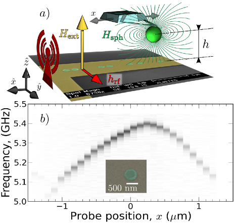
Figure 1: a) Schematic of the f-MRFM setup: an Fe sphere glued at the apex of a soft cantilever is scanned laterally above different pairs of Fe-V disks excited by a microwave field. b) Density plot of the f-MRFM signal as a function of the displacement $x$ of the sphere above an isolated disk. The inset is a SEM image of the $2R=600$ nm Fe-V disk (green) placed below the microwave antenna (gold).

The magnetic material used for this study is a $t=26.7$ nm thick Fe-V (10% V) film grown by molecular beam epitaxy on MgO(001) bonell09 ; mitsuzuka12 . This is a ferromagnetic alloy with a very high magnetization, $4\pi M_{s}=1.7\times 10^{4}$ G, and a very low magnetic Gilbert damping, $\alpha=2\times 10^{-3}$. The film is patterned into disks by e-beam lithography and ion milling techniques. The geometrical pattern (image in FIG.1a) consists in three pairs of nearby disks having the same nominal diameter $2R=600$ nm but different edge to edge separation: $s=200$ nm, 400 nm and 800 nm. Each set is separated by 3 $\mu$m in order to avoid cross coupling. An isolated disk of identical diameter is also patterned for reference purpose. The sample is then placed in the room temperature bore of an axial superconducting magnet. The disks are perpendicularly magnetized ($z$-axis) by an external field of 1.72 Tesla angle . This field is sufficient to saturate all the disks. A linearly polarized ($y$-axis) microwave field $h_{\text{rf}}$ is produced by a broadband Au strip-line antenna of width 5 $\mu$m deposited on top of a 50 nm thick Si₃O₂ isolating layer, above the magnetic disks. The f-MRFM experiment consists in detecting the mechanical motion produced by the magnetization dynamics in the Fe-V nano-disks of a Biolever cantilever with an Fe nano-sphere of diameter 700 nm glued at its apex (see FIG.1a) klein08 . We will consider in the following that the stray field of the tip $\bm{H}_{\text{sph}}$ reduces to the dipolar field created by a punctual magnetic moment $m_{\text{sph}}=3\times 10^{-10}$ emu placed at the center of the sphere. The role of the magnetic tip in f-MRFM is to create a field gradient tensor ${\widehat{\bm{G}}}=\nabla\bm{H}_{\text{sph}}$ on the sample in order to spatially code the resonance frequency and to provide a local detection lee10 .

These two features are illustrated by FIG.1b, which shows the dependence of the f-MRFM signal measured above the isolated disk as a function of the position of the tip on the $x$-axis. It displays the behavior of the lowest energy SW mode, where all spins are precessing in phase at the Larmor frequency around the unit vector ${\hat{\bm{z}}}$. The cantilever is scanned at constant height $h$ above the sample surface. The position $x=0$ corresponds to placing the probe on the axis of the disk.

We first concentrate on the variation of the FMR resonance frequency as a function of the $x$-position of the sphere. It displays a bell curve, whose shape is due to the additional bias field produced by the tip

$$\omega(x)=\omega_{\text{FMR}}+\gamma\{{H}_{\text{sph,z}}(x)\}\,\,,$$ (1)

where the first term is the resonance frequency in the absence of the sphere and the second term is the gyromagnetic ratio $\gamma$ times the spatial average of the $z$-component of the stray field of the sphere over the disk volume. The curly bracket indicates that this average should be weighted by the spatial profile of the lowest energy SW mode Bessel . The maximum shift of frequency occurs close to $x=0$, where the additional field from the f-MRFM sphere is maximal asym . The slope of the wings is proportional to the lateral field gradient $G_{zx}$. For $h\gg 2R$, it is maximum at $x\simeq 0.39\,h$, where $h$ is the height between the sample surface and the sphere center. At this location, the gradient is about $G_{zx}\approx 2.7\,m_{\text{sph}}/h^{4}$. Since it is important to keep $h$ as large as possible for stability purpose, the optimal $h$ is reached when $\gamma G_{zx}R>\Omega$. For our settings, this occurs at $h=1.8$ $\mu$m, leading to slope of about $0.3$ GHz/$\mu$m. At this distance, the maximum stray field of the sphere is about 140 G, a small variation compared to the static perpendicular field of 1.72 T, ensuring that no significant deformation of the SW modes profile is induced klein08 .

We then turn to the variation of the amplitude of the f-MRFM signal as a function of the position of the sphere in FIG.1b. The force acting on the cantilever can be calculated as the vertical force exerted by the tip on the sample, $F_{z}=G_{zz}\Delta M_{z}$, where $\Delta M_{z}$ is the variation of the sample magnetization induced by the FMR resonance klein08 . The gradient $G_{zz}$ decays as the power $1/x^{5}$, for large lateral displacement $x$. This decay ensures a local detection. Experimentally, the signal decreases by one order of magnitude when the probe is displaced by 1.2 $\mu$m laterally.

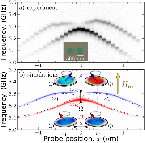
Figure 2: a) Density plot of the experimental f-MRFM spectra as a function of the displacement $x$ of the sphere above a pair of 600 nm Fe-V disks separated by $s=200$ nm. b) Predicted behavior by micromagnetic simulations. The upper mode (blue) corresponds to the anti-binding mode (A), while the lower (red) shows the binding mode (B). Insets: simulated precession profiles in each disk for modes (A) and (B) at the anti-crossing. The dashed lines would be the individual modes of each disks in the absence of dynamical coupling.

We now discuss the same experiment above the pair of two 600 nm disks separated by $s=200$ nm. The result is displayed on FIG.2a. Here $x=0$ corresponds to the middle of the pair. At each position $x$ of the f-MRFM probe, we can see two modes. The upper branch has two frequency maxima at $x_{1,2}=\mp 400$ nm, whose separation corresponds to the center to center distance between disk $1$ and disk $2$. The two maxima occur at slightly different frequencies, presumably due to a small difference in diameter between the two disks. When the probe is placed in between, $x_{1}<x<x_{2}$, the two levels anti-cross, which is a characteristic behavior of a coupled dynamics. Defining $\omega_{1,2}$ as the frequencies of the two uncoupled disks, the collective frequencies follow:

$$\omega_{A,B}=\frac{\omega_{1}+\omega_{2}}{2}\pm\sqrt{\left(\frac{\omega_{1}-\omega_{2}}{2}\right)^{2}+\left(\frac{\Omega}{2}\right)^{2}}$$ (2)

with ${\Omega}$ being the dynamical coupling strength. The two coupled eigen-frequencies $\omega_{A,B}$ correspond respectively to the anti-binding mode (A), where spins are precessing out-of-phase between the two disks, and to the binding mode (B), where spins are precessing in-phase naletov11 . In our f-MRFM experiment, $\omega_{1,2}$ both depend on $x$, see Eq.1: $\omega_{1,2}(x)=\omega_{\text{FMR}}+\gamma\{{H}_{\text{sph,z}}(x-x_{1,2})\}$. Using these dependencies in Eq.2, one can obtain an analytical expression for the frequency difference $\omega_{A}(x)-\omega_{B}(x)$ observed in FIG.2. At $x=0$, when $\omega_{1}=\omega_{2}$, the splitting $\omega_{A}-\omega_{B}$ exactly measures $\Omega$. Using this analytical expression for the spatial dependence of the splitting, we have fitted $\Omega/2\pi=50\pm 5$ MHz. We emphasize that this splitting is 2.5 times larger than the linewidth, found to be $20$ MHz. Theoretically, the coupling $\Omega$ for the magneto-dipolar interaction is defined by naletov11

$$\Omega^{2}=4\gamma^{2}h_{1,2}h_{2,1}\ .$$ (3)

$h_{i,j}$ represents the cross depolarization field produced by the SW in the $j$-th disk on the $i$-th disk ($i,j=1,2$) kostylev04 ; verba12 . It can be expressed as a function of the cross depolarization tensor elements, which have an analytical expression in the approximation of a uniform precession tandon04 : $h_{i,j}=2\pi M_{s}(\{N_{xx}^{i,j}\}+\{N_{yy}^{i,j}\})$. This formula reflects that the magneto-dipolar interaction is anisotropic and thus, it induces an elliptical precession in the two disks. For the separation $s=200$ nm, a numerical application yields $\{N_{xx}^{1,2}\}\approx-2\{N_{yy}^{1,2}\}\approx 0.0012$, which corresponds to a coupling field of about 10 G between the two disks, or a coupling frequency $\Omega/2\pi=56$ MHz, in very good agreement with the measured value.

Another striking feature in FIG.2a is the strong variation of the signal amplitude near the optimum coupling. We have explicitly plotted in FIG.3a the amplitude of the f-MRFM signal as a function of the lateral displacement $x$ of the probe, showing both the near extinction of the anti-binding mode (A) and the strong enhancement of the binding mode (B) near $x=0$. The ratio of hybridization in the two coupled disks follows the expression:

$$\left.\frac{c_{1}}{c_{2}}\right|_{A,B}=\left(\frac{(\omega_{1}-\omega_{2})\mp\sqrt{(\omega_{1}-\omega_{2})^{2}+\Omega^{2}}}{\Omega}\right)^{\mp 1}$$ (4)

Introducing the spatial dependence of $\omega_{1,2}$ described by Eq.1 in Eq.4 we can calculate the total force $F_{z}\propto P\left[c_{1}^{2}\,G_{zz}(x-x_{1})+c_{2}^{2}\,G_{zz}(x-x_{2})\right]$ acting on the cantilever. The power efficiency $P=|c_{1}+c_{2}|^{2}h_{\text{rf}}^{2}$ is proportional to the overlap integral between the uniform rf field and the collective SW mode (the vector sum of the transverse magnetization in the two disks) naletov11 . Using Eq.4, the dependence on $x$ of the force produced by the binding and anti-binding mode gives the continuous lines shown in FIG.3a. The difference between the two curves comes mainly from the selection rules defined in $P$. We find that at the optimum coupling (when $\omega_{1}$ and $\omega_{2}$ cross), the anti-binding mode (A) in Eq.4 has $c_{1}=-c_{2}$ , i.e., a precession with equal hybridization weight between the two disks and out-of-phase. The overlap with the uniform rf field excitation is thus zero at $x=0$, leading to a vanishing amplitude. In contrast, the binding mode (B) has $c_{1}=+c_{2}$ at the anti-crossing, i.e., a precession with equal hybridization weight too, but now in-phase between the two disks. It represents and enhancement of the absorbed power by a factor of $2^{2}$ compared to the amplitude in one disk.

We then study the effect the magneto-dipolar coupling on the linewidth of the collective mode. We observe that the linewidth does not change much with tuning and the observed variation with $x$ is below the 5% range. At the optimal tuning $x=0$, the linewidth measured is $\Delta f=22.3\pm 0.5$ MHz (see FIG.3b) and it becomes slightly larger $\Delta f=23.1\pm 0.5$ MHz at the maximum detuning $x=x_{1,2}$. For comparison we have displayed in FIG.3c the linewidth observed above the single disk, whose value $\Delta f=21.4\pm 0.5$ MHz. A small increase of the ratio $\Delta f/f$ is indeed expected for the dynamically coupled modes. This comes from the fact that this ratio is equal to $\Delta f/f=\alpha(H_{x}+H_{y})/\sqrt{H_{x}H_{y}}$, where $\alpha$ is the Gilbert damping, and $H_{x}$ and $H_{y}$ represent the two stiffness fields which characterize the torque exerted on the magnetization when it is tipped along the $x$- or $y$-axis gurevich96 . The degree of hybridization as well as the nature of the mode (A or B) change the values and signs of $H_{x}$ and $H_{y}$. For the binding mode, the magneto-dipolar coupling generates an elliptical precession whose long axis is along the two disks axis. The induced ellipticity $\mathcal{E}$ is maximum at the anti-crossing ($x=0$), with an amplitude $\mathcal{E}=\frac{\beta-1}{\beta+1}\frac{\Omega}{\omega_{B}}\approx 3\%$, with $\beta=\{N_{xx}^{1,2}\}/\{N_{yy}^{1,2}\}\approx-2$. An increase of ellipticity induces an increase of the linewdith, a behavior which is consistent with the small additional broadening measured in our experiment.

The analytical model used above to analyze the data assumes a uniform magnetization throughout the magnetic body. To take more precisely into account the 3D texture of the magnetization and the static deformation induced by the probe, we have also calculated the eigen-frequencies of the two lowest energy modes as a function of $x$ using SpinFlow3D, a finite element solver developed by In Silicio SpinFlow3D . The disks are discretized with a mesh size of 10 nm using a Delaunay mesh construction. At each position of the probe, we first calculate the equilibrium configuration in the disks. The Arnoldi algorithm is then used to compute the lowest eigen-values of the problem as well as the associated eigen-vectors. The result is represented in red and blue in FIG.2b for the two lowest energy modes. The precession patterns associated to each mode at the anti-crossing are shown in inset. In this color representation, the hue indicates the phase (or direction) of the oscillating magnetization, while the brightness indicates its amplitude. The simulation results confirm very nicely the interpretation made above in terms of amplitude and peak position.

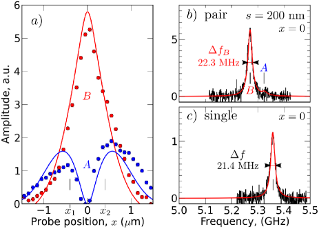
Figure 3: a) Variation of the amplitude of the binding (red) and anti-binding (blue) resonances as a function of the lateral position of the probe for the two disks separated by 200 nm. The solid lines correspond to the behavior following from Eq.4 (see text). b) Linewidth of the binding mode for the same pair at the tuning position ($x=0$) c) Comparison with the measurement of the linewidth above a single disk.

We have then repeated the same procedure on the two other pairs of disks, with larger edge to edge separation $s$. The strength of the dynamical coupling measured by f-MRFM is plotted as a function of $s$ in FIG.4. The main results is that, with our experimental parameters, $s$ needs to be less than the diameter of the disks in order to have $\Omega$ larger than the linewidth $\Delta f$. The data are plotted along with the analytical prediction (continuous line) and the simulations (dashed line with small dots). We observe an excellent overall agreement between the three sets of results, which all exhibit a similar decay with $s$ (not a simple polynomial law sukhostavets11 ). Still, the experimental points are systematically slightly below the theoretical expectation. This could be explained by the fact that the disks are slightly smaller than their nominal value (e.g., due to some oxidation at their periphery), or that the true separation between the disks is slightly larger than expected, which we have represented on the graph by the horizontal error bars. The agreement between the analytical model and the simulation is very good until $s=0.1$ $\mu$m. The discrepancy for very small $s$ is due to a significative change in the static magnetic texture. These changes are not taken into account by the analytical model. The effect of the static coupling is to produce a static magnetization along the $x$-direction. As shown by the simulations, this deformation enhances the strength of the dynamical coupling.

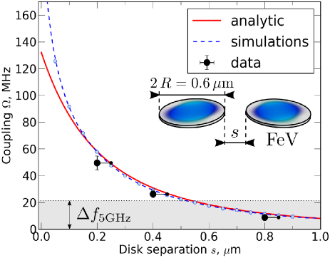
Figure 4: Coupling strength as a function of the separation $s$ between two disks. The plot compares the experimental findings to the predicted amplitude of the magneto-dipolar interaction either analytically (continuous line) or by micromagnetic simulations (small dots, dashed line is a guide to the eye).

In conclusion, we have shown that f-MRFM enables a detailed investigation of the dynamical dipolar coupling between two nearby magnetic objects, owing to the possibility of the technique to study both the tuned and detuned regime on the same object. It has been applied to study the collective SW dynamics in pairs nano-disks of Fe-V, an ultra-low damping material. Several signatures of the collective behavior have been experimentally evidenced and quantitatively explained: the anti-crossing, the hybridization of the modes and the effects on the linewidth. Moreover, we have found that in order to have a frequency splitting larger than the linewidth of the modes, the edge to edge separation between our disks has to be smaller than their diameter, due to the fast decay of the magneto-dipolar interaction. We believe that our method of local characterization of the dipolar coupling will be very useful to the field of magnonics.

This research work was partially supported by the French Grants VOICE ANR-09-NANO-006-01 and MARVEL ANR-2010-JCJC-0410-01.

References

- (1) K. W. Chou, A. Puzic, H. Stoll, G. Schütz, B. V. Waeyenberge, T. Tyliszczak, K. Rott, G. Reiss, H. Brückl, I. Neudecker, D. Weiss, and C. H. Back, J. Appl. Phys. 99, 08F305 (2006)
- (2) G. de Loubens, V. V. Naletov, M. Viret, O. Klein, H. Hurdequint, J. Ben Youssef, F. Boust, and N. Vukadinovic, J. Appl. Phys. 101, 09F514 (2007)
- (3) G. Gubbiotti, M. Madami, S. Tacchi, G. Carlotti, H. Tanigawa, and T. Ono, J. Phys. D: Appl. Phys. 41, 134023 (2008)
- (4) A. A. Awad, G. R. Aranda, D. Dieleman, K. Y. Guslienko, G. N. Kakazei, B. A. Ivanov, and F. G. Aliev, Appl. Phys. Lett. 97, 132501 (2010)
- (5) H. Jung, Y.-S. Yu, K.-S. Lee, M.-Y. Im, P. Fischer, L. Bocklage, A. Vogel, M. Bolte, G. Meier, and S.-K. Kim, Appl. Phys. Lett. 97, 222502 (2010)
- (6) A. Vogel, A. Drews, T. Kamionka, M. Bolte, and G. Meier, Phys. Rev. Lett. 105, 037201 (2010)
- (7) S. Sugimoto, Y. Fukuma, S. Kasai, T. Kimura, A. Barman, and Y. Otani, Phys. Rev. Lett. 106, 197203 (2011)
- (8) H. Ulrichs, V. E. Demidov, S. O. Demokritov, A. V. Ognev, M. E. Stebliy, L. A. Chebotkevich, and A. S. Samardak, Phys. Rev. B 83, 184403 (2011)
- (9) V. V. Kruglyak, P. S. Keatley, A. Neudert, R. J. Hicken, J. R. Childress, and J. A. Katine, Phys. Rev. Lett. 104, 027201 (2010)
- (10) A. D. Belanovsky, N. Locatelli, P. N. Skirdkov, F. A. Araujo, J. Grollier, K. A. Zvezdin, V. Cros, and A. K. Zvezdin, Phys. Rev. B 85, 100409 (2012)
- (11) V. V. Kruglyak, S. O. Demokritov, and D. Grundler, Journal of Physics D: Applied Physics 43, 264001 (2010)
- (12) A. D. Karenowska, J. F. Gregg, V. S. Tiberkevich, A. N. Slavin, A. V. Chumak, A. A. Serga, and B. Hillebrands, Phys. Rev. Lett. 108, 015505 (2012)
- (13) Y. Kubo, C. Grezes, A. Dewes, T. Umeda, J. Isoya, H. Sumiya, N. Morishita, H. Abe, S. Onoda, T. Ohshima, V. Jacques, A. Dréau, J.-F. Roch, I. Diniz, A. Auffeves, D. Vion, D. Esteve, and P. Bertet, Phys. Rev. Lett. 107, 220501 (2011)
- (14) F. Bonell, S. Andrieu, F. Bertran, P. Lefevre, A. Ibrahimi, E. Snoeck, C.-V. Tiusan, and F. Montaigne, IEEE Trans. Magn. 45, 3467 (2009)
- (15) K. Mitsuzuka, D. Lacour, M. Hehn, S. Andrieu, and F. Montaigne, Appl. Phys. Lett. 100, 192406 (2012)
- (16) In fact, the external field is tilted by in the -direction. Our setup does not allow in-situ adjustment of this small misalignment. Although it can be easily integrated in a complete analysis klein08 , this point will be neglected for the sake of simplicity as it brings minor correction.
- (17) O. Klein, G. de Loubens, V. V. Naletov, F. Boust, T. Guillet, H. Hurdequint, A. Leksikov, A. N. Slavin, V. S. Tiberkevich, and N. Vukadinovic, Phys. Rev. B 78, 144410 (2008)
- (18) I. Lee, Y. Obukhov, G. Xiang, A. Hauser, F. Yang, P. Banerjee, D. Pelekhov, and P. Hammel, Nature (London) 466, 845 (2010)
- (19) where is the area of the disk, is the -th order Bessel function and is its -th order root klein08 .
- (20) The asymmetries of the bell-shape curve (maximum of frequency shifted with respect to and to the maximum of amplitude, and different slopes in the wings) are due to the misalignment noted in angle .
- (21) V. V. Naletov, G. de Loubens, G. Albuquerque, S. Borlenghi, V. Cros, G. Faini, J. Grollier, H. Hurdequint, N. Locatelli, B. Pigeau, A. N. Slavin, V. S. Tiberkevich, C. Ulysse, T. Valet, and O. Klein, Phys. Rev. B 84, 224423 (2011)
- (22) M. P. Kostylev, A. A. Stashkevich, N. A. Sergeeva, and Y. Roussigné, J. Magn. Magn. Mater. 278, 397 (2004)
- (23) R. Verba, G. Melkov, V. Tiberkevich, and A. Slavin, Phys. Rev. B 85, 014427 (2012)
- (24) S. Tandon, M. Beleggia, Y. Zhu, and M. De Graef, J. Magn. Magn. Mater. 271, 9 (2004)
- (25) A. G. Gurevich and G. A. Melkov, Magnetization Oscillations and Waves (CRC Press, 1996)
- (26) http://www.insilicio.fr/pdf/Spinflow_3D.pdf
- (27) O. V. Sukhostavets, J. M. Gonzalez, and K. Y. Guslienko, Applied Physics Express 4, 065003 (2011)