More dynamical models of our Galaxy

Abstract

A companion paper presents an algorithm for estimating the actions of orbits in axisymmetric potentials. This algorithm is fast enough for it to be feasible to fit automatically a parametrised distribution function to observational data for the solar neighbourhood. We explore the predictive power of these models and the extent to which global models are constrained by data confined to the solar cylinder. We adopt a gravitational potential that is generated by three discs (gas and both thin and thick stellar discs), a bulge and a dark halo, and fit the thin-disc component of the distribution function to the solar-neighbourhood velocity distribution from the Geneva-Copenhagen Survey. We find that the disc’s vertical density profile is in good agreement with data at $z{\,\mathrel{\mathchoice{\lower 2.9pt\vbox{\halign{$\m@th\displaystyle\hfil#\hfil$\cr<\crcr\sim\crcr}}}{\lower 2.9pt\vbox{\halign{$\m@th\textstyle\hfil#\hfil$\cr<\crcr\sim\crcr}}}{\lower 2.9pt\vbox{\halign{$\m@th\scriptstyle\hfil#\hfil$\cr<\crcr\sim\crcr}}}{\lower 2.9pt\vbox{\halign{$\m@th\scriptscriptstyle\hfil#\hfil$\cr<\crcr\sim\crcr}}}\,}}500\,{\rm pc}$. The thick-disc component of the distribution function is then used to extend the fit to data from Gilmore & Reid (1983) for $z{\,\mathrel{\mathchoice{\lower 2.9pt\vbox{\halign{$\m@th\displaystyle\hfil#\hfil$\cr<\crcr\sim\crcr}}}{\lower 2.9pt\vbox{\halign{$\m@th\textstyle\hfil#\hfil$\cr<\crcr\sim\crcr}}}{\lower 2.9pt\vbox{\halign{$\m@th\scriptstyle\hfil#\hfil$\cr<\crcr\sim\crcr}}}{\lower 2.9pt\vbox{\halign{$\m@th\scriptscriptstyle\hfil#\hfil$\cr<\crcr\sim\crcr}}}\,}}2.5\,{\rm kpc}$. The resulting model predicts excellent fits to the profile of the vertical velocity dispersion $\sigma_{z}(z)$ from the RAVE survey and to the distribution of $v_{\phi}$ velocity components at $|z|\sim 1\,{\rm kpc}$ from the SDSS survey. The ability of this model to predict successfully data that was not used in the fitting process suggests that the adopted gravitational potential (which is close to a maximum-disc potential) is close to the true one. We show that if another plausible potential is used, the predicted values of $\sigma_{z}$ are too large. The models imply that in contrast to the thin disc, the thick disc has to be hotter vertically than radially, a prediction that it will be possible to test in the near future. When the model parameters are adjusted in an unconstrained manner, there is a tendency to produce models that predict unexpected radial variations in quantities such as scale height. This finding suggests that to constrain these models adequately one needs data that extends significantly beyond the solar cylinder. The models presented in this paper might prove useful to the interpretation of data for external galaxies that has been taken with an integral field unit.

1 Introduction

Large-scale surveys of our Galaxy are underway and in 2013 the European Space Agency will launch a satellite, Gaia, that is tasked with determining astrometry and photometry of unprecedented precision for a billion stars and gathering the spectra of a hundred million stars. The large outlays required to gather these data have been motivated by the expectation that we will be able to infer from the data not only the distribution of the Galaxy’s dark matter, but also quite detailed knowledge of the manner of its formation and its evolutionary history. Dynamical models of the Galaxy will be central to achieving these goals.

The simplest plausible dynamical models approximate the Galaxy by an axisymmetric body and exploit Jeans’ theorem to make the distribution function (df) dependent on just three isolating integrals. There are substantial advantages in identifying these integrals with the actions $J_{r}$, which quantifies a star’s radial oscillations, $J_{z}$, which quantifies oscillations perpendicular to the Galaxy’s equatorial plane, and $L_{z}$, the component of angular momentum about the assumed symmetry axis.

It turns out that good fits to the available observational data can be obtained with models whose dfs are simple analytic functions of the actions (Binney, 2010, hereafter B10). Given such a df, the calculation of predictions that can be compared with data is greatly facilitated if it is easy to determine the actions ${\bf J}$ of a given phase-space point $({\bf x},{\bf v})$. Analytic expressions for ${\bf J}({\bf x},{\bf v})$ are not available for any realistic Galactic potential and one has to have recourse to approximate and numerical methods. In B10 and Binney & McMillan (2011) the observable properties of models were obtained from the ‘adiabatic approximation’ for actions. In a companion paper we show that an algorithm based on the proximity of Galactic potentials to Stäckel potentials yields more accurate estimates of actions for a wider class of orbits. Moreover, this algorithm can be implemented in a sufficiently streamlined way that the observables of $\sim 50$ models can be estimated per hour on a laptop, and it becomes relatively straightforward to search the space of possible dfs automatically rather than by hand, and heavily influenced by prior prejudice, as was done in B10.

The purpose of this paper is to present results obtained by such automatic searches. Our aim is to explore the extent to which the global structure of the Galaxy can be pinned down by restricted sets of data when we impose a particular functional form for the df. The data we consider are restricted to the solar cylinder and for the most part quite old, so the models we obtain are far from definitive. Surveys now in hand will shortly yield data with much better statistics that extend significantly beyond the solar cylinder, so now is not the time to seek definitive results. Rather it is the moment to explore possibilities and connections between different types of data, and these are the tasks addressed in this paper.

Section 2 we describes the adopted potentials and Section 3 gives the functional forms of the adopted distribution functions. Section 4 shows fits obtained to observational data using two potentials, which differ in the assumed values of the distance $R_{0}$ to the Galactic centre and the local circular speed $\Theta_{0}$. Section 5 demonstrates that the thick disc has to be hotter vertically than radially, and addresses a variety of issues that are raised by the models. Section 6 sums up and considers what should be done next in relation to both surveys of our Galaxy and of external galaxies. An Appendix explains how we evaluate the multiple integrals over velocity that extract observables from the df.

Table 1: Parameters of the potentials

	Potential I			Potential II
Disc	Thin	Thick	Gas	Thin	Thick	Gas
$\Sigma_{0}[\!\,{\rm M}_{\odot}\,{\rm kpc}^{-2}]$	1.02e9	1.14e6	7.30e7	7.68e8	2.01e8	1.16e8
$R_{\rm d}[\!\,{\rm kpc}]$	2.4	2.4	4.8	2.64	2.97	5.28
$z_{\rm d}[\!\,{\rm kpc}]$	0.36	1	0.04	0.3	0.9	0.04
$R_{\rm h}[\!\,{\rm kpc}]$	0	0	4.0	0	0	4
Spheroid	Dark	Stellar		Dark	Stellar
$\rho_{0}[\!\,{\rm M}_{\odot}\,{\rm kpc}^{-3}]$	1.26e9	7.56e8		1.32e7	9.49e10
$q$	0.8	0.6		1	0.5
$\gamma$	-2	1.8		1	0
$\beta$	2.21	1.8		3	1.8
$r_{0}[\!\,{\rm kpc}]$	1.09	1		16.47	0.075
$r_{\rm cut}[\!\,{\rm kpc}]$	1000	1.9		100000	2.1

2 Gravitational potentials

We have worked with two gravitational potentials of the type presented by Dehnen & Binney (1998). Each potential is generated by three superposed discs: one representing the gas layer, one the thin disc and one representing the thick disc. The density of each disc is given by

$$\rho(R,z)={\Sigma_{0}\over 2z_{\rm d}}\exp\left[-\left({R_{\rm h}\over R}+{R\over R_{\rm d}}+{|z|\over z_{\rm d}}\right)\right],$$ (1)

where a non-zero value of $R_{\rm h}$ generates a central depression in an otherwise double-exponential disc. For each disc Table 1 gives the values taken by the parameters that appear in this formula. Spheroids representing the bulge and the dark halo also contribute to the potentials. The density of each spheroid is given by

$$\rho(R,z)={\rho_{0}\over m^{\gamma}(1+m)^{\beta-\gamma}}\exp\left[-(mr_{0}/r_{\rm cut})^{2}\right],$$ (2)

where

$$m(R,z)\equiv\sqrt{(R/r_{0})^{2}+(z/qr_{0})^{2}}.$$ (3)

Table 1 gives the values of the parameters for each spheroid. Potential I assumes $R_{0}=8\,{\rm kpc}$ and differs from Model 2 of Dehnen & Binney (1998) only in having the scale height of the thin disc increased from $z_{\rm d}=180\,{\rm pc}$ to $z_{\rm d}=350\,{\rm pc}$ and having the mass of the thin disc adjusted to increase the local circular speed from $\Theta_{0}=217\,{\rm km}\,{\rm s}^{-1}$ to $\Theta_{0}=220\,{\rm km}\,{\rm s}^{-1}$. This potential has a fairly short disc scale-length, so it is nearly a maximal-disc model. Potential II assumes $R_{0}=8.37\,{\rm kpc}$. It has been chosen to satisfy the constraints listed in McMillan (2011) and gives $\Theta_{0}=241\,{\rm km}\,{\rm s}^{-1}$.

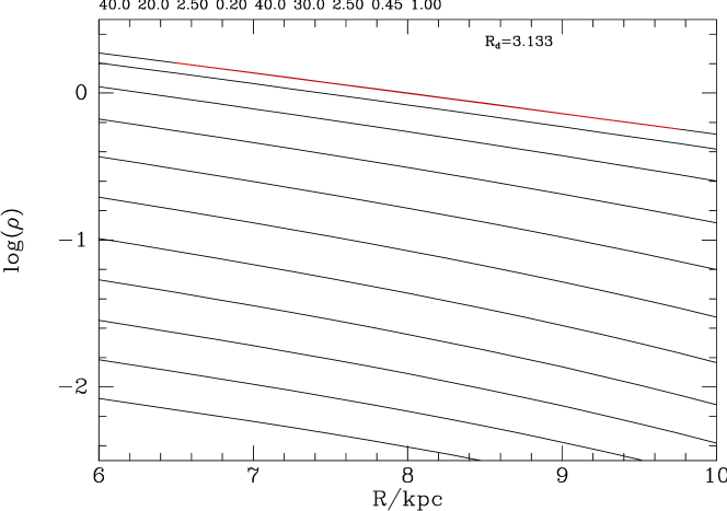
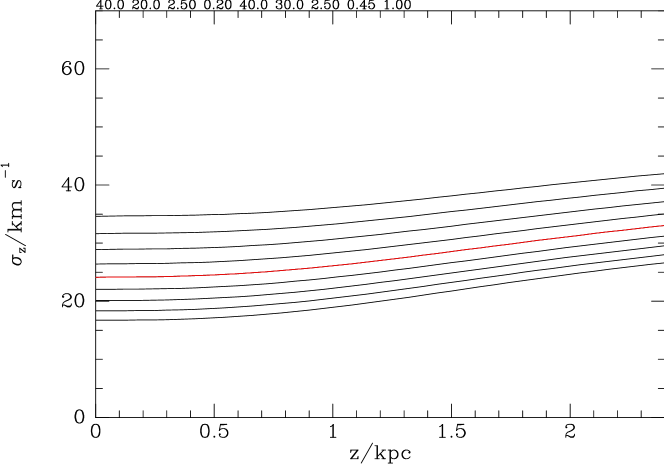
Figure 1: Properties of a quasi-isothermal component with $(\sigma_{r0},\sigma_{z0})=(40,20)\,{\rm km}\,{\rm s}^{-1}$, $R_{\rm d}=2.5\,{\rm kpc}$ and $q=0.45$. Top: density as a function of radius at heights $z$ that increase by $0.25\,{\rm kpc}$ from $z=0$ at the top. Bottom: vertical velocity dispersion as a function of $z$ at radii that from top to bottom increase from $6\,{\rm kpc}$ to $10\,{\rm kpc}$. In the top panel two points on the density profile in the plane are joined by a straight red line, and this line is an exponential with scalelength $R_{\rm d}=3.13\,{\rm kpc}$.

3 Distribution functions

Our dfs are built up out of “quasi-isothermal” components. The df of such a component is

$$f(J_{r},J_{z},L_{z})=f_{\sigma_{r}}(J_{r},L_{z})f_{\sigma_{z}}(J_{z},L_{z}),$$ (4)

where $f_{\sigma_{r}}$ and $f_{\sigma_{z}}$ are defined to be

$$f_{\sigma_{r}}(J_{r},L_{z})\equiv{\Omega\Sigma\over\pi\sigma_{r}^{2}\kappa}[1+\tanh(L_{z}/L_{0})]{\rm e}^{-\kappa J_{r}/\sigma_{r}^{2}}$$ (5)

and

$$f_{\sigma_{z}}(J_{z},L_{z})\equiv{\nu\over 2\pi\sigma_{z}^{2}}\,{\rm e}^{-\nu J_{z}/\sigma_{z}^{2}}.$$ (6)

Here $\Omega(L_{z})$, $\kappa(L_{z})$ and $\nu(L_{z})$ are the circular, radial and vertical epicycle frequencies respectively, while

$$\Sigma(L_{z})=\Sigma_{0}{\rm e}^{-R_{\rm c}/R_{\rm d}}$$ (7)

is the approximate surface density of the disc, with $R_{\rm c}(L_{z})$ the radius of the circular orbit with angular momentum $L_{z}$. The functions $\sigma_{r}(L_{z})$ and $\sigma_{z}(L_{z})$ control the radial and vertical velocity dispersions in the disc and are approximately equal to them at $R_{\rm c}$. Given that the scale heights of galactic discs do not vary strongly with radius (van der Kruit & Searle, 1981), these quantities must increase inwards. We adopt the following dependence on $L_{z}$:

$$\sigma_{r}(L_{z}) = \sigma_{r0}\,{\rm e}^{q(R_{0}-R_{\rm c})/R_{\rm d}}$$ (8)

$$\sigma_{z}(L_{z}) = \sigma_{z0}\,{\rm e}^{q(R_{0}-R_{\rm c})/R_{\rm d}},$$ (9)

which imply that the radial scale-length on which the velocity dispersions decline is $R_{\rm d}/q$. Our expectation is that $q\sim 0.5$.

In equation (5) the factor containing tanh serves to eliminate retrograde stars; the value of $L_{0}$ controls the radius within which significant numbers of retrograde stars are found, and should be no larger than the circular angular momentum at the half-light radius of the bulge. Provided this condition is satisfied, the results for the solar cylinder presented here are essentially independent of $L_{0}$.

Fig. 1 shows an example of a quasi-isothermal component. The upper panel shows that away from the plane its density is quite close to exponential in both $R$ and $z$ and the lower panel shows that the vertical velocity dispersion is independent of $z$ for $z{\,\mathrel{\mathchoice{\lower 2.9pt\vbox{\halign{$\m@th\displaystyle\hfil#\hfil$\cr<\crcr\sim\crcr}}}{\lower 2.9pt\vbox{\halign{$\m@th\textstyle\hfil#\hfil$\cr<\crcr\sim\crcr}}}{\lower 2.9pt\vbox{\halign{$\m@th\scriptstyle\hfil#\hfil$\cr<\crcr\sim\crcr}}}{\lower 2.9pt\vbox{\halign{$\m@th\scriptscriptstyle\hfil#\hfil$\cr<\crcr\sim\crcr}}}\,}}500\,{\rm pc}$.

 

 

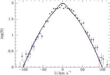
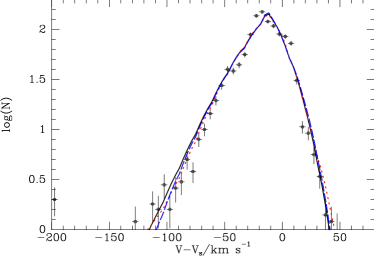
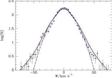
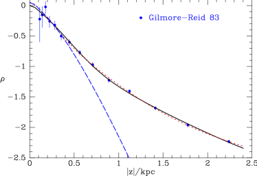
Figure 2: Fitting models in Potential I. The blue dashed curves show the result of choosing the parameters of the thin-disc df to optimise the fits of this model with no thick disc to the GCS velocity distributions of local stars shown in the first three panels. The full curves show the results obtained when a thick disc is included and the Gilmore-Reid points for the density shown in the bottom-right panel are included in the data to be fitted, without adjusting the previously-determined thin-disc df. The red dotted curves show the fits obtained when the parameters of both discs are simultaneously adjusted to optimise the fits to the GCS histograms and the Gilmore-Reid points. The parameters of the dfs responsible for the blue dashed, full and red-dashed curves are respectively listed in columns (a) to (c) of Table 2, respectively.

 

 

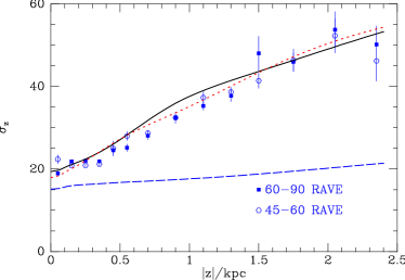
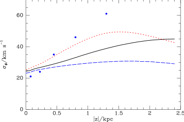
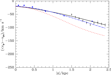
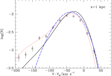
Figure 3: Prediction of the models fitted to to data as described in Fig. 2. The blue dashed curves are predictions for the model that has no thick disc, the full black curves are for the model obtained by adding a thick disc without adjusting the thin disc, and the red dotted curves show the model obtained by adjusting simultaneously both discs. Blue data points are from Burnett (2010) and black ones from Moni-Bidin et al. (2012). The model predictions for $\langle v_{\phi}\rangle$ at $z=1\,{\rm kpc}$ have been convolved with a Gaussian of dispersion $19\,{\rm km}\,{\rm s}^{-1}$, which is the estimated error of the SDSS data shown from Ivezic et al. (2008).

The df defined by equation (5) is the planar “pseudo-isothermal” df of B10, while that defined by equation (6) differs from the vertical “pseudo-isothermal” in B10 only in the replacement in the exponential of the vertical frequency $\Omega_{z}({\bf J})$ by the vertical epicycle frequency $\nu(L_{z})$. This replacement is expedient because at large radii $r$, where the potential becomes quite nearly spherical, $J_{z}\to L-|L_{z}|$ so for an orbit with $J_{r}=0$ $J_{z}\sim v_{\rm c}r$, while $\Omega_{z}\to\Omega\sim v_{\rm c}/r$, so $\Omega_{z}J_{z}\to$ a constant. Consequently, B10’s df tends to a constant at large $J_{z}$ and fixed $L_{z}$, which is inappropriate.

The functions $f_{\sigma_{i}}$ satisfy the normalisation conditions

$$\int_{0}^{\infty}{\rm d}J_{r}\,f_{\sigma_{r}} = {\Omega\Sigma\over\pi\kappa^{2}}[1+\tanh(L_{z}/L_{0})]$$ (10)

$$\int_{0}^{\infty}{\rm d}J_{z}\,f_{\sigma_{z}} = {1\over 2\pi},$$ (11)

so

$$g(L_{z})\equiv\int{\rm d}J_{r}\int{\rm d}J_{z}\,f(J_{r},J_{z},L_{z}),$$ (12)

which is the number of stars per unit angular momentum, decreases as $\Sigma(L_{z})/\kappa(L_{z})$, so roughly exponentially.

We take the df of the thick disc to be a pseudo-isothermal. The thin disc is treated as a superposition of the cohorts of stars that have age $\tau$ for ages that vary from zero up to the age $\tau_{\rm max}\simeq 10\,{\rm Gyr}$ of the thin disc. We take the df of each such cohort to be a pseudo-isothermal with velocity-dispersion parameters $\sigma_{r}$ and $\sigma_{z}$ that depend on age as well as on $L_{z}$. Specifically, from Aumer & Binney (2009) we adopt

$$\sigma_{r}(L_{z},\tau) = \sigma_{r0}\left({\tau+\tau_{1}\over\tau_{\rm m}+\tau_{1}}\right)^{\beta}{\rm e}^{q(R_{0}-R_{\rm c})/R_{\rm d}}$$

$$\sigma_{z}(L_{z},\tau) = \sigma_{z0}\left({\tau+\tau_{1}\over\tau_{\rm m}+\tau_{1}}\right)^{\beta}{\rm e}^{q(R_{0}-R_{\rm c})/R_{\rm d}}.$$ (13)

Here $\sigma_{z0}$ is the approximate vertical velocity dispersion of local stars at age $\tau_{\rm m}\simeq 10\,{\rm Gyr}$, $\tau_{1}$ sets velocity dispersion at birth, and $\beta\simeq 0.33$ is an index that determines how the velocity dispersions grow with age. We further assume that the star-formation rate in the thin disc has decreased exponentially with time, with characteristic timescale $t_{0}$, so the thin-disc df is

$$f_{\rm thn}(J_{r},J_{z},L_{z})={\int_{0}^{\tau_{\rm m}}{\rm d}\tau\,{\rm e}^{\tau/t_{0}}f_{\sigma_{r}}(J_{r},L_{z})f_{\sigma_{z}}(J_{z},L_{z})\over t_{0}({\rm e}^{\tau_{\rm m}/t_{0}}-1)},$$ (14)

where $\sigma_{r}$ and $\sigma_{z}$ depend on $L_{z}$ and $\tau$ through equation (3). We set the normalising constant $\Sigma_{0}$ that appears in equation (7) to be the same for both discs and use for the complete df

$$f(J_{r},J_{z},L_{z})=f_{\rm thn}(J_{r},J_{z},L_{z})+Ff_{\rm thk}(J_{r},J_{z},L_{z}),$$ (15)

where $F$ is a parameter that controls the fraction of stars that belong to the thick disc.

The dfs of the thin and thick discs each involve four important parameters, $\sigma_{r0}$, $\sigma_{z0}$, $R_{\rm d}$ and $q$. The df of the thin disc involves three further parameters, $\tau_{1}$, $\tau_{\rm m}$ and $\beta$, but we shall not explore the impact of changing these here because we do not consider data that permit discrimination between stars of different ages. Therefore following Aumer & Binney (2009) we adopt throughout $\tau_{1}=0.01\,{\rm Gyr}$, $\tau_{\rm m}=10\,{\rm Gyr}$ and $\beta=0.33$.

We have used the amoeba routine of Press et al. (1994) to adjust nine parameters of the overall df: $\sigma_{r0}$, $\sigma_{z0}$, $R_{\rm d}$, and $q$ for the thick and the thin discs plus the relative weight $F$ of the thick and thin discs.

4 models

The procedure generally adopted was to have amoeba fit the df to the $U$, $V$ and $W$ histograms for solar-neighbourhood stars from the Geneva-Copenhagen survey (Nordström et al., 2004; Holmberg et al., 2007, hereafter GCS) using only a thin disc, and then to add a thick disc to the df and use its parameters to secure a fit to vertical density profile of F dwarfs inferred by Gilmore & Reid (1983). In a final step amoeba adjusted all nine parameters of the df simultaneously to polish the fit to the GCS histograms and the Gilmore-Reid points.

The histograms fitted at each stage were compiled using all GCS stars closer than $150\,{\rm pc}$ with a probability of a constant line-of-sight velocity $>0.3$. The $U$ and $W$ components have been shifted to the Local Standard of Rest frame using $U_{\odot}=11.1\,{\rm km}\,{\rm s}^{-1}$ and $W_{\odot}=7.25\,{\rm km}\,{\rm s}^{-1}$ from Schönrich et al. (2011). The $V$ components were heliocentric.

In the second and third stages of fitting, the quantity to be minimised is

$$\chi^{2}={\textstyle{1\over 2}}(\chi^{2}_{U}+\chi^{2}_{V}+\chi^{2}_{W})+3\chi^{2}_{\rho},$$ (16)

where each component, $\chi_{U}^{2}$ etc., is the mean-square ratio of the difference between model and data divided by the formal observational error, and the sum of $U,V,W$ terms is what was minimised in the first stage of fitting. The relative weighting of the velocity and density data is an arbitrary choice designed to ensure that the relatively small number of density data are taken seriously. The iterations stop when the fractional variation of $\chi^{2}$ across the simplex is $<10^{-4}$.

4.1 Fits in Potential I

Fig. 2 shows the fits obtained in Potential I. All three dfs provides similar fits to the histograms of $U$ and $V$, but the df without a thick disc (blue dashed lines) falls below the data at large $|W|$ and $z{\,\mathrel{\mathchoice{\lower 2.9pt\vbox{\halign{$\m@th\displaystyle\hfil#\hfil$\cr>\crcr\sim\crcr}}}{\lower 2.9pt\vbox{\halign{$\m@th\textstyle\hfil#\hfil$\cr>\crcr\sim\crcr}}}{\lower 2.9pt\vbox{\halign{$\m@th\scriptstyle\hfil#\hfil$\cr>\crcr\sim\crcr}}}{\lower 2.9pt\vbox{\halign{$\m@th\scriptscriptstyle\hfil#\hfil$\cr>\crcr\sim\crcr}}}\,}}500\,{\rm pc}$ as is to be expected. The other two dfs provide excellent fits to the data apart from minor discrepancies within the cores of the $U$ and $V$ distributions. These discrepancies probably reflect the impact on the GCS histograms of non-equilibrium structure that lies beyond the scope of the present models. In particular, asymmetries in the observed distributions of $U$ and $W$ components cannot be reproduced by an equilibrium model. The bottom two panels of Fig. 2 provides two indications that the Galaxy’s true potential does not differ greatly from Potential I. First even though the thin-disc-only df was fitted only to the velocity data, it does provide a reasonable fit to the Gilmore-Reid points in the region $z{\,\mathrel{\mathchoice{\lower 2.9pt\vbox{\halign{$\m@th\displaystyle\hfil#\hfil$\cr<\crcr\sim\crcr}}}{\lower 2.9pt\vbox{\halign{$\m@th\textstyle\hfil#\hfil$\cr<\crcr\sim\crcr}}}{\lower 2.9pt\vbox{\halign{$\m@th\scriptstyle\hfil#\hfil$\cr<\crcr\sim\crcr}}}{\lower 2.9pt\vbox{\halign{$\m@th\scriptscriptstyle\hfil#\hfil$\cr<\crcr\sim\crcr}}}\,}}500\,{\rm pc}$ dominated by the thin disc. Second, the other two dfs can simultaneously fit both the $W$ distribution and the Gilmore-Reid points – in an erroneous potential it should be possible to fit either of these datasets but not both simultaneously.

Fig. 3 compares the predictions of these dfs with data that were not used in the fitting process. Each df is shown by the same line type as in Fig. 2. The blue data points come from Burnett (2010), black ones come from Moni-Bidin et al. (2012) and the open points in the bottom-right panel for the $V$ distribution at $|z|=1\,{\rm kpc}$ come from Ivezic et al. (2008). The predictions of the dfs shown in the bottom-right panel have been convolved with a Gaussian distribution of dispersion $19\,{\rm km}\,{\rm s}^{-1}$, the observational uncertainty reported by Ivezic et al. (2008). Burnett’s blue data points are the fruit of a preliminary analysis of $\sim 200\,000$ stars in the RAVE survey, roughly half dwarfs and half giants. Error bars are not available for the measures of $\langle v_{\phi}\rangle$ and $\sigma_{\phi}$. The black data points from Moni-Bidin et al. are obtained from a sample of 412 red giants seen near the south Galactic pole. They are shown with the errors given by Moni-Bidin et al. (2012) but these are significantly too small (Sanders, 2012). The open data points of Ivezic et al. relate to a very large sample of dwarf stars in the Sloan Digital Sky Survey.

Rather than plotting $\langle v_{\phi}\rangle$ we plot this less the value in the model of the Sun’s azimuthal velocity $v_{\phi\rm s}=\Theta_{0}+V_{\rm s}$, and we compare with heliocentric values of $v_{\phi}$. This comparison is to first order insensitive to the uncertain peculiar azimuthal velocity of the Sun, $V_{\odot}\simeq 11.5\,{\rm km}\,{\rm s}^{-1}$ (Schönrich et al., 2011).

As the points from Ivezic et al. illustrate, the distribution in $v_{\phi}$ is expected to be very skew and cannot be accurately characterised by a mean and a dispersion, especially far from the plane. Moreover, our dfs are designed to provide only disc stars, and far from the plane halo stars will make non-negligible contributions to the velocity distributions, especially at small $v_{\phi}$. So rather than comparing the predicted and measured values of $\langle v_{\phi}\rangle$ and $\sigma_{\phi}$ at various heights, we should judge a model on how well it reproduces the complete $v_{\phi}$ distribution at several values of $z$, as is done in the bottom-right panel of Fig. 3.

In the top left panel of Fig. 3 we see that, as expected, the thin-disc-only model predicts a rather constant value of $\sigma_{z}$ that lies below the data at all $z$. By contrast both models with thick discs fit the data to an extent that is remarkable given that the data played no part in choosing these models. The ability of these models to predict the run of $\sigma_{z}(z)$ is a further indication that Potential I does not differ greatly from the Galaxy’s potential.

The bottom-right panel of Fig. 3 shows that the red dotted line provides a good fit to the $v_{\phi}$ distribution at $z\simeq 1\,{\rm kpc}$ from Ivezic et al. (2008) aside from predicting slightly too many stars at $v_{\phi}-V_{\rm s}{\,\mathrel{\mathchoice{\lower 2.9pt\vbox{\halign{$\m@th\displaystyle\hfil#\hfil$\cr<\crcr\sim\crcr}}}{\lower 2.9pt\vbox{\halign{$\m@th\textstyle\hfil#\hfil$\cr<\crcr\sim\crcr}}}{\lower 2.9pt\vbox{\halign{$\m@th\scriptstyle\hfil#\hfil$\cr<\crcr\sim\crcr}}}{\lower 2.9pt\vbox{\halign{$\m@th\scriptscriptstyle\hfil#\hfil$\cr<\crcr\sim\crcr}}}\,}}-100\,{\rm km}\,{\rm s}^{-1}$. This defect is unfortunate because on account of its neglect of the stellar halo, the model should undershoot the data in this region. The lower left panel of Fig. 3 shows that in this model $\langle v_{\phi}\rangle$ falls too rapidly with $|z|$, a result consistent with the excess of stars at $v_{\phi}-V_{\rm s}<-100\,{\rm km}\,{\rm s}^{-1}$ in the lower-right panel. The upper-right panel suggests that in all three models $\sigma_{\phi}$ rises too gradually with $|z|$. However, this suggestion is contradicted by the lower-right panel, which implies that at $z=1\,{\rm kpc}$ the value of $\sigma_{\phi}$ for the model shown by the red dotted curve exceeds that in the Galaxy. Indeed data points for $\sigma_{\phi}$ from red-clump stars in RAVE prove to lie systematically below Burnett’s values (Williams et al. in preparation), so it seems likely that the data points in the upper-right panel of Fig. 3 are biased to high values.

Overall, we conclude that although the df in which all parameters have been simultaneously adjusted (red dotted lines) gives a remarkably good account of data that was not involved in its choice, a more perfect account of the data would be given by a df that is intermediate between this df and the one determined by fixing the thin and thick discs independently (full curves).

One finds, not surprisingly, that models with higher $\sigma_{\phi}$ tend to have lower $\langle v_{\phi}\rangle$, and vice versa.

Columns (a) – (c) of Table 2 give the parameters of the dfs of the models shown in Figs 2 and 3. In column (a) we see that there is nothing remarkable about the parameters of the thin disc initially chosen. The bottom half of column (b) shows that the thick disc that was selected to complement this thin disc has a remarkably small value of $\sigma_{r0}$ ($25.8\,{\rm km}\,{\rm s}^{-1}$), and a remarkably large normalisation ($F=0.772$), which implies that $\sim 43$ per cent of all stars are in the thick disc. Column (c) shows that an effect of simultaneously adjusting all nine parameters of the df is to weaken the radial gradient of $\sigma_{r}$ in the thin disc ($q=0.29\to q=0.14$) and to increase the gradient of $\sigma_{r}$ in the thick disc ($q=0.52\to q=0.71$). Another surprising effect is to increase the normalisation of the thick disc to $F=1.4$, so now 58 per cent of all stars lie in the thick disc.

When considering multi-parameter models such as these one should ask how unique a given fit to data really is. An indication is given by column (d) of Table 2, which gives the parameters of the df obtained by dispensing with a preliminary fit of the thin disc to the GCS data and from the outset simultaneously adjusting all nine parameters to optimise the fit to the GCS velocity histograms and the Gilmore-Reid density points. This df provides a fit to the given data which is barely distinguishable from that provided by the df of column (c) (red dotted lines), and very similar predictions to those plotted in Fig. 3; the only significant difference is that with column (d) at $z=1\,{\rm kpc}$ $\langle v_{\phi}\rangle$ is predicted to be $\sim 7\,{\rm km}\,{\rm s}^{-1}$ higher and $\sigma_{\phi}$ a similar amount lower than with column (c). There are however quite significant differences in the dfs: the thin-disc scale length is $2.80\,{\rm kpc}$ in column (c) and $2.17\,{\rm kpc}$ in column (d), and in the thin disc of column (d) the radial gradient in $\sigma_{r}$ virtually vanishes. Conversely, the thick-disc scale length is $2.5\,{\rm kpc}$ in column (c) and $3.66\,{\rm kpc}$ in column (d) while the already steep radial gradient of $\sigma_{r}$ in the thick disc has steepened to $q=1.07$ in column (d) from $q=0.705$ in column (c). Notice that increases in $R_{\rm d}$ and $q$ tend to compensate, because they tend to hold constant the scale length $R_{\rm d}/q$ on which $\sigma_{r}$ decreases with $R$. Experience shows that when tasked with fitting any data for the solar cylinder amoeba tends to choose thick discs which have large values of both $R_{\rm d}$ and $q$. One suspects that such models are not very physical and would be excluded by observational data from outside the solar cylinder.

Table 2: Parameters of the df chosen by amoeba for Potential I. Column (a) shows the thin-disc df chosen to optimise the fits to just the GCS velocity distributions. Column (b) gives the parameters obtained when we add both a thick disc and data for $\rho(z)$. Column (c) shows the df chosen when amoeba is given the opportunity to adjust all parameters simultaneously, starting with the df of column (b). In Figs. 2 and 3 the df of column (a) gives rise to the blue dashed curves, that of column (b) to the full curves, and that of column (c) to the red dotted curves. Column (d) shows the result of optimising the complete df in a single step, using both the GCS data and the $\rho(z)$ from the outset. The parameters listed in columns (c) and (d) yield very similar predictions for all observables. The df specified by Column (e) was chosen by fixing the parameters of the thin disc at plausible values and then adjusting the thick-disc parameters to optimise the fit to $\rho(z)$ and the wings of the GCS histograms for $U$ and $W$. Fig. 6 shows that this df conflicts with constraints on the $v_{\phi}$ distribution, especially away from the plane.

		(a)	(b)	(c)	(d)	(e)
Thin	$\sigma_{r0}$	40.1	40.1	42.2	42.3	30
	$\sigma_{z0}$	25.6	25.6	19.5	20.3	20
	$R_{\rm d}$	2.58	2.58	2.80	2.17	2.5
	$q$	0.289	0.289	0.142	.040	0.450
Thick	$\sigma_{r0}$	-	25.8	25.2	26.3	39.6
	$\sigma_{z0}$	-	45.0	32.7	34.0	30.4
	$R_{\rm d}$	-	2.11	2.50	3.66	2.28
	$q$	-	0.522	0.705	1.068	0.524
	$F$	0	0.772	1.424	0.224	0.989
$\chi^{2}$		16.8	9.40	7.61	7.44	4.51

 

 

 

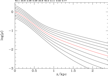
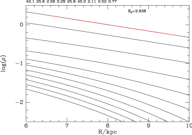
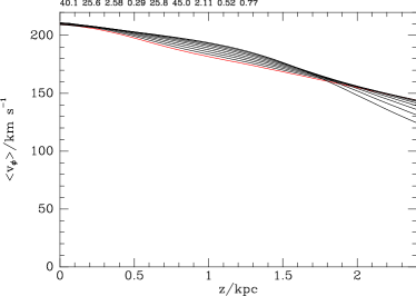
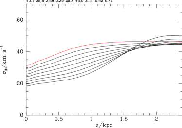
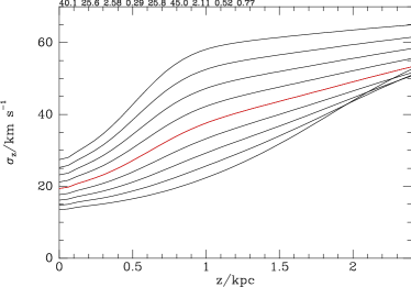
Figure 4: Global properties of the model generated by the df of Column (b) in Table 2 in Potential I. In the top left panel the curves show the density at constant $R$ with $R$ increasing from 6 to $10\,{\rm kpc}$ in steps of $0.5\,{\rm kpc}$ from top to bottom (the curve for $R=8\,{\rm kpc}$ is shown red), while the top right panel shows $\rho$ at fixed $|z|$, with $|z|$ increasing by $0.24\,{\rm kpc}$ from top to bottom. In the middle and bottom-left panels the curves are again for fixed values of $R$ from $6$ to $10\,{\rm kpc}$, but now with the curve for $R=6\,{\rm kpc}$ shown red. The bottom-right panel shows contours of constant density in the $(R,z)$ plane.

4.1.1 Large-scale structure predicted by the best DF

It is interesting to investigate the large-scale morphology of the disc produced by the df of column (b) of Table 2 since, as we have seen, this disc is consistent with most of the available data, which is essentially local in character. The upper panels of Fig. 4 show how $\rho(R,z)$ depends on $z$ at fixed $R$ (left) and on radius at fixed $|z|$ (right).

 

 

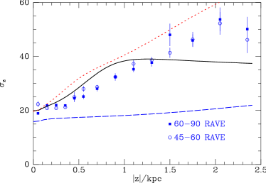
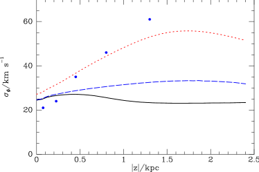
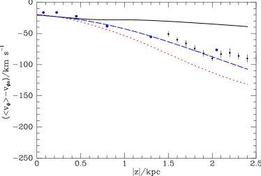
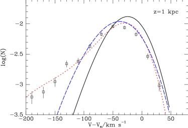
Figure 5: The predictions of dfs fitting in Potential II. The coding of the curves is as in Figs. 2 and 3: blue dashed curve a pure thin disc fitted to only the GCS velocity histograms; full black curves the result of using a thick disc to obtain a good fit to the Gilmore & Reid data for $\rho(z)$; red dotted curves the result of adjusting all nine parameters of the df simultaneously.

The top left panel shows that at both the smallest radii (top) and largest radii (bottom) the vertical density profile clearly comprises two straight-line segments, indicative of accurately exponential vertical density profiles for each disc. The height at which the thick disc becomes dominant shifts slowly upwards from $\sim 0.7\,{\rm kpc}$ at $R=6\,{\rm kpc}$ and the transition becomes less prominent with increasing radius as the scale-height of the thick disc decreases with increasing $R$. This decrease reflects the rather steep decline in $\sigma_{z0}$ implied by the scale-length $R_{\rm d}/q=3.24\,{\rm kpc}$. The scale-height of the thin disc slowly increases with radius.

In the top-right panel a red straight-line has been drawn between points at $R=6.5$ and $9.75\,{\rm kpc}$, and we see that in the plane the density profile is accurately exponential. The scale-length of this exponential is $R_{\rm d}=2.64\,{\rm kpc}$, slightly larger than the scale-length of the thin-disc’s df ($2.58\,{\rm kpc}$) and of the thin disc that generates the potential ($2.4\,{\rm kpc}$). As one moves away from the plane, the scale-length is constant in the region dominated by the thin disc, but at $z\sim 500\,{\rm pc}$ it begins to fall, reaching $1\,{\rm kpc}$ at $z=2.4\,{\rm kpc}$. This behaviour reflects the steep temperature gradient of the thick disc, which makes the density well above the plane fall rather slowly with $z$ at small $R$ and steeply with $z$ at large $R$.

Robin et al. (2003) fitted the 2MASS star counts to a model of the stellar density that had quite complex functional forms rather than simple double exponentials for the discs, but their model implies $R_{\rm d}\simeq 2.5\,{\rm kpc}$ for both the thin and thick discs and $z_{0}\simeq 0.8\,{\rm kpc}$ for the thick disc. Juric et al. (2008) infer from SDSS star counts that the thin disc has scale lengths $z_{0}=300\,{\rm pc}$ and $R_{\rm d}=2.6\,{\rm kpc}$, while the thick disc has $z_{0}=0.9\,{\rm kpc}$ and $R_{\rm d}=3.6\,{\rm kpc}$. Bovy et al. (2012) by contrast argue that the disc is a superposition of an infinite number of chemically homogeneous populations, with each population characterised by values of $z_{0}$ and $R_{\rm d}$ that vary from $(0.2,4.5)\,{\rm kpc}$ at the metal-rich extreme to $(1,2)\,{\rm kpc}$ at the metal-poor extreme. In particular, these two studies, both based on SDSS star counts, reach opposite conclusions regarding the ratio of the radial scale lengths of the thin and thick discs.

The middle panels of Fig. 4 show how the mean-streaming velocity (left) and $\sigma_{\phi}$ (right) vary with $z$. Again the red curves are for $R=6\,{\rm kpc}$. At $|z|<1\,{\rm kpc}$ the decline in $\langle{v}_{\phi}\rangle$ with $z$ is fastest at the smallest radii, but at greater heights $\langle{v}_{\phi}\rangle$ declines fastest with $z$ at the largest radii. At a given $z{\,\mathrel{\mathchoice{\lower 2.9pt\vbox{\halign{$\m@th\displaystyle\hfil#\hfil$\cr<\crcr\sim\crcr}}}{\lower 2.9pt\vbox{\halign{$\m@th\textstyle\hfil#\hfil$\cr<\crcr\sim\crcr}}}{\lower 2.9pt\vbox{\halign{$\m@th\scriptstyle\hfil#\hfil$\cr<\crcr\sim\crcr}}}{\lower 2.9pt\vbox{\halign{$\m@th\scriptscriptstyle\hfil#\hfil$\cr<\crcr\sim\crcr}}}\,}}1.5\,{\rm kpc}$, $\sigma_{\phi}$ is largest at small radii, but this is not true at $z\simeq 2\,{\rm kpc}$ because at large radii $\sigma_{\phi}$ starts to rise rapidly at $z\simeq 1\,{\rm kpc}$. In general $\sigma_{\phi}$ mirrors $\langle{v}_{\phi}\rangle$, rising as $\langle{v}_{\phi}\rangle$ falls.

The bottom-left panel of Fig. 4 shows that at $R=6\,{\rm kpc}$ (top curve) $\sigma_{z}$ rises most rapidly with $z$ for $z{\,\mathrel{\mathchoice{\lower 2.9pt\vbox{\halign{$\m@th\displaystyle\hfil#\hfil$\cr<\crcr\sim\crcr}}}{\lower 2.9pt\vbox{\halign{$\m@th\textstyle\hfil#\hfil$\cr<\crcr\sim\crcr}}}{\lower 2.9pt\vbox{\halign{$\m@th\scriptstyle\hfil#\hfil$\cr<\crcr\sim\crcr}}}{\lower 2.9pt\vbox{\halign{$\m@th\scriptscriptstyle\hfil#\hfil$\cr<\crcr\sim\crcr}}}\,}}0.9\,{\rm kpc}$, while at large $R$ the rise of $\sigma_{z}$ is gradual below $z\sim 0.8\,{\rm kpc}$ and then becomes rapid.

4.2 Fits in Potential II

We now briefly discuss results obtained by fitting dfs in Potential II, which is characterised by larger values of $R_{0}$ and the local circular speed $\Theta_{0}$. There are two reasons for turning to this potential. First, there are indications that $R_{0}>8\,{\rm kpc}$ and $\Theta_{0}{\,\mathrel{\mathchoice{\lower 2.9pt\vbox{\halign{$\m@th\displaystyle\hfil#\hfil$\cr>\crcr\sim\crcr}}}{\lower 2.9pt\vbox{\halign{$\m@th\textstyle\hfil#\hfil$\cr>\crcr\sim\crcr}}}{\lower 2.9pt\vbox{\halign{$\m@th\scriptstyle\hfil#\hfil$\cr>\crcr\sim\crcr}}}{\lower 2.9pt\vbox{\halign{$\m@th\scriptscriptstyle\hfil#\hfil$\cr>\crcr\sim\crcr}}}\,}}240\,{\rm km}\,{\rm s}^{-1}$ (e.g. McMillan & Binney, 2010), and second, Fig. 3 shows that dfs in Potential I cannot simultaneously make $\sigma_{\phi}$ and $\langle v_{\phi}\rangle$ as large as the (possibly suspect) data imply, and one might imagine this failure reflects inappropriate values of $R_{0}$ and $v_{\rm c}(R_{0})$. Table 3 gives the parameters of the dfs chosen by fitting to the the GCS velocity histograms and the Gilmore-Reid density values in three stages as before, and Fig. 5 shows the corresponding predictions.

Table 3: Parameters of the df chosen by amoeba for Potential II. Column (a) shows the thin-disc df chosen to optimise the fits to just the GCS velocity distributions. Column (b) gives the parameters obtained when we add both a thick disc and data for $\rho(z)$. Column (c) shows the df chosen when amoeba is given the opportunity to adjust all parameters simultaneously, starting with the df of column (b).

		(a)	(b)	(c)
Thin	$\sigma_{r0}$	40.9	40.9	42.3
	$\sigma_{z0}$	27.1	27.1	20.9
	$R_{\rm d}$	2.29	2.29	3.14
	$q$	0.239	0.239	0.246
Thick	$\sigma_{r0}$	-	28.2	28.3
	$\sigma_{z0}$	-	64.7	40.4
	$R_{\rm d}$	-	2.25	3.62
	$q$	-	0.283	1.070
	$F$	0	0.395	0.709
$\chi^{2}$		19.2	12.2	9.16

The second df in the sequence, whose predictions are shown by black full lines in Fig. 5, is less successful than the corresponding df in Potential I (Fig. 3) because it has too much rotation and too little random velocity; in Tables 2 and 3 this df is stands out for its exceptionally large value of $\sigma_{z0}=64.7\,{\rm km}\,{\rm s}^{-1}$ for the thick disc. When amoeba is allowed to adjust all the df’s parameters simultaneously, it increases the scale lengths of both discs from $\sim 2.3\,{\rm kpc}$ to $3.14$ and $3.62\,{\rm kpc}$ for the thin and thick discs, respectively, and reduces $\sigma_{z0}$ for both discs to $21$ and $40\,{\rm km}\,{\rm s}^{-1}$, respectively. The predictions of the final df are shown by the red dotted curves in Fig. 5. They are less successful than the corresponding predictions in Potential I in that the values of $\sigma_{z}$ are too large and the other predictions are only comparably successful. The excessive values of $\sigma_{z}$ suggest that Potential II has a disc that is too massive, and that a larger fraction of the mass that keeps $\Theta_{0}$ high at $8.37\,{\rm kpc}$ should reside in the dark halo.

 

 

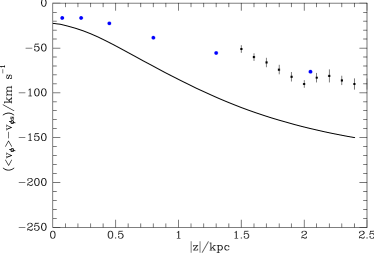
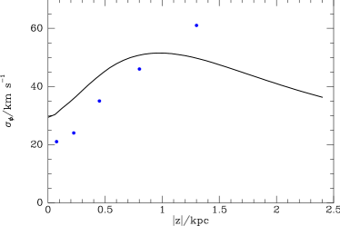
Figure 6: A model with a hot thick disc in Potential I. Column (e) of Table 2 lists the parameters of a df with a thick disc that is radially hotter than the thin disc. This df provides an excellent fits to the vertical density profile and the distribution of $W$ components of GCS stars, and a reasonable fit to $\sigma_{z}(z)$. However, it consistently fails to reproduce observations of the distribution of $v_{\phi}$ components because at large $z$ it places too many stars on highly eccentric orbits.

5 Discussion

An aspect of the fitting process that is troubling is that using only a thin disc amoeba is able to fit the wings as well as the cores of the $U$ and $V$ distributions of local stars – one would have expected the wings of these distributions to be filled out by the thick disc, just as is the case for the $W$ distribution. A consequence of this filling of the wings in $U$ and $V$ by the thin disc is that the thick discs subsequently fitted have unexpectedly small radial velocity-dispersion parameters, and these discs invariably have significantly larger vertical dispersions than radial ones.

Fig. 6 shows the result of attempting to remedy this situation by fixing the parameters of the thin-disc df to those listed in column (e) of Table 2 and then asking amoeba to choose the thick-disc parameters that minimise the residuals between the model and (i) the Gilmore-Reid points for $\rho(z)$, (ii) the GCS counts at $|U|>30\,{\rm km}\,{\rm s}^{-1}$ and (iii) the GCS counts at $|W|>20\,{\rm km}\,{\rm s}^{-1}$. The chosen df provides perfect fits to $\rho(z)$ and $N(W)$. The fit to $N(U)$ is good at $|U|{\,\mathrel{\mathchoice{\lower 2.9pt\vbox{\halign{$\m@th\displaystyle\hfil#\hfil$\cr>\crcr\sim\crcr}}}{\lower 2.9pt\vbox{\halign{$\m@th\textstyle\hfil#\hfil$\cr>\crcr\sim\crcr}}}{\lower 2.9pt\vbox{\halign{$\m@th\scriptstyle\hfil#\hfil$\cr>\crcr\sim\crcr}}}{\lower 2.9pt\vbox{\halign{$\m@th\scriptscriptstyle\hfil#\hfil$\cr>\crcr\sim\crcr}}}\,}}30\,{\rm km}\,{\rm s}^{-1}$ but significantly too sharply peaked at $|U|{\,\mathrel{\mathchoice{\lower 2.9pt\vbox{\halign{$\m@th\displaystyle\hfil#\hfil$\cr<\crcr\sim\crcr}}}{\lower 2.9pt\vbox{\halign{$\m@th\textstyle\hfil#\hfil$\cr<\crcr\sim\crcr}}}{\lower 2.9pt\vbox{\halign{$\m@th\scriptstyle\hfil#\hfil$\cr<\crcr\sim\crcr}}}{\lower 2.9pt\vbox{\halign{$\m@th\scriptscriptstyle\hfil#\hfil$\cr<\crcr\sim\crcr}}}\,}}15\,{\rm km}\,{\rm s}^{-1}$. The fit to $\sigma_{z}(z)$ is excellent at $z{\,\mathrel{\mathchoice{\lower 2.9pt\vbox{\halign{$\m@th\displaystyle\hfil#\hfil$\cr<\crcr\sim\crcr}}}{\lower 2.9pt\vbox{\halign{$\m@th\textstyle\hfil#\hfil$\cr<\crcr\sim\crcr}}}{\lower 2.9pt\vbox{\halign{$\m@th\scriptstyle\hfil#\hfil$\cr<\crcr\sim\crcr}}}{\lower 2.9pt\vbox{\halign{$\m@th\scriptscriptstyle\hfil#\hfil$\cr<\crcr\sim\crcr}}}\,}}1.2\,{\rm kpc}$ but is slightly lower than the data indicate at greater heights. However, Fig. 6 shows that this model predicts too many stars with low $v_{\phi}$. The surplus of low-angular-momentum stars becomes more marked as one moves away from the plane, and is a clear consequence of the thick disc being too hot radially. This experiment forces us to the conclusion that the thick disc really is hotter vertically than horizontally, and is indeed radially cooler than the thin disc. Moreover, it implies that the ability of the thin-disc df to fit even the wings of the GCS $U$ and $V$ distributions does not arise from an incorrect choice for the thin-disc’s df’s dependence on $J_{r}$, but reflects the fact that these wings are populated by stars that do not stray far from the plane.

When amoeba is permitted to adjust all nine parameters of the combined df simultaneously, it achieves slightly better representations of the data for the solar cylinder by adopting dfs that have unexpected, even implausible, radial structure. In particular there is a systematic tendency to choose for the thick disc a large radial scale-length and a large (and compensating) value of the parameter $q$ that controls the radial gradient of velocity dispersion. It seems that although data for the solar cylinder do very strongly constrain the dfs of the individual discs, they do not suffice to prevent one disc being played off against the other in unphysical ways. It is likely that such trade-offs would be suppressed if we had data that spanned a wider radial range.

The ability to distinguish chemically several populations of stars is a crucial aspect of astronomy that has been neglected in this work. The division of the disc into thin and thick components acquires objective meaning only when it is possible to distinguish stars of the two discs by age or metallicity (e.g. Binney & Merrifield, 1998, §10.4.3). The present models seem to require that the radial and azimuthal velocity dispersion of the population of $\alpha$-enhanced (and thus thick-disc) stars is smaller than its vertical velocity dispersion. This is a prediction that can be tested when large samples of photometrically selected stars with known abundances become available.

Whatever the outcome of this test, each chemically distinguishable population has an independent df, and the requirement that different populations co-exist within a common gravitational potential will surely provide the strongest constraints on the Galaxy’s mass distribution. Consequently, it is important to extend our formulae for the df to include chemical properties such as [Fe/H] and [$\alpha$/H]. We hope to present such extensions shortly.

Once one recognises that the Galaxy contains stars that span a range of age and chemistry, one has to engage with the differing propensities of stars to be picked up in a given survey. Some surveys select stars kinematically, some by colour and all select by apparent magnitude, so to predict from a df the numbers of stars of each species predicted in a given survey, one has to fold predictions of type presented here through a code such as Galaxia (Sharma et al., 2011) that produces number counts from phase-space distributions. We hope soon to present results obtained in this way.

We do not quote errors on the parameters of our models for two reasons. First amoeba merely seeks the minimum of a function, and determining the errors on the nine parameters and their correlations would involve a computational effort comparable to that involved in locating the minimum. Second, the formal errors are of little interest because the uncertainties in the parameters are not determined by the statistical errors, in the data, which are for the most part small, but by systematics, such as the existence of substructure that cannot be represented by the models. In fact, the values of $\chi^{2}$ per degree of freedom are quite large ($\sim 2$) so formally the models are inconsistent with the data.

Integral-field units now make it possible to map the line-of-sight velocity distribution and some chemical information across large parts of the images of external galaxies. Traditionally these data have been interpreted with either Schwarzschild models (Cappellari et al., 2007) or models based on the Jeans equations (Cappellari, 2008). These data could be interpreted with models similar to those presented here with greater ease than is possible with Schwarzschild models and greater rigour than the Jeans equations allow – the latter require an arbitrary closure assumption. This seems a fruitful direction for future work.

6 Conclusions

The simplest dynamical models of our Galaxy have distribution functions that are analytic functions of the action integrals of motion. We have fitted such dfs to measurements of the distribution of stellar velocities in the immediate neighbourhood of the Sun, and to these data in conjunction with an estimate of the vertical density profile at the solar circle. We have done this for two models of the Galaxy’s gravitational potential that differ in their values of $R_{0}$ and $\Theta_{0}$.

Using the potential with $R_{0}=8\,{\rm kpc}$ and $\Theta_{0}=220\,{\rm km}\,{\rm s}^{-1}$, the model optimised to fit only the local velocity distribution predicts a vertical density profile that fits the data below $\sim 0.5\,{\rm kpc}$ but falls increasingly below the data at greater distances from the plane. In fact it provides a good representation of the thin disc but deviates from the data where the thick disc is important because the local velocity distributions barely constrain the thick disc. When a thick disc is added and used to ensure that the density profile in the solar cylinder agrees with the measurements of Gilmore & Reid (1983), the model correctly (i) predicts a preliminary estimate of the run of vertical velocity dispersion with $z$ from the RAVE survey, (ii) fits two sets of measurements of $\langle{v}_{\phi}\rangle$ at $z<2.5\,{\rm kpc}$ and (iii) predicts the distribution of $V$ components of SDSS stars seen at $z\sim 1\,{\rm kpc}$. The single failure of this model is to predict values of $\sigma_{\phi}$ smaller than those obtained from preliminary analysis of RAVE data. If the adopted gravitational potential were significantly in error, it should not be possible to fit simultaneously the vertical profiles of $\rho$ and $\sigma_{z}$, so our findings suggest that the adopted potential is close to the truth.

When all nine parameters of the df are adjusted to refine the fits to the local velocity distributions and the vertical density profile, a model is obtained that predicts much better values of $\sigma_{\phi}$ at the price of predicting smaller values of $\langle{v}_{\phi}\rangle$ at $z{\,\mathrel{\mathchoice{\lower 2.9pt\vbox{\halign{$\m@th\displaystyle\hfil#\hfil$\cr>\crcr\sim\crcr}}}{\lower 2.9pt\vbox{\halign{$\m@th\textstyle\hfil#\hfil$\cr>\crcr\sim\crcr}}}{\lower 2.9pt\vbox{\halign{$\m@th\scriptstyle\hfil#\hfil$\cr>\crcr\sim\crcr}}}{\lower 2.9pt\vbox{\halign{$\m@th\scriptscriptstyle\hfil#\hfil$\cr>\crcr\sim\crcr}}}\,}}1\,{\rm kpc}$ than the raw data imply. After making allowance for observational error, the model does provide quite a good fit to the measured distribution of $v_{\phi}$ components at $z\simeq 1\,{\rm kpc}$.

When the same exercise is conducted with a potential in which $R_{0}=8.37\,{\rm kpc}$ and $\Theta_{0}=241\,{\rm km}\,{\rm s}^{-1}$, less satisfactory predictions are obtained. Most strikingly, in this potential $\sigma_{z}$ is predicted to be larger than the RAVE data imply, which suggests that this potential is generated by a disc that is more massive than the Galaxy’s disc.

At radii between $R=6\,{\rm kpc}$ and $R=10\,{\rm kpc}$ the favoured model’s vertical density profile is well approximated by two exponentials, a steep one associated with the thin disc and a much shallower thick-disc profile. These profiles meet at an altitude $\sim 0.7\,{\rm kpc}$. In this model the scale-height of the thin increases only slowly with radius, but that of the thick disc decreases with radius. Below $z\sim 0.9\,{\rm kpc}$ the mean-streaming velocity is similar at all radii and declines only slowly with increasing $z$, especially at large $R$. Above $z=0.9\,{\rm kpc}$ and at larger radii the mean-streaming velocity declines more rapidly with increasing $z$. A decline in mean-streaming velocity is always matched by an increase in azimuthal velocity dispersion.

A surprising, but apparently robust, prediction of these models is that, in contrast to the thin disc, the thick disc is hotter vertically than horizontally. When kinematically unbiased samples of stars with measured chemical compositions are available, it will be possible to test this prediction observationally.

A df of the type used here predicts many observables that we have not presented – for example the spatial distribution of stars of a given age or of the thick-disc stars, or the distributions of $U$ and $W$ components of velocity at $z\sim 1\,{\rm kpc}$ or any other altitude. We will release programs that calculate these predictions and it will be instructive to compare the predictions with further observations.

Appendix: Multiple integrals

Evaluation of a model’s observables, such as the density $\rho=\int{\rm d}^{3}{\bf v}\,f({\bf J})$ and velocity moments

$$\sigma_{ij}^{2}={1\over\rho}\int{\rm d}^{3}{\bf v}\,v_{i}v_{j}f({\bf J})$$ (17)

from its distribution function (df) $f({\bf J})$ involves many multiple integrals and it is important to do these efficiently. We do three-dimensional integrals with the aid of an oct-tree: the integral over a cubic region of volume $V$ is first estimated from values of the integrand $f$ at the corners and the centre of the cube as

$$I={\textstyle{1\over 2}}V[f(\hbox{centre})+{\textstyle{1\over 8}}\sum f(\hbox{corners})].$$ (18)

Then the integral is evaluated from the same formula applied to each of the eight sub-cubes into which the parent cube can be divided. If the sum of the sub-integrals differs by a given amount from the first estimate and the side-length of the sub-cubes exceeds a given length, the algorithm is run recursively on each of the sub-cubes. If either of these conditions is violated, the sum of the estimates for the sub-cubes is accepted as the value of the integral over the parent cube. For increased efficiency integrands for several moments of the df are evaluated simultaneously, with the criteria for exit based exclusively on the lowest moment. Analogous recursive algorithms are used to estimate one- and two-dimensional integrals.

References

- Abazajian (2009) Abazajian K., et al., 2009, ApJS, 182, 543-558
- Aumer & Binney (2009) Aumer M., Binney J., 2009, MNRAS, 397, 1286
- Binney (2010) Binney J., 2010, MNRAS, 401, 2318 (B10)
- Binney & McMillan (2011) Binney J., McMillan P.J., 2011, MNRAS, 413, 1889
- Binney & Merrifield (1998) Binney J., Merrifield M., 1998, “Galactic Astronomy”, Princeton University Press, Princeton
- Binney & Tremaine (1987) Binney J., Tremaine S., 1987, “Galactic Dynamics”, Princeton University Press, Princeton
- Bovy et al. (2012) Bovy J., Rix H.-W., Liu C., Hogg D.W., Beers T.C., Lee Y.S., 2012, ApJ, 753, 148
- Burnett (2010) Burnett, B., 2010, DPhil thesis, Oxford University
- Cappellari et al. (2007) Cappellari, M., et al., 2007, MNRAS, 379, 418
- Cappellari (2008) Cappellari, M., 2008, MNRAS, 390, 71
- Dehnen (1999) Dehnen W., 1999, AJ, 118, 1201
- Dehnen & Binney (1998) Dehnen W., Binney J., 1998, MNRAS, 298, 387
- Gilmore & Reid (1983) Gilmore G., Reid N., 1983, MNRAS, 202, 1025
- Holmberg et al. (2007) Holmberg J., Nordström B., Andersen J., 2007, A&A 475, 519
- Ivezic et al. (2008) Ivezic Z., Sesar B., Juric M., Munn J., 2008, ApJ, 684, 287
- Juric et al. (2008) Juric M., et al., 2008, ApJ, 673, 864
- McMillan (2011) McMillan P.J., 2011, MNRAS, 418, 1565
- McMillan & Binney (2010) McMillan P.J., Binney J., 2010, MNRAS, 402, 934
- Moni-Bidin et al. (2012) Moni-Bidin C., Carraro, G., Méndez, R.A., 2010, ApJ, 747, 101
- Nordström et al. (2004) Nordström B., Mayor M., Andersen J., Holmberg J., Pont F., Jørgensen B.R., Olsen E.H., Udry S., Mowlavi N., 2004, A&A, 418, 989
- Press et al. (1994) Press W.H., Teukolsky S.A., Vetterling W.T., Flannery B.P., 1994, Numerical Recipes in C, Cambridge: Cambridge University Press
- Robin et al. (2003) Robin, A.C., Reylé C., Derrière S., Picard S., 203, A&A 409, 523
- Sanders (2012) Sanders, J., 2012, MNRAS, in press
- Schönrich & Binney (2012) Schönrich R., Binney J., 2012, MNRAS, 419, 1546
- Schönrich et al. (2011) Schönrich R., Binney J., Dehnen W., 2012, MNRAS, 403, 1829
- Sharma et al. (2011) Sharma S., Bland-Hawthorn J., Johnston K.V., Binney J., 2011, ApJ, 730, 3
- Steinmetz et al. (2006) Steinmetz M. et al., 2006, AJ, 132, 1645
- van der Kruit & Searle (1981) van der Kruit P.C., Searle L., 1981, A&A, 95, 116