Spinons and Holons with Polarized Photons in a Nonlinear Waveguide

Abstract

We show that the spin-charge separation predicted for correlated fermions in one dimension, could be observed using polarized photons propagating in a nonlinear optical waveguide. Using coherent control techniques and employing a cold atom ensemble interacting with the photons, large nonlinearities in the single photon level can be achieved. We show that the latter can allow for the simulation of a strongly interacting gas, which is made of stationary dark-state polaritons of two species and then shown to form a Luttinger liquid of effective fermions for the right regime of interactions. The system can be tuned optically to the relevant regime where the spin-charge separation is expected to occur. The characteristic features of the separation as demonstrated in the different spin and charge densities and velocities can be efficiently detected via optical measurements of the emitted photons with current optical technologies.

1 Introduction

1.1 Spin-charge separation and quantum simulators

One-dimensional (1D) physical systems have attracted much attention due to their novel and sometimes spectacular features. Unlike two- or three-dimensional systems, the physics of 1D Lieb-Liniger model [1] is well captured by the Luttinger liquid theory in the low-energy domain [2]. In 1D Luttinger liquid theory, collective excitations rather than single excitations appear due to the tight transverse confinement forcing particles to move along one direction and thus converting any individual motion into a collective one. The collective modes of spin and charge in the 1D electronic gases surprisingly can be shown to propagate with different velocities, i.e., the spin and the charge separate into spinons and holons [2, 3, 4, 5]. In experiments, the observation of spin-charge separation is however challenging - the control of interactions is still elusive and no distinct features of separation are obtained, although several seminal works have been made using copper-oxide chain compounds SrCuO₂ [6], metallic chains [7], superconductors [8], and more recently, GaAs/AlGaAs heterostructures [9, 10, 11].

At the same time, works on artificially engineered quantum optical systems in which many-body effects could be reproduced in well controlled environments have recently emerged. To observe spin-charge separation in cold atoms, experimental proposals involving bosonic and fermionic species have been suggested [12, 13, 14, 15]. However, the challenges in the trapping and cooling of fermionic gases, especially the lack of necessary individual accessibility and measurement of correlations in general, make current results inconclusive. Strongly correlated photons and polaritons, as hybrid light-matter quantum simulators, have been recently proposed. Initially using coupled resonator implementations [16], Mott transitions [17, 18, 19] and then effective spin models and Fractional Hall states of light were shown to be possible [20, 21, 22, 23, 24, 25]. More recently, by employing hollow-core optical waveguides filled with cold atom ensembles and using slow-light techiques [26, 27, 28], it was shown that it is possible to prepare a Tonks gas of photons [29]. Using two atomic species, a two-component Lieb-Liniger model has also been recently suggested [30]. Compared to cold-atom proposals, photonic proposals should allow for more direct measurements of local observables and correlation functions of the emitted photon states.

In this article, we consider a novel scheme involving two oppositely circularly polarized quantum beams and single atomic species to simulate a two-component interacting gas in 1D. We note the difference to an earlier scheme, where two quantum fields with different frequencies interacting with two species of four-level atoms were employed [30]. The current proposal has the distinct advantage over in two major ways. Firstly in terms of more efficient detection of the correlation in output polarized states and secondly in terms of the loading and preparation process into the fiber which requires handling a single atomic species rather than two.

The paper is organized as follows. We first review the basics of the single- and two-component bosonic Lieb-Liniger model [1], and especially its mapping to Luttinger liquid theory. We then describe in detail the preparation of a polaritonic Lieb-Liniger model with two bosonic components in the waveguide employing slow-light techniques. Finally we discuss the necessary range of optical parameters in order to drive the system to the relevant spin-charge separation regime. We conclude by analyzing how the effective photonic spin and charge densities and velocities can be probed. This is done by releasing the trapped polaritons into outgoing photons where optical measurements can reconstruct the characteristic functions of the effect.

1.2 From Lieb-Liniger bosons to Luttinger liquids: The basics of Spin-Charge Separation revisited

One of the most famous 1D models is the Lieb-Liniger model [1], which describes $N$ bosons with a Dirac-delta interaction as

$$H^{\mathrm{s}}=-\frac{1}{2m}\sum_{i=1}^{N}\frac{\partial^{2}}{\partial z_{i}^{2}}+g\sum_{i<j=1}^{N}\delta\left(z_{i}-z_{j}\right),$$ (1)

where $m$ is the mass and $g$ is the interaction strength. Although the Lieb-Liniger model is exactly solvable through the Bethe ansatz approach, it is still generally very difficult to extract correlation functions from the solutions at any interaction regime. Luttinger liquid theory on the other hand can give the low energy universal description of the Lieb-Liniger model at low temperatures. In the Luttinger liquid phase, the low energy excitations are no longer single but collective modes with linear dispersion. The confinement of interactions between particles in 1D forces any individual motion to affect the collective system. The description of the dynamics in terms of collective bosonic fields is called ‘bosonization’ approach and we briefly present it in the following.

Assume $N$ particles described by $\psi(\mathbf{r})=\psi(z)\varphi_{0}(\mathbf{r}_{\perp})$, where the particles move along one direction, say $z$ direction. Strong confinement is applied to the transverse direction $\mathbf{r}_{\perp}=\{x,y\}$, allowing only for the lowest energy transverse quantum state $\varphi_{0}(\mathbf{r}_{\perp})$ to be considered. The Lieb-Liniger model of the parallel component reads [2, 3, 4, 5]

$$H^{\mathrm{s}}=\int dz[\frac{1}{2m}\partial_{z}\psi^{\dagger}\left(z\right)\partial_{z}\psi\left(z\right)+\frac{g}{2}\rho^{2}\left(z\right)],$$ (2)

where the collective bosonic fields $\psi\left(z\right)\$and $\psi^{\dagger}\left(z\right)$ can be expressed as

$$\psi\left(z\right)=e^{-i\theta\left(z\right)}\left[\rho\left(z\right)\right]^{1/2},\psi^{\dagger}\left(z\right)=\left[\rho\left(z\right)\right]^{1/2}e^{i\theta\left(z\right)},$$ (3)

with $\rho\left(z\right)=\psi^{\dagger}\psi$ the particle density and $\theta\left(z\right)$ the phase operator. As described in [2], the phase and density fields are canonically conjugated fields,

$$[\rho(z),e^{i\theta(z^{\prime})}]=\delta(z-z^{\prime})e^{i\theta(z^{\prime})},$$ (4)

and the collective density operator can be expressed as

$$\rho(z)=[\rho_{0}+\frac{1}{\pi}\partial_{z}\phi(z)]\sum_{m=-\infty}^{+\infty}\exp\{im[2\pi\rho_{0}z+2\phi(z)]\}.$$ (5)

If $\rho(z)$ varies slowly with z, we can retain the lowest frequency component for $m=0$ and write

$$\rho(z)\simeq\rho_{0}+\frac{1}{\pi}\partial_{z}\phi(z),$$ (6)

where the fields $\theta(z)$ and $\frac{1}{\pi}\partial_{z}\phi(z^{\prime})$ are canonically conjugated.

The Lieb-Liniger Hamiltonian (2) for the lowest component $\psi(z)\simeq e^{-i\theta\left(z\right)}\rho_{0}^{1/2}$ can be mapped to a Luttinger liquid with Hamiltonian (see [2, 3, 4, 5]):

$$H^{\mathrm{s}}=\int\frac{dz}{2\pi}[\upsilon K^{\mathrm{sl}}(\partial_{z}\theta)^{2}+\frac{\upsilon}{K^{\mathrm{sl}}}(\partial_{z}\phi)^{2}],$$ (7)

where all the interaction effects are encoded into two effective parameters: the propagation velocity of density disturbances $\upsilon$ and the so-called Luttinger parameter $K^{\mathrm{sl}}$ controlling the long-distance decay of correlations.

Going beyond the simple case with single-component bosonic system, interesting physics can be obtained by mixing two bosonic components or by considering two internal degrees of freedom of bosons, which is analogous to assigning a “spin”$1/2$ to bosons. The two-component Lieb-Liniger model in this case would read:

$$H^{\mathrm{t}}=\int dz\sum_{s=\uparrow,\downarrow}\left[\frac{1}{2m_{s}}\partial_{z}\psi_{s}^{\dagger}(z)\partial_{z}\psi_{s}(z)+\frac{\chi_{s}}{2}\rho_{s}^{2}(z)\right]+\int dz\chi_{\uparrow\downarrow}\rho_{\uparrow}(z)\rho_{\downarrow}(z),$$ (8)

where $m_{s}$ is the mass and $\chi_{s}$ and $\chi_{\uparrow\downarrow}$ are the intra- and interspecies interaction with $s=\uparrow$, $\downarrow$ representing the two spins. Following the literature [2, 3, 4, 5], the charge- and spin-related fields can be defined as:

$$\theta_{\mathrm{charge}}=\frac{\theta_{\uparrow}+\theta_{\downarrow}}{\sqrt{2}},\theta_{\mathrm{spin}}=\frac{\theta_{\uparrow}-\theta_{\downarrow}}{\sqrt{2}},\phi_{\mathrm{charge}}=\frac{\phi_{\uparrow}+\phi_{\downarrow}}{\sqrt{2}},\phi_{\mathrm{spin}}=\frac{\phi_{\uparrow}-\phi_{\downarrow}}{\sqrt{2}}.$$ (9)

The Hamiltonian separates into two parts (more details in [2]) and reads as: $H^{\mathrm{t}}=H_{\mathrm{charge}}+H_{\mathrm{spin}}$. The charge part is given by

$$H_{\mathrm{charge}}=\int\frac{dz}{2\pi}[u_{\mathrm{charge}}K_{\mathrm{charge}}(\partial_{x}\theta_{\mathrm{charge}})^{2}+\frac{u_{\mathrm{charge}}}{K_{\mathrm{charge}}}(\partial_{x}\phi_{\mathrm{charge}})^{2}]$$ (10)

and the spin part is defined as

$$H_{\mathrm{spin}} = \int\frac{dz}{2\pi}[u_{\mathrm{spin}}K_{\mathrm{spin}}(\partial_{x}\theta_{\mathrm{spin}})^{2}+\frac{u_{\mathrm{spin}}}{K_{\mathrm{spin}}}(\partial_{x}\phi_{\mathrm{spin}})^{2}]$$ (11)

$$+2\chi_{\uparrow\downarrow}\rho_{0}^{2}\cos\left(\sqrt{8}\phi_{\mathrm{spin}}\right)$$

under the separation conditions

$$\chi_{\uparrow}=\chi_{\downarrow},\frac{\rho_{0,\uparrow}}{m_{\uparrow}}=\frac{\rho_{0,\downarrow}}{m_{\downarrow}}.$$ (12)

Here $\rho_{0}=\rho_{0,\uparrow}+\rho_{0,\downarrow}$ and $\rho_{0,s}$ are the densities for two species. With $\chi=\chi_{s}$, $u=u_{s}=\sqrt{\rho_{0,s}\chi_{s}/m_{s}}$, and $K=K_{s}=\sqrt{\pi^{2}\rho_{0,s}/(m_{s}\chi_{s})}$, the charge and spin velocities and Luttinger parameters are $u_{\mathrm{charge,spin}}=u\sqrt{1\pm\chi_{\uparrow\downarrow}/\chi},$ $K_{\mathrm{charge,spin}}=K/\sqrt{1\pm\chi_{\uparrow\downarrow}/\chi}$.

2 Photonic Spin-Charge Separation in Nonlinear Optical Waveguides

2.1 The Optical Waveguide Setup

Our proposal is based on exploiting the available huge photonic nonlinearities possible to generate in specific quantum optical setups. More specifically, we envisage the use of a highly nonlinear waveguide where the necessary nonlinearity will emerge through the strong interaction of the propagating photons to existing emitters in the waveguide. Recent experiments have developed two similar setups in this direction, both capable of implementing our proposal with either current or near future platforms. In these experiments, cold atomic ensembles are brought close to the surface of a tapered fiber [31, 32] or are loaded inside the core of a hollow-core waveguide [33, 34, 35, 36] as shown in figure 1 (a). The available optical nonlinearity based on the Electromagnetically Induced Transparency (EIT) effect can be used as we will show to create situations where the trapped photons obey Lieb-Liniger physics.

The process to generate the strongly correlated states of photons is as follows: First, laser-cooled atoms exhibiting a multiple atomic-level structure shown in figure 1 (b) are moved into position so they will interact strongly with incident quantum light fields. Initially, resonant to the corresponding transitions, two optical pulses with opposite polarizations $\hat{E}_{\uparrow,+}(z,t)$ and $\hat{E}_{\downarrow,+}(z,t)$ are sent in from one direction, say the left side. They are injected into the waveguide with the co-propagating classical control fields $\Omega_{\uparrow,+}(t)$ and $\Omega_{\downarrow,+}(t)$ initially turned on. As soon as the two quantum pulses completely enter into the waveguide, the classical fields $\Omega_{s,+}$ are adiabatically turned off, converting $\hat{E}_{s,+}$ into coherent atomic excitations as in usual slow-light experiments for $s=\uparrow,\downarrow$. We then adiabatically switch on both $\Omega_{s,+}$ and $\Omega_{s,-}$ from two sides. The probe pulses become trapped due to the effective Bragg scattering from the stationary classical waves as analyzed in [26, 27, 28]. At this stage the pulses are noninteracting with the photons expanding freely due to the dispersion. By slowly shifting the $d$-levels, the effective masses can be kept constant whereas the effective intra- and interspecies repulsions are increased. This drives the system into a strongly interacting regime. This dynamic evolution is possible by keeping for example the corresponding photon detunings $\Delta_{s}$ constant while shifting the $d$-level. Once this correlated state is achieved, the fields - for example $\Omega_{s,+}$ - from the pair of control fields that trap polaritons, are slowly turned off. This will release the corresponding quasi-particles by turning them to propagating photons which will then exit the fiber. As all correlations established in the previous step are retained, these wave packets comprise of two separated effective charge and spin density waves.

2.2 Realizing a two-component Lieb-Liniger model of polarized photons

The system described above and shown in figure 1 obeys the Hamiltonian:

$$H^{\mathrm{o}} = -\int\sum_{s}n_{z}^{s}dz\{-\Delta_{s}\sigma_{b,s;b,s}-\sum_{s^{\prime}}\Delta_{ss^{\prime}}\sigma_{d,s,s^{\prime};d,s,s^{\prime}}^{\mathnormal{x}}$$ (13)

$$+\sqrt{2\pi}(g_{s}\sigma_{b,s;a}+\sum_{s^{\prime}}g_{ss^{\prime}}\sigma_{d,s,s^{\prime};c,s^{\prime}})$$

$$\times\left(\hat{E}_{s,+}\mathrm{e}^{\mathrm{i}k_{\mathrm{Q}\mathnormal{,s}}z}+\hat{E}_{s,-}\mathrm{e}^{-\mathrm{i}k_{\mathrm{Q}\mathnormal{,s}}z}\right)$$

$$+\left(\Omega_{s,+}\mathrm{e}^{\mathrm{i}k_{\mathrm{C}\mathnormal{,s}}z}+\Omega_{s,-}\mathrm{e}^{-\mathrm{i}k_{\mathrm{C}\mathnormal{,s}}z}\right)\sigma_{c,s;b,s}+\mathrm{h.c.}\},$$

where $s,s^{\prime}=\uparrow,\downarrow$ and $\left|d,\uparrow,\downarrow\right\rangle=\left|d,\downarrow,\uparrow\right\rangle$. The continuous collective atomic spin operators $\sigma_{\mu;\nu}\equiv\sigma_{\mu;\nu}(z,t)$ describe the averages of the flip operators $\left|\mu\right\rangle\left\langle\nu\right|$ over atoms in a small region around $z$. The density of atoms is $n_{z}^{\mathnormal{s}}$ and $g_{s}$, $g_{ss^{\prime}}$ are the coupling strengths between the quantum fields and atoms, while $\Delta_{s}$ and $\Delta_{ss^{\prime}}$ are one-photon detunings from the corresponding transitions. For simplicity, we assume that $g_{s}=g_{ss^{\prime}}=g$. Furthermore, we label the two quantum and two classical fields with frequencies $\omega_{\mathrm{Q}\mathnormal{,s}}$ and $\omega_{\mathrm{C}\mathnormal{,s}}$ and wave vectors $k_{\mathrm{Q}\mathnormal{,s}}$ and $k_{\mathrm{C}\mathnormal{,s}}$, respectively. Both quantum fields $\hat{E}_{\uparrow,+}(z,t)$ and $\hat{E}_{\downarrow,+}(z,t)$ drive four possible atomic transitions. The fields $\hat{E}_{s,\pm}(z,t)$ are detuned by $\Delta_{s}$ from the transition $|a\rangle\rightarrow|b,s\rangle$ and by $\Delta_{ss}$ from $|c,s\rangle\rightarrow|d,s,s\rangle$. $\hat{E}_{s,\pm}(z,t)$ also drive the transitions from $|c,s\rangle\rightarrow|d,s,\bar{s}\rangle$ with detuning $\Delta_{s\bar{s}}$. Here $\bar{s}=\uparrow,\downarrow$ and $\bar{s}\neq s$. Finally, the applied classical control beams with Rabi frequencies $\Omega_{s,\pm}(t)$ couple to both atoms and drive the transitions $|b,s\rangle\rightarrow|c,s\rangle$.

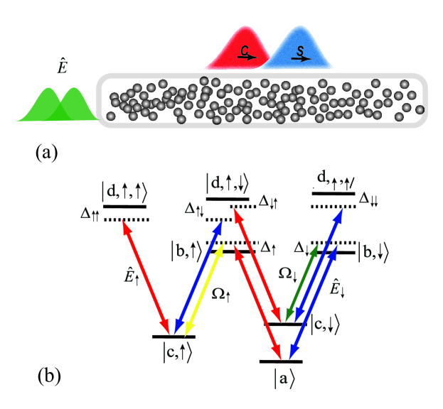
Figure 1: The model setup under consideration. In a nonlinear fiber ( a hollow core version is shown here but a tapered fiber approach could also be used), the cold atoms are interacting with two quantum light fields $\hat{E}_{s}$ (red and blue arrowlines) and two pairs of classical fields $\Omega_{s,\pm}$ (yellow and green arrowlines), where $\pm\$denotes the forward or backward propagation direction. The studied atomic level diagram and possible atomic transitions driven by two oppositely circularly polarized quantum pulses $\hat{E}_{s}$ and two control beams $\Omega_{s}$ is shown in (b). Appropriate tuning the couplings of light fields to the corresponding atomic transitions, forces the trapped polaritons to behave as an effective 1D quantum Luttinger liquid and reach the spin-charge separation regime. Coherently transferring the polaritons’ correlations to propagating light pulses and allowing them to exit the fiber, provide for the efficient measurement of both the dynamics of the propagation of the effective spin and charge quasiparticles and the effective spin and charge velocities characteristic of the effect taking place.

The evolution of the slowly-varying quantum operators $\hat{E}_{s,\pm}$ are given by four Maxwell-Bloch (MB) equations

$$\left(\partial_{t}+\nu\partial_{z}\right)\hat{E}_{s,\pm}=\mathrm{i}\sqrt{2\pi}n_{z}^{\mathnormal{s}}g\left(\sigma_{a;b,s,\pm}+\sigma_{c,s;d,s,s,\pm}+\sigma_{c,\bar{s};d,s,\bar{s},\pm}\right)$$ (14)

with four levels of the $s$-th atoms denoted as $|a,s\rangle$, $|b,s\rangle$ , $|c,s\rangle$ and $|d,s,s\rangle$. When writing down the MB equations (14), we have introduced the slowly-varying collective operators

$$\sigma_{\mu;\nu}=\sigma_{\mu;\nu,+}(z,t)\mathrm{e}^{\mathrm{i}k_{\mathrm{Q}\mathnormal{,s}}z}+\sigma_{\mu;\nu,-}(z,t)\mathrm{e}^{-\mathrm{i}k_{\mathrm{Q}\mathnormal{,s}}z},$$ (15)

and $\nu$ is the velocity of quantum fields in an empty waveguide . In the derivation of equations of motion we assume the Rabi frequencies of the control fields to be slowly varied. The slow-light polariton operators are defined as

$$\Psi_{s,\pm}=\cos\theta_{s}\hat{E}_{s,\pm}-\sin\theta_{s}\sqrt{2\pi n_{z}^{\mathnormal{s}}}\sigma_{c,s;a},$$ (16)

where $\tan\theta_{s}=g\sqrt{2\pi n_{z}^{\mathnormal{s}}}/\Omega_{s}$. For stationary polaritons we have assumed that the amplitudes of the counterpropagating classical fields are equal, i.e., $\Omega_{s,\pm}\equiv\Omega_{s}$. In the limit when the excitations are mostly in spin-wave form, i.e., $\sin\theta_{s}\simeq 1$, and since $\sigma_{c,s;a}=-g\hat{E}_{s,\pm}/\Omega_{s}$, the polariton operators become

$$\Psi_{s,\pm}=\sqrt{2\pi n_{z}^{\mathnormal{s}}}\frac{g}{\Omega_{s}}\hat{E}_{s,\pm}.$$ (17)

Setting $\Psi_{s}=(\Psi_{s,+}+\Psi_{s,-})/2$ and $A_{s}=(\Psi_{s,+}-\Psi_{s,-})/2$ as the symmetric and antisymmetric combinations of the two polaritons, we derive the equations of motion for the polariton combinations $\Psi_{s},\;A_{s}$:

$$\partial_{t}\Psi_{s} + \nu\partial_{z}A_{s}=-\pi\tan^{2}\theta_{s}\partial_{t}\Psi_{s}-\mathrm{i}\frac{2\pi g^{2}}{\Delta_{ss}}\left(2\Psi_{s}^{\dagger}\Psi_{s}+A_{s}^{\dagger}A_{s}\right)\Psi_{s}$$

$$-\mathrm{i}\frac{2\pi g^{2}}{\Delta_{s\bar{s}}}\left(2\Psi_{\bar{s}}^{\dagger}\Psi_{\bar{s}}+A_{\bar{s}}^{\dagger}A_{\bar{s}}\right)\Psi_{s}+\mathrm{noise},$$

$$\partial_{t}A_{s} + \nu\partial_{z}\Psi_{s}=-\mathrm{i}\frac{2\pi g^{2}}{\Delta_{s}}n_{z}^{\mathnormal{s}}A_{s}-\frac{2\pi g^{2}}{\Delta_{ss}}\Psi_{s}^{\dagger}\Psi_{s}A_{s}+\mathrm{noise}.$$ (18)

The noise terms in Eq. (18) account for the dissipative processes that take place during the evolution. Fortunately, for the dark-state polaritons under consideration, as long as the spontaneous emission rates $\Gamma$ from the states $|c,s\rangle$ and $|d,s,s^{\prime}\rangle$ are much less than the detunings $|\Delta_{ss^{\prime}}|$, the losses in the timescales of interest are not significant and thus can be neglected as discussed in [26, 27, 28, 29, 30]. Assuming optical depth of a few thousand and a large ratio between the density of atoms to the density of photons $n_{z}^{s}/n_{\mathrm{ph}}^{s}\sim 10^{4}$, the antisymmetric combinations $A_{\uparrow}$ and $A_{\downarrow}$ can be adiabatically eliminated from the equations of motion for the polaritons and moreover, the nonlinear terms like $\Psi_{s}^{\dagger}\Psi_{s}A_{s}$ and $A_{s}^{\dagger}A_{s}\Psi_{s}$ are negligible. In this regime, Eq. (18) simplifies to a nonlinear Schrödinger Eq. (19) for polaritons which reads:

$$i\partial_{t}\Psi_{s}=\frac{2\Delta_{s}\nu_{s}}{\Gamma_{\mathrm{1D}}^{s}n_{z}^{\mathnormal{s}}}\partial_{z}^{2}\Psi_{s}+\frac{\Gamma_{\mathrm{1D}}^{s}\nu_{s}}{\Delta_{ss}}\Psi_{s}^{\dagger}\Psi_{s}\Psi_{s}+\frac{\Gamma_{\mathrm{1D}}^{s}\nu_{s}}{\Delta_{s\bar{s}}}\Psi_{\bar{s}}^{\dagger}\Psi_{\bar{s}}\Psi_{s},$$ (19)

which is related to an effective two-component Lieb-Liniger model of polaritons

$$H=\int dz\sum_{s}\left[\frac{1}{2m_{s}}\partial_{z}\Psi_{s}^{\dagger}(z)\partial_{z}\Psi_{s}(z)+\frac{\chi_{s}}{2}\rho_{s}^{2}(z)\right]+\int dz\chi_{\uparrow\downarrow}\rho_{\uparrow}(z)\rho_{\downarrow}(z).$$ (20)

Here $m_{s}=-\Gamma_{\mathrm{1D}}^{s}n_{z}^{\mathnormal{s}}/(4\Delta_{s}\nu_{s})$ is the effective mass for $s$-th polaritons with $\Gamma_{\mathrm{1D}}^{s}=4\pi g^{2}/\nu$ the spontaneous emission rate of a single atom into the waveguide modes and $\nu_{s}=\nu\Omega_{s}^{2}/\left(\pi g^{2}n_{z}^{\mathnormal{s}}\right)$ the group velocity of the propagating polaritons. The intraspecies repulsion is characterized by $\chi_{s}=\Gamma_{\mathrm{1D}}^{s}\nu_{s}/\Delta_{ss}$ and the interspecies repulsion by $\chi_{\uparrow\downarrow}=\sum_{s=\uparrow,\downarrow}\Gamma_{\mathrm{1D}}^{s}\nu_{s}/\Delta_{s\bar{s}}$.

To reach the spin-charge separation regime, we employ the mapping to a Luttinger liquid model described in the previous section. For this to be possible, we should first of all check the tunability of the relevant parameters to the repulsive regime. This in our case (see Eq. (19)) implies tuning $\Delta_{s}\Delta_{ss}<0$ which leads to $m_{s}\chi_{s}>0$. Similarly $\Delta_{\uparrow}\Delta_{\downarrow}>0$ forces the effective masses $m_{\uparrow}m_{\downarrow}>0$ and $\Delta_{\uparrow\uparrow}\Delta_{\downarrow\downarrow}>0$ tunes $\chi_{\uparrow}\chi_{\downarrow}>0$. These conditions are satisfied by tuning the lasers such that: $\Delta_{\uparrow}$ and$\ \Delta_{\downarrow}$ are negative (positive) while at the same time $\Delta_{\uparrow\uparrow}$ and $\Delta_{\downarrow\downarrow}$ are positive (negative).

Apart from the repulsive interaction regime, the separation condition Eq. (12) needs to be satisfied as well, which in our case means setting:

$$\chi_{\uparrow}=\chi_{\downarrow},\frac{\rho_{0,\uparrow}}{m_{\uparrow}}=\frac{\rho_{0,\downarrow}}{m_{\downarrow}},$$ (21)

where the polariton density $\rho_{0,s}$ equals to the photon density $n_{\mathrm{ph}}^{s}$. The effective charge and spin densities are the sum and difference of the two-species polaritonic densities, which read as

$$\rho_{\mathrm{charge}}=\rho_{\uparrow}+\rho_{\downarrow},\rho_{\mathrm{spin}}=\rho_{\uparrow}-\rho_{\downarrow}$$ (22)

with $\rho_{s}=\left(\rho_{0,s}-\frac{1}{\pi}\nabla\phi_{s}\right)\sum_{m}\exp\left[i2m\left(\pi\rho_{0,s}z-\phi_{s}\right)\right]$. Keeping only the lowest components with $m=0,\pm 1$, the charge and spin density operators in the bosonic language can be represented as

$$\rho_{\mathrm{charge}} = \rho_{0}-\frac{\sqrt{2}}{\pi}\partial_{z}\phi_{\mathrm{charge}}+2\rho_{0}\cos\left[2k_{\mathrm{F}}z-\sqrt{2}\phi_{\mathrm{charge}}\right]\cos\sqrt{2}\phi_{\mathrm{spin}},$$ (23)

$$\rho_{\mathrm{spin}} = -\frac{\sqrt{2}}{\pi}\partial_{z}\phi_{\mathrm{spin}}+2\rho_{0}\sin\left[2k_{\mathrm{F}}z-\sqrt{2}\phi_{\mathrm{charge}}\right]\sin\sqrt{2}\phi_{\mathrm{spin}}.$$ (24)

Here the first term in $\rho_{\mathrm{charge}}$ is the average density $\rho_{0}=\rho_{0,\uparrow}+\rho_{0,\downarrow}$. In our two-species photonic system, we set $\rho_{0,\uparrow}=\rho_{0,\downarrow}=\frac{1}{2}\rho_{0}$ for each polarization component. The second gradient term in $\rho_{\mathrm{charge}}$ and $\rho_{\mathrm{spin}}$ are the density oscillations with zero momentum. The third term in $\rho_{\mathrm{charge}}$ and second term in $\rho_{\mathrm{spin}}$ are the density fluctuations of the $2k_{\mathrm{F}}$ components [37]. We label $\gamma_{s}$ as the ratio of the interaction to the kinetic energies for each polariton species $\gamma_{s}=m_{s}\chi_{s}/\rho_{0,s}$. Combining the two separation conditions in Eq. (21) together, one gets $\gamma_{\uparrow}=\gamma_{\downarrow}$. For $\chi=\chi_{s}$ and $\gamma=\gamma_{s}$, the velocities and Luttinger parameters can be expressed as $u=\chi/\sqrt{\gamma}$ and $K=\pi/\sqrt{\gamma}$. As also demonstrated for a similar system albeit with one quantum field [29], $\gamma$ here can also be tuned from zero to finite to extremely large, corresponding to non-, weak- and strong-correlated regimes, which implies a wide tunable range for $u$ and $K$.

2.3 Probing of the photonic spinons and holons

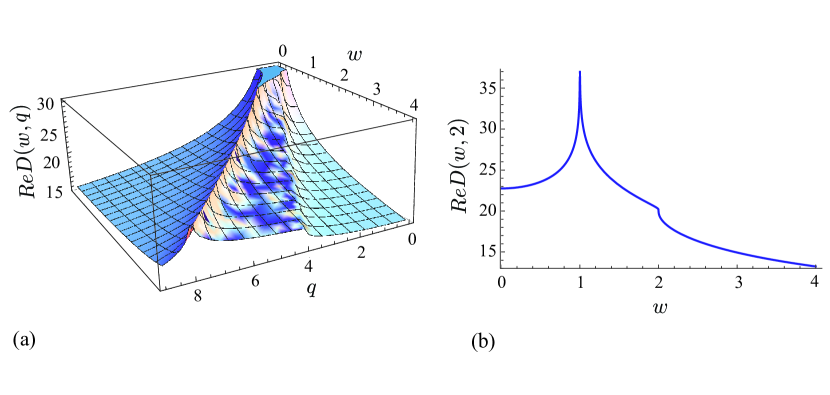
Figure 2: The Fourier transform of density-density correlations for our polaritonic system. It exhibits the characteristic splitting corresponding to the two different propagation velocities for the photonic spinons and holons, as calculated in [37]. The effective spin and charge velocities are $u_{\mathrm{charge}}=1$ and $u_{\mathrm{spin}}=0.5$ (normalized by $2\sqrt{\frac{2}{5}}u$), and the Luttinger parameters are $K_{\mathrm{charge}}=0.55$ and $K_{\mathrm{spin}}=1.1$. They translate in our case at optical depths of $OD=2000$, $10$ photons in each pulse initially, and single-atom co-operativity for each atomic species of $0.4$. In (b) a cut of the 3D plot at quasimomentum $q=2$ is plotted to show the distinct two peaks corresponding to the spin and charge velocities. The cross density-density correlations are experimentally reconstructed via typical optical measurements on the correlated photon states as they exit the fiber.

The typical detection of spin-charge separation can occur through dynamically probing the time evolution of a single excitation as in cold-atom proposals [12, 13, 14, 15], or by measuring the corresponding single-particle spectral function as in condensed matter experiments [2, 3, 4, 5, 6, 7, 8, 9, 10, 11]. In our case, we propose to extract the charge and spin velocities by measuring the Fourier transform of density-density correlations $D(\omega,q)$ for energy $\omega$ and momentum $q$. As derived for the two-component system in [37], for the $2k_{\mathrm{F}}$ component of density operator $\rho_{2k_{\mathrm{F}}}=2\rho_{0}\cos\left(2k_{\mathrm{F}}z-\sqrt{2}\phi_{\mathrm{charge}}\right)\cos\sqrt{2}\phi_{\mathrm{spin}}$ (the last term in Eq. (23)), the Fourier transform $D(\omega,q)$ of the density-density operator $\left\langle T_{\tau}\rho_{2k_{\mathrm{F}}}\left(z,\tau\right)\rho_{2k_{\mathrm{F}}}\left(0,0\right)\right\rangle$ is given by

$$D(\omega,q) = -\frac{4\pi\rho_{0}^{2}\left(\frac{\alpha}{2}\right)^{K_{\mathrm{charge}}+K_{\mathrm{spin}}}\Gamma\left(1-K_{\mathrm{charge}}/2-K_{\mathrm{spin}}/2\right)}{\Gamma\left(K_{\mathrm{charge}}/2+K_{\mathrm{spin}}/2\right)}$$ (25)

$$\times\left|\omega^{2}-u_{\mathrm{spin}}^{2}q^{2}\right|^{K_{\mathrm{charge}}/2+K_{\mathrm{spin}}/2-1}u_{\mathrm{spin}}^{1-K_{\mathrm{charge}}-K_{\mathrm{spin}}}$$

$$\times\exp\left[-i\pi\left(\frac{K_{\mathrm{charge}}+K_{\mathrm{spin}}}{2}-1\right)\Theta\left(\omega^{2}-u_{\mathrm{spin}}^{2}q^{2}\right)\right]$$

$$\times F_{1}\big{(}\frac{K_{\mathrm{charge}}}{2},\frac{K_{\mathrm{charge}}+K_{\mathrm{spin}}-1}{2},1-\frac{K_{\mathrm{charge}}+K_{\mathrm{spin}}}{2},$$

$$\frac{K_{\mathrm{charge}}+K_{\mathrm{spin}}}{2};1-\frac{u_{\mathrm{charge}}^{2}}{u_{\mathrm{spin}}^{2}},1-\frac{\omega^{2}-u_{\mathrm{charge}}^{2}q^{2}}{\omega^{2}-u_{\mathrm{spin}}^{2}q^{2}}\big{)},$$

where $\Gamma$ is the gamma function, $\Theta$ is the step function, $F_{1}$ is the Appell’s hypergeometric function, and $\alpha$ is a short-distance cutoff. $D(\omega,q)$ depends on the velocity $\omega/q$ and should exhibit two peaks centered around $u_{\mathrm{charge}}q$ and $u_{\mathrm{spin}}q$ [2, 3, 4, 5]. In our photonic system, probing of the spinon and holon branches can be done by measuring the correlation functions of densities of the fields as they exit, for a specific quasi-momenta $q$. For a clear distinction between the two effective spin and charge peaks, we should set our optical detectors around $q=2\pi/z_{0}$, i.e., $z_{0}$ apart ($z_{0}$ here corresponds to roughly the length of the fiber). To give an illustration of the expected behavior, $D(\omega,q)$ in the unit of $\rho_{0}^{2}\alpha$ is plotted in figure 2 with the intra- and interspecies repulsion ratio $\chi_{\uparrow\downarrow}/\chi=0.6$, which in turn tunes the charge and spin velocities to

$$u_{\mathrm{charge}}=2u_{\mathrm{spin}}=u\sqrt{1+\chi_{\uparrow\downarrow}/\chi}=2\sqrt{\frac{2}{5}}u,$$ (26)

and Luttinger parameters $K_{\mathrm{charge}}=\frac{1}{2}K_{\mathrm{spin}}=\frac{1}{2}\sqrt{\frac{5}{2}}K$. We choose $u_{\mathrm{charge}}=1$, $u_{\mathrm{spin}}=0.5$ and $K_{\mathrm{charge}}=0.55$, $K_{\mathrm{spin}}=1.1$ via tuning $u$ and $K$ wihch require $\gamma\sim 20$. This as shown in [29] is achieved at optical depths $OD=2000$ and roughly $N_{\mathnormal{ph}}^{\uparrow,\downarrow}=10$ photons initially in each pulse and single-atom co-operativity of $\eta=0.4$ . These values are for the moment out of the current experimental range where optical depths of a few hundred have been achieved, but should not be out of the question in the near to mid-term future [31, 32, 38]. In calculating the optical interaction parameters appearing in the Hamiltonian Eq. (20), we haven take into account both the linear and nonlinear loss mechanisms as layed out in [29].

3 Conclusion

We have described in detail a strongly correlated photonic scheme to simulate a purely fermionic effect, spin-charge separation. In more detail, we have shown that polarized photons interacting with a cold atomic ensemble can be made to obey two-component Lieb-Liniger physics and even behave as a quantum Luttinger liquid. The relevant interactions exhibit the necessary tunability for steering the photons to the effective spin-charge separation regime. Efficient observations of the characteristic features of the separation using standard quantum optical methods should be feasible based on correlations measurements of the outgoing photons which here carry opposite polarizations. The current proposal is different from a similar scheme proposed earlier by some of us, where two species of atoms were coupled to two quantum fields of two different frequencies but of same polarization [30]. Here a single species of atoms is shown to suffice in order to induce the required intra- and interspecies interactions, which combined with the easier detection of the polarized output states makes this approach more feasible.

4 Acknowledgments

We would like to acknowledge financial support by the National Research Foundation & Ministry of Education, Singapore.

References

References

• [1] Lieb E H and Liniger W 1963 Phys. Rev. 130 1605
• [2] Giamarchi T 2004 Quantum Physics in One Dimension (Oxford University Press, Oxford)
• [3] Girardeau M 1960 J. Math. Phys. 1 516-23
• [4] Girardeau M 1965 Phys. Rev. 139 B500
• [5] Paredes B et al 2004 Nature 429 277-81
• [6] Kim C et al 1996 Phys. Rev. Lett. 77 4054-7
• [7] Segovia P, Purdie D, Hengsberger M and Baer Y 1999 Nature 402 504-7
• [8] Lorenz T, Hofmann M, GrΓΌninger M, Freimuth A, Uhrig G S, Dumm M and Dressel M 2002 Nature 418 614-7
• [9] Auslaender O M et al 2005 Science 308 88-92
• [10] Kim B J et al 2006 Nat. Physics 2 397-401
• [11] Jompol Y et al 2009 Science 325 597-601
• [12] Recati A, Fedichev P O, Zwerger W and Zoller P 2003 Phys. Rev. Lett. 90 020401
• [13] Kecke L, Grabert H and Hausler W 2005 Phys. Rev. Lett. 94 176802
• [14] Kollath C, SchollwΓΆck U and Zwerger W 2005 Phys. Rev. Lett. 95 176401
• [15] Kleine A, Kollath C, McCulloch I P, Giamarchi T and SchollwΓΆck U 2008 Phys. Rev. A 77 013607
• [16] Angelakis D G, Santos M F, Yannopapas V and Ekert A 2007 Phys. Lett. A 362 377-80
• [17] Angelakis D G, Santos M F and Bose S 2007 Phys. Rev. A 76 031805(R)
• [18] Hartmann M J, BrandΓ£o F G S L and Plenio M B 2006 Nat. Phys. 2 849-55
• [19] Greentree A D, Tahan C, Cole J H and Hollenberg L C L 2006 Nat. Phys. 2 856-61
• [20] Rossini D and Fazio R 2007 Phys. Rev. Lett. 99 186401
• [21] Na N, Utsunomiya S, Tian L and Yamamoto Y 2008 Phys. Rev. A 77 031803(R)
• [22] Aichhorn M, Hohenadler M, Tahan C and Littlewood P B 2008 Phys. Rev. Lett. 100 216401
• [23] Gerace D, TΓΌreci H E, Imamoglu A, Giovannetti V and Fazio R 2009 Nat. Phys. 5 281-4
• [24] Carusotto I et al 2009 Phys. Rev. Lett. 103 033601
• [25] Angelakis D G, Bose S and Mancini S 2009 Eur. Phys. Lett. 85 20007
• [26] Fleischhauer M and Lukin M D 2000 Phys. Rev. Lett. 84 5094-7
• [27] Bajcsy M, Zibrov A S and Lukin M D 2003 Nature 426 638-41
• [28] Bajcsy M et al 2009 Phys. Rev. Lett. 102 203902
• [29] Chang D E et al 2008 Nat. Phys. 4 884-9
• [30] Angelakis D G, Huo M-X, Kyoseva E and Kwek L C 2011 Phys. Rev. Lett. 106 153601
• [31] Nayak K P et al 2007 Opt. Express 15 5431-8
• [32] Vetsch E, Reitz D, Sague G, Schmidt R, Dawkins S T, and Rauschenbeutel A 2010 Phys. Rev. Lett. 104 203603
• [33] Ghosh S, Sharping J E, Ouzounov D G and Gaeta A L 2005 Phys. Rev. Lett. 94 093902
• [34] Takekoshi T and Knize R J 2007 Phys. Rev. Lett. 98 210404
• [35] Christensen C A et al 2008 Phys. Rev. A 78 033429
• [36] Vorrath S, MΓΆller S A, Windpassinger P, Bongs K and Sengstock K 2010 New J. Phys. 12 123015
• [37] Iucci A, Fiete G A and Giamarch T 2007 Phys. Rev. B 75 205116
• [38] Bajcsy M et al 2011 Phys. Rev. A 83 063830