Dependence of the energy resolution of a scintillating crystal on the readout integration time.

Abstract

The possibilty of performing high-rate calorimetry with a slow scintillator crystal is studied. In this experimental situation, to avoid pulse pile-up, it can be necessary to base the energy measurement on only a fraction of the emitted light, thus spoiling the energy resolution. This effect was experimentally studied with a BGO crystal and a photomultiplier followed by an integrator, by measuring the maximum amplitude of the signals. The experimental data show that the energy resolution is exclusively due to the statistical fluctuations of the number of photoelectrons contributing to the maximum amplitude. When such number is small its fluctuations are even smaller than those predicted by Poisson statistics. These results were confirmed by a Monte Carlo simulation which allows to estimate, in a general case, the energy resolution, given the total number of photoelectrons, the scintillation time and the integration time.

1 Introduction

Electromagnetic calorimeters are often composed of inorganic scintillating crystals viewed by photodetectors. The energy resolution attainable depends primarily on the number of optical photons emitted by a scintillating crystal for a given energy deposit. Usually only a fraction of these photons are collected by a photodetector. In the following we consider a photomultiplier (PM), where the collected optical photons are converted in photoelectrons with an efficiency characteristic of the photocathode and amplified up to the anode by the dynode system.

Besides a possible non-linear crystal response [1], the anode charge pulse is therefore proportional to the energy deposited in the crystal by the primary particle and the fluctuations of this charge determine the energy resolution of the detector. The main contribution to this resolution comes from the statistics of the photoelectrons. In addition a small but not negligible contribution comes from the fluctuations in the PM gain and in particular from the gain of the first dynode. This resolution is worsened if the readout electronics integrates only part of the total charge delivered by the anode of the PM. This eventuality can occur when scintillating crystals with a long decay time are used in high-rate experiments where short integration times are needed.

In the present paper we will consider the possibility of using BGO crystals and PM’s for high rate experiments. In that case to limit the pile-up and the dead time, the PM pulses must be integrated over a time interval shorter than the scintillation time of the BGO ($\tau_{scint}=300$ ns). The deposited energy is then deduced from the maximum amplitude of the integrated pulse, measured by a peak-sensitive circuit. With this procedure only a fraction of the total charge is measured and a faster response is obtained at the cost of a worse resolution. This effect was experimentally studied for different integration times and the results were compared with a Monte Carlo (MC) simulation.

2 Experimental setup

The experimental setup is sketched in Fig. 1. Photons with an energy of 662 keV from a ¹³⁷Cs radioactive source are detected by a $2\times 2\times 18$ cm³ BGO crystal, read at both ends by two EMI-9814B PMs.

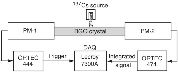
Figure 1: Experimental setup.

One of the two photomutipliers (PM-1) was used to trigger the acquisition of the pulses from the other photomultiplier (PM-2). In order to get rid of the noise, the trigger-signal from PM-1 was amplified and shaped with a gated biased amplifier (ORTEC-444) having an integration time of 250 ns. The signal from PM-2 was processed by a filter amplifier (ORTEC-474) that has a variable gain and an integration time ($\tau_{int}$) that can be set to 20, 50, 100, 200 and 500 ns. The output signal of that module was then acquired by a Lecroy WavePro 7300A digital oscilloscope, having a bandwidth of 300 MHz and a sampling rate of 250 MS/s.

3 Equivalent circuit

The ORTEC 474 integrating amplifier and its connection to the PM-2 anode can be represented by the equivalent circuit reported in Fig. 2.

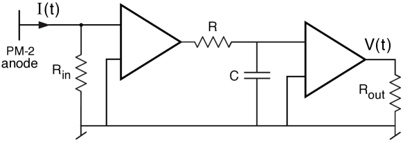
Figure 2: Equivalent circuit of the ORTEC-474 integrating amplifier. The two buffer amplifiers have an overall gain G while the integration time $\tau_{int}$ is equal to RC.

When a given energy is released in the crystal at the time $t=0$, the anode current delivered by PM-2 is:

$$I(t)=I_{0}\;e^{-t/\tau_{scint}}\times u(t)$$ (1)

where $\tau_{scint}$ is the decay time of the scintillator and $u(t)$ is the unit step function. The total charge per pulse released by the anode of PM-2 is $Q=I_{0}\;\tau_{scint}$. Using the standard Laplace transform method, the output signal $V(t)$ of the circuit on Fig. 2 turns out to be:

$$V(t)=\frac{G\;I_{0}\;R_{in}}{1-\alpha}\;(e^{-t/\tau_{scint}}-e^{-t/\tau_{int}})$$ (2)

where $R_{in}$ is the input resistance of the first buffer amplifier, $G$ is the overall gain, $\tau_{int}=RC$ is the integration time and $\alpha=\tau_{int}/\tau_{scint}$. For $N_{pe}\to\infty$, the maximum amplitude of the output signal is:

$$A_{N_{pe}\to\infty}=I_{0}\;R_{in}\;\alpha^{\;\;\alpha/(1-\;\alpha)}$$ (3)

which occurs at the time:

$$T_{N_{pe}\to\infty}=\tau_{int}\;\frac{ln\,\alpha}{\alpha-1}$$ (4)

From Eq. 2 the total charge ($Q_{out}$) of an output pulse is proportional to $Q$:

$$Q_{out}=\int_{0}^{\infty}\!\frac{V(t)}{R_{out}}\,dt=G\;I_{0}\;R_{in}\;\tau_{scint}=G\;R_{in}\;Q$$ (5)

4 Data taking

About 15000 pulses were recorded for each of the five possible values $\tau_{int}=$ 20, 50, 100, 200 and 500 ns. Each pulse was sampled every 4 ns during 10 $\mu$s and the resulting 2500 istantaneous amplitudes were acquired. A thousand pulses are shown in Fig. 3a, while in Fig. 3b the average waveform is reported for the five $\tau_{int}$ values.

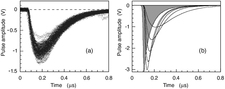
Figure 3: (a): A thousand of superimposed waveforms acquired with $\tau_{int}=$ 500 ns. (b): Waveforms obtained by averaging 15000 pulses: without integration (grey area not normalized) and with an integration time $\tau_{int}$ = 20, 50, 100, 200 and 500 ns respectively from the larger to the smaller signal.

To check the reproducibility of the results, four data-sets (A, B, C and D) were acquired under different conditions for all values of $\tau_{int}$.

• A and B were taken under the same conditions (HV of PM-2 equal to 1800 V and gain of the ORTEC-474 set to 10) but in different days in order to test the reproducibility of the results;

• C : HV of PM-2 equal to 1800 V and the ORTEC-474 gain set to 2;

• D : HV of PM-2 equal to 1750 V and the ORTEC-474 gain set to 10.

During the acquisition of the four data-sets the configuration on the trigger side of the set-up (PM-1 and ORTEC 444) was kept fixed. The trigger level of the oscilloscope was set sufficiently low to accept all the pulses from the 662 keV photons. The electronics noise was measured by acquiring data with a random triggers. The width of these noise spectra being 10 times smaller than that of the source signal, the contribution of the electronics noise to the energy resolution was neglected.

5 Data analysis

The acquired waveforms were analysed off-line. For each value of $\tau_{int}$ and for each pulse, the maximum amplitude ($A$), the peaking time ($T$) and the total charge ($Q_{out}$) were evaluated.

5.1 Total charge fluctuations

When the total charge of each pulse is measured, the energy resolution of the BGO crystal is mainly determined by the statistical fluctuations of the total number ($N_{pe}$) of the photoelectrons and by the fluctuations of the gain of the 12 PM dynodes ($g_{1},...,g_{12}$). Assuming a Poisson distribution for $N_{pe}$ and considering that in general $g_{1}\;>g_{2}\;=\;g_{3}\;=\;...\;=\;g_{12}\;\equiv\;g$ the energy resolution is given by [2, 3, 4, 5, 6]:

$$\frac{\sigma_{E}}{\overline{E}}=\frac{\sigma_{Q}}{\overline{Q}}=\frac{\sigma_{Q_{out}}}{\overline{Q}_{out}}=\frac{1}{\sqrt{\overline{N}_{pe}}}\;\sqrt{1+\frac{1}{\overline{g}_{1}}\left(\sum\limits_{i=0}^{k-1}\frac{1}{\overline{g}^{\;i}}\right)}\simeq\frac{1}{\sqrt{\overline{N}_{pe}}}\;\sqrt{1+\frac{1}{\overline{g}_{1}}\left(\frac{1}{1-1/g}\right)}$$ (6)

where $E$ is the measured energy and $k\;=\;12$ is the number of dynodes. Since $g$ is rather larger than 1, Eq.6 was approximated as:

$$\frac{\sigma_{E}}{\overline{E}}=\frac{\sigma_{Q}}{\overline{Q}}=\frac{\sigma_{Q_{out}}}{\overline{Q}_{out}}\simeq\frac{1}{\sqrt{\overline{N}_{pe}}}\;\sqrt{1+\frac{1}{\overline{g}_{1}}}$$ (7)

that is equivalent to take into account only the contribution of the fluctuations of the first dynode. In Fig. 4a a typical experimental spectrum of $Q_{out}$ is shown. Taking into account the HV of PM-2, the characteristics of the 9814B tube [7] and of the BeCu dynodes [2] the average gain of the first dynode was assumed to be $\overline{g}_{1}\simeq 6$.

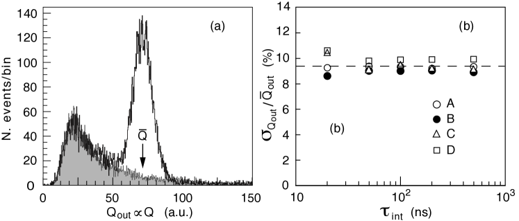
Figure 4: (a): A typical spectrum of the total pulse charge. The peak from 662 keV gammas is superimposed to a background (grey area) which was measured without the ¹³⁷Cs source. (b): Relative total charge resolution as a function of $\tau_{int}$ for the four sets (A, B, C and D) of data taking. The dashed line represents the expected behaviour for $\overline{N}_{pe}=130$. The statistical errors are within the points.

The energy resolution becomes:

$$\frac{\sigma_{E}}{\overline{E}}=\frac{\sigma_{Q_{out}}}{\overline{Q}_{out}}=\frac{1.08}{\sqrt{\overline{N}_{pe}}}$$ (8)

In Fig. 4b the experimantal values of $\sigma_{Q_{out}}/\overline{Q}_{out}$ are reported for the five values of $\tau_{int}$ and for the four sets of data taking. They show, as expected, a flat behaviour with respect to $\tau_{int}$. A constant fit to these data allows to determine from Eq. 8 the average number of photoelectrons $\overline{N}_{pe}=130^{+13}_{-11}$.

5.2 Maximum amplitude fluctuations

When the measurement of the total charge $Q$ takes too long, the energy deposited in the crystal can be inferred from the maximum amplitude $A$ of the integrated signal. In Fig. 5a a spectrum of $A$ obtained in the present test with $\tau_{int}=100$ ns is shown. The fluctuations ($\sigma_{A}$) on $A$ are obtained by a gaussian fit to the data. In Fig. 5b the experimental resolution $\sigma_{A}/\overline{A}$ is reported as a function of $\tau_{int}$. At large values of $\tau_{int}$ and in particular for $\tau_{int}\gg\tau_{scint}$, $\sigma_{A}/\overline{A}$ tends to the value of $\sigma_{Q_{out}}/\overline{Q}_{out}$, while at smaller values of $\tau_{int}$ the resolution worsen. To clarify the dependence of $\sigma A/A$ on $\tau_{int}$, a naive Poissonian model based on an extension of Eq. 8 was adopted. According to this model the resolution is given by:

$$\frac{\sigma_{E}}{\overline{E}}=\frac{\sigma_{A}}{\overline{A}}=\frac{1.08}{\sqrt{\overline{n}_{pe}}}$$ (9)

where $n_{pe}$ is the number of photoelectrons which contribute, for each event, to its maximum amplitude $A$, i.e. those emitted before the peaking time $T$ of that event.

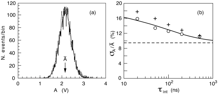
Figure 5: (a): Example of a spectrum of the maximum pulse amplitude A. The curve is a gaussian fit to the data. (b): Experimental maximum amplitude resolution (open points) as a function of $\tau_{int}$. The crosses are the values predicted by Eq.’s 9 and 11 with $\overline{N}_{pe}=130$ and with the measured values of $\overline{T}$ (Fig. 6). The statistical errors are within the points. The curve is the prediction of the MC (see Sec.6). The dashed line is the asymptotic value of the curve, which is equal to $\sigma_{Q_{out}}/\overline{Q}_{out}$.

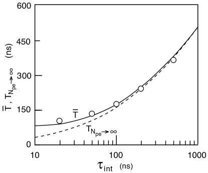
Figure 6: Experimental average peaking time ($\overline{T}$) for the five considerd values of $\tau_{int}$. The error bars are within the points. The continuous curve is the prediction of the MC (see Sec.6) for $\overline{N}_{pe}=130$. When $N_{pe}\to\infty$ the continuous curve tends to the dashed curve represented by Eq. 4.

The average value $\overline{n}_{pe}$ was approximated to the fraction $F$ of the average total number of photoelectron emitted before the experimentally measured values of $\overline{T}$:

$${\overline{n}_{pe}} =F\overline{N}_{pe}$$ (10)

$$F =(1-e^{-\overline{\vphantom{|^{.}}T}/\tau_{scint}})$$ (11)

In Fig. 6 the measured dependence of $\overline{\vphantom{|^{.}}T}$ on $\tau_{int}$ is reported.

In Fig. 5b the predictions of Eq.’s 9 and 11 are compared with the experimental results. While for $\tau_{int}=500$ ns the agreement is good, at lower values of $\tau_{int}$ the experimental resolution is better than predicted with the naive model. To understand this discrepancy, a detailed Monte Carlo simulation of the experimental situation was performed.

6 The Monte Carlo simulation

The formulae reported in Sec. 3 represent the response of an RC integrator excited by an exponentially decreasing current composed of a very large number of electrons, so that the charge quantization is washed out. In the situation we are considering, the average number of photoelectrons per pulse is relatively small so that the response of the device must be simulated with a MC. The input current $I(t)$ is described as a sum of delta functions, each one corresponding to an incoming photoelectron. Then the amplitude of the integrated pulse at a time $t$ turns out to be the sum of the contributions from all the photoelectrons emitted before that time:

$$V(t)=R_{in}\;(\frac{q}{\tau_{int}})\sum\limits_{i=1}^{n(\,t)}G_{i}\;e^{-(t-t_{i})/\tau_{int}}$$ (12)

where $q$ is the electron charge, $n(t)$ is the number of photoelectrons emitted before the time $t$, $t_{i}$ ($i=1,n$) is the emission time of the $i$-th electron ($0<t_{i}<t$) and $G_{i}$ is the PM gain for the $i$-th electron. The probability distribution function of the $t_{i}$ is a decreasing exponential with a decay time equal to $\tau_{scint}$. For a fixed $\;t$, $n(t)$ follows a Poisson distribution with a mean

$$\overline{n}(t)=\overline{N}_{pe}(1-e^{-t/\tau_{scint}})$$ (13)

It is worthwile to note that Eq. 12 represents a single pulse that can be used to measure the energy, only if there is an effective pile-up of the contributions of many photoelectrons belonging to the same detected particle. This occurs if the integration time $\tau_{int}$ is much larger than the average time interval between two consecutive photoelectrons ($\thickapprox\tau_{scint}/\overline{N}_{pe}$):

$$K\equiv\overline{N}_{pe}\frac{\tau_{int}}{\tau_{scint}}\gg 1$$ (14)

while if $K\lesssim 1$ the energy released in the scintillator gives rise only to a series of single photoelectron pulses. In the present experiment $K$ ranges from 8.7 (at $\tau_{int}=20$ ns) to 217 (at $\tau_{int}=500$ ns).

In the MC simulation all the aforementioned effects were taken into account. The MC was run with $10\leq\overline{N}_{pe}\leq 10^{4}$ and for $\tau_{int}$ ranging from 10 ns to 1 $\mu$s. For each of the $\sim 100$ pairs of values $(\overline{N}_{pe},\tau_{int})$ about 10000 pulses were generated. For each simulated pulse the MC calculates its amplitude $V(t)$ every ns during an interval of 2 $\mu$s. The maximum amplitude $A$ and the time $T$ at which this maximum occurs were recorded for each pulse and the relative fluctuations $\sigma_{A}/\overline{A}$ were determined.

6.1 Comparison with experimental data

For a comparison with the experimental data, the MC was run with $\overline{N}_{pe}=130$. The Poisson fluctuations of the gain $g$ of the first dynode, with a mean value $\overline{g}=6$, were also taken into account.

Figure 7: (a) A typical pulse generated by MC with $N_{pe}=130$ and $\tau_{int}=500$ ns. Each sharp discontinuity in the pulse shape corresponds to the arrival of a photoelectron. (b) Example of experimental pulse recorded with the same $\tau_{int}$.

In Fig. 7 a typical pulse generated by MC with $\tau_{int}=500$ ns is compared with an experimental pulse recorded with the same integration time. The agreement between the two shapes is quite good.

In Fig. 5b the dependence of $\sigma_{A}/\overline{A}$ and in Fig. 6 the mean value of the peaking time distribution ($\overline{T}$) on $\tau_{int}$, calculated with the MC, are compared with the experimental points. In both cases the agreement is quite good. This confirms that in the present experimental conditions the experimental resolution is better than predicted by the naive model based on a Poissonian statistcs. These checks give confidence in the MC simulation and allow to use it to predict, in the most general experimental situation, which is the energy resolution attainable with an integrator followed by a peak-sensitive electronics.

6.2 Energy resolution in the general case

The resolutions $\sigma_{A}/\overline{A}$, calculated as a function of $\alpha\;=\;\tau_{int}/\tau_{scint}$ and for different values of $\overline{N}_{pe}$, are reported in Fig. 8 which is therefore a general utility to evaluate the resolution attainable with a scintillator having a decay time $\tau_{scint}$, read by a photodetector followed by an integrator and a peak-sensitive electronics.

To present these results in a general form the fluctuations on the photodetector gain have not been included because they depend on the particular type used. For a PM the effect of these fluctuations can be taken into account by multiplying the values of $\sigma_{A}/\overline{A}$ read on Fig. 8 by the corrective factor of Eq. 6. From Fig. 8 it appears that to perform an integration with $\tau_{int}<\tau_{scint}$, at least 10 photoelectrons are needed.

As already pointed out in the naive model, only the $n_{pe}$ photoelectrons emitted before the peaking time $T$ contribute, for each event, to the the maximum amplitude $A$. Assuming a Poisson distribution for $n(T)$ the relative fluctuations on $A$ is given by:

$$\frac{\sigma_{A}}{\overline{A}}=\frac{1}{\sqrt{\overline{n}_{pe}}}$$ (15)

Figure 8: Look-up figure, calculated with the MC simulation, which allows to evaluate the maximum amplitude resolution for different values of the integration time, and for different values of $\overline{N}_{pe}$. Only the region where $K\gtrsim 5$ (see Eq.14) is shown.

Contrarily to the experimental situation, in the MC simulation $n_{pe}$ is a known quantity for each event, so that the simple model represented by Eq. 15 can be tested. In Fig. 9a $\sigma_{A}/\overline{A}$, calculated with the MC, is reported as a function of $1/\sqrt{\overline{n}_{pe}}$, for different values of $\overline{N}_{pe}$ and $\alpha$. It appears that for $\overline{N}_{pe}\gtrsim 500$ Eq. 15 is satisfied for any of the considered $\alpha$ values so that the statistics of $n_{pe}$ is Poissonian and the naive model is valid. For smaller values of $\overline{N}_{pe}$ and in the range where Eq. 14 is satisfied, the resolution is better than predicted by Eq. 15 so that in that region the statistics is sub-Poissonian. The reason of this behaviour is clear from the curves reported in Fig. 9b: for a fixed integration time a positive (negative) variation of $N_{pe}$ with respect of its average value $\overline{N}_{pe}$ results in a negative (positive) variation of the corresponding peaking time, which partially compensates the variation on $N_{pe}$. This anticorrelation between $N_{pe}$ and $T$ is responsible for the sub-Poissonian fluctuations at the lower values of $\overline{N}_{pe}$.

The results reported in Fig. 8 and Fig. 9 are valid for any integration time and for any decay time of the scintillating light, when the readout electronics measures the maximum amplitude of the integrated pulse.

Figure 9: (a) Relative maximium amplitude resolution as a function of the inverse square-root of the average number of photoelectrons which contribute to the maximum amplitude of the signal. For the first and last points of the upper three series the value of $\alpha=\tau_{int}/\tau_{scint}$ is reported. (b) Average peaking time divided by the peaking time at $\overline{N}_{pe}\to\infty$ (Eq. 4) as a function of the actual number of photoelectrons in each pulse, for different values of $\alpha$. Only the region where $K\gtrsim 5$ (see Eq.14) is shown.

7 Conclusions

The possibility of using a scintillating crystal with a slow decay time (like BGO) for an electromagnetic calorimeter in a high-rate experiment was investigated. In these experimental conditions a fast measurement of the energy deposited in the crystal is needed. This can be obtained, at the cost of a lower energy resolution, by integrating the output signal of the photodetector over a short time and by acquiring the maximum amplitude of the integrated signal.

An experimental test and a Monte Carlo simulation show that the energy resolution comes from the statistics of the number of photoelectrons emitted before the peaking time of the integrated pulse. While for a large number of photoelectrons the statistics follows a Poisson distribution, at a lower number of photoelectrons the statistics becomes sub-Poissonian due to an anticorrelation between the fluctuations of the number of photoelectrons per pulse and the peaking time of that pulse. The results are reported in a general form which allows to evaluate the contribution of the photoelectron statistics to the resolution of a calorimeter equipped with a scintillating crystal read by a photomultiplier, followed by an integrator and a peak-sensitive electronics.

References

- [1] P. Dorenbos et al., Non-proportionality in the scintillation response and the energy resolution obtainable with scintillation crystals, IEEE Trans. Nucl. Sci. 42 (1995) 2190.
- [2] Les Photomultiplicateurs, RTC Radiotechnique-Compelec ed., Paris 1981.
- [3] F.J. Lombard and F. Martin, Statistics of Electron Multiplication, Rev. Sci. Instr. 32 (1961) 200. http://dx.doi.org/10.1063/1.1717310
- [4] M. Brault and C. Gazier, Etude des fluctuations d’amplitude des photomultiplicateurs, J. de Physique, 24 (1963) 345.
- [5] E. Gatti and V. Svelto, Review of theories and experiments of resolving time with scintillation counters, Nucl. Instr. Meth. 43 (1966) 248.
- [6] S. Donati et al., An equivalent circuit for the statistical behaviour of the scintillation counter, Nucl. Instr. Meth. 46 (1967) 165.
- [7] ET Enterprises, electron tubes. http://www.et-enterprises.com/photomultipliers.