Efficient computation with a linear mixed model on large-scale data sets with applications to genetic studies

Abstract

Motivated by genome-wide association studies, we consider a standard linear model with one additional random effect in situations where many predictors have been collected on the same subjects and each predictor is analyzed separately. Three novel contributions are (1) a transformation between the linear and log-odds scales which is accurate for the important genetic case of small effect sizes; (2) a likelihood-maximization algorithm that is an order of magnitude faster than the previously published approaches; and (3) efficient methods for computing marginal likelihoods which allow Bayesian model comparison. The methodology has been successfully applied to a large-scale association study of multiple sclerosis including over 20,000 individuals and 500,000 genetic variants.

T1Supported by the Wellcome Trust, as part of the Wellcome Trust Case Control Consortium 2 project [085475/B/08/Z and 085475/Z/08/Z] and through the Wellcome Trust core Grant for the Wellcome Trust Centre for Human Genetics [090532/Z/09/Z]. The use of the British 1958 Birth Cohort DNA collection was funded by the Medical Research Council Grant G0000934 and the Wellcome Trust Grant 068545/Z/02, and of the UK National Blood Service controls funded by the Wellcome Trust.

, and t2Supported in part by a Wolfson Royal Society Merit Award and a Wellcome Trust Senior Investigator Award [095552/Z/11/Z]. t3Supported in part by a Wellcome Trust Career Development Fellowship [097364/Z/11/Z].

1 Introduction

We describe computationally efficient methods to analyze one of the simplest linear mixed models:

$$\mathbf{Y}=\mathbf{X}\bolds\beta+\bolds\varrho+\bolds\varepsilon,$$ (1)

where $\mathbf{Y}=(y_{1},\ldots,y_{n})^{T}$ is the vector of responses on $n$ subjects, $\mathbf{X}=(x_{ik})$ is the $n\times K$ matrix of predictor values on the subjects, $\bolds\beta=(\beta_{1},\ldots,\beta_{K})^{T}$ collects the (unknown) linear effects of the predictors on the responses $\mathbf{Y}$ and the random effects $\bolds\varrho$ and $\bolds\varepsilon$ are assigned the distributions

$$\bolds\varrho|\bigl{(}\eta,\sigma^{2}\bigr{)}\sim\mathcal{N}\bigl{(}0,\eta\sigma^{2}\mathbf{R}\bigr{)}\quad\mbox{and}\quad\bolds\varepsilon|\bigl{(}\eta,\sigma^{2}\bigr{)}\sim\mathcal{N}\bigl{(}0,(1-\eta)\sigma^{2}\mathbf{I}\bigr{)}.$$ (2)

Here $\mathbf{R}$ is a known positive semi-definite $n\times n$ matrix, $\mathbf{I}$ is the $n\times n$ identity matrix and parameters $\sigma^{2}>0$ and $\eta\in[0,1]$ determine how the variance is divided between $\bolds\varrho$ and $\bolds\varepsilon$.

Originally this model arose to explain how the genetic component of a quantitative trait, such as height, is correlated between relatives [Fisher (1918)]. Many extensions of the model have been thoroughly studied in genetics to estimate heritabilities of traits, breeding values of individuals and locations of quantitative trait loci [see, e.g., Lynch and Walsh (1998), Sorensen and Gianola (2002)].

Recently, the model has been applied to genome-wide association studies (GWAS) [Astle and Balding (2009), Kang et al. (2008, 2010), Yu et al. (2005), Zhang et al. (2009, 2010)]. GWAS measure genotypes at a large number (500,000–1,000,000) of single-nucleotide polymorphisms (SNPs) in large samples of individuals, with the goal of identifying genetic variants that explain variation in a phenotype [McCarthy et al. (2008)]. Typically, GWAS data are analyzed by testing each SNP separately using standard linear or logistic regression models. However, these models become invalid if the ascertainment procedure itself introduces correlations between the phenotype and the genetic background of the individuals. [See Astle and Balding (2009) for a detailed description of spurious associations in GWAS.] The linear mixed model (1) can reduce the confounding effects by using the covariance matrix $\mathbf{R}$ of the random effect $\bolds\varrho$ to model the genome-wide relatedness between the samples. To emphasize the structure of the GWAS application, we write the model as

$$\mathbf{Y}=\mathbf{C}\bolds\beta_{C}+\mathbf{X}^{(\ell)}\bolds\beta_{\ell}+\bolds\varrho+\bolds\varepsilon,$$ (3)

where $\mathbf{X}^{(\ell)}$ contains the genetic data at the SNP $\ell$ and the matrix $\mathbf{C}$ contains the nongenetic covariates, such as age and sex. The most common strategy is to set $\mathbf{X}^{(\ell)}$ equal to the number of copies of the minor allele at the SNP $\ell$, but also dominant, recessive or more complex genetic effects can be modeled in this framework. Even when the model needs to be analyzed for millions of different $\mathbf{X}^{(\ell)}$ matrices, one for each SNP, efficient computation becomes possible since the matrix $\mathbf{R}$ remains constant for a large number of the SNPs.

Our work with this model is motivated by a large GWAS on multiple sclerosis (20,119 individuals, 520,000 SNPs), which we explain in detail in Section 2. This case–control data set required novel methodological and computational contributions which, together with their applications in other genetics problems, are explained in the remaining sections of this paper.

Section 3 gives a justification for applying the linear mixed model to binary data and introduces a way to transform the effect size estimates from the linear to log-odds scale. Such a transformation is crucial for a meaningful interpretation of the effect sizes and for combining the results with other separately analyzed data sets, for example, in a replication phase of GWAS or in a meta-analysis of several independent studies.

The large size of the typical GWAS puts a premium on computational efficiency. Section 4 describes a novel algorithm for likelihood analysis that reduces the computation time from hundreds of years, as would be required by the existing EMMA algorithm [Kang et al. (2008)], to only a few days and is almost as fast as previous approximations to the model [Kang et al. (2010), Zhang et al. (2010)]. With our implementation it is computationally feasible to determine when the full model is noticeably more powerful than the existing approximations as we demonstrate in Section 4.

Bayesian approaches provide a natural way to utilize prior knowledge on the genetic architecture of common diseases [Stephens and Balding (2009)]. In Section 5 we compute Bayes factors using the linear mixed model. The first application is in evaluating the genetic associations in the multiple sclerosis data set. The second application investigates when a nonzero heritability can be convincingly detected in a large and only distantly related population sample of individuals.

In the GWAS setting the challenge of combining data across genetically heterogeneous collections with strongly differing case–control ratios will become more routine as study sizes increase. We therefore hope that our results will be important in human genetics, and potentially also in other fields of science, where large amounts of heterogeneous data need to be analyzed efficiently.

We have implemented the CM algorithm, the GLS approximation, the log-odds estimation procedure and the Bayes factor computation in software package MMM (http://www.iki.fi/mpirinen). The C-source code is publicly available under the GNU General Public License.

2 Motivating data set: Multiple sclerosis

Multiple sclerosis (MS) is a disease of the central nervous system that can manifest itself through a variety of neurological symptoms including, for example, motor problems, changes in sensation and chronic pain. The largest individual genetic effect is associated with a region of the major histocompatibility complex on chromosome 6, and about 20 additional risk loci for MS had been identified by the beginning of 2011.

Recently we were involved in a large GWAS of MS [IMSGC and WTCCC2 (2011)]. The study was divided into the UK component (1854 cases and 5175 controls) and the non-UK component (7918 cases and 12,201 controls) which were analyzed separately and combined via a fixed-effects meta-analysis. About 100 of the most promising signals among the 470,000 SNPs passing the quality control criteria were interrogated in an independent replication data set of 4218 cases and 7296 controls.

A methodologically challenging part of the study was the non-UK component with 20,119 individuals of European ancestry collected from 14 different countries. Table 1 shows that the case–control ratio varied strongly between the countries, with some collections consisting only of case samples. As a result, standard meta-analysis approaches, where the samples from each country are analyzed separately and the summary statistics combined, turned out to be inefficient.

Table 1: The origins of the samples in the non-UK component of the MS study

Country	Cases	Controls	Country	Cases	Controls
Finland	0581	2165	Australia	0647	–
Sweden	0685	1928	New Zealand	0146	–
Norway	0953	0121	Ireland	0061	–
Denmark	0332	–	USA	1382	5370
Germany	1100	1699	France	0479	0347
Poland	0058	–	Spain	0205	–
Belgium	0544	–	Italy	0745	0571

Alternative approaches, which jointly analyze data from several countries, are likely to suffer from confounding effects of population structure. Figure 1 shows a small part of a genome-wide correlation matrix of the non-UK individuals calculated from about 200,000 SNPs. Block-like structures on the diagonal show, unsurprisingly, that the similarity of the genomes correlates with the sampling locations. Since the case–control status also has a strong dependence on the sampling locations due to the ascertainment process (Table 1), spurious associations between SNPs and the phenotype will arise if the correlation structure in the data is not properly modeled.

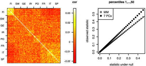
Figure 1: Left panel. An $80\times 80$ submatrix of the genetic correlation matrix of the non-UK individuals in the MS study. Ten randomly chosen individuals are shown for each of the following countries: FInland, SWeden, GErmany, IReland, POland, FRance, ITaly and SPain. The colors correspond to the pairwise correlation coefficients according to the scale in the middle. The diagonal values are close to 1.0 and are colored white. Right panel. The association test statistics of 470,000 SNPs plotted from the 1st percentile to the 50th (median). The null distribution on the $X$-axis is the chi-square with 1 df. Methods are the linear mixed model (MM) and the logistic regression with 7 leading principal components of the population structure as covariates (7PCs). The line is $y=x$.

We explored several approaches to address this issue. First we conducted a meta-analysis on groups that had balanced case–control ratios and were genetically homogeneous, according to a model-based clustering algorithm. We also conducted logistic regression by including the seven leading principal components (PCs) of the population structure as covariates [Patterson, Price and Reich (2006)]. A standard way of checking GWAS analysis is based on the assumption that only a very small proportion of the variants affect the phenotype and, therefore, the test statistics of the majority of the variants should follow the null distribution [Devlin, Roeder and Wasserman (2001)]. This assumption is often assessed through the “genomic control” parameter, $\lambda$, defined as the ratio of the median of the observed test statistic distribution to that of the theoretical null distribution. A substantial inflation was observed with $\lambda=1.44$ for the clustering approach and $\lambda=1.22$ for the PC approach (Figure 1). Although some of the inflation was likely to reflect the polygenic architecture of the disease (small genetic effects at very many variants) [Yang et al. (2011)], it remained likely that the underlying population structure was confounding the tests.

The linear mixed model as presented in this paper provided a way to include the whole estimated genetic correlation structure of 20,119 individuals in the regression model. The model-checking confirmed that the confounding effects were well controlled ($\lambda=1.02$, see Figure 1) while simultaneously the method maintained power to detect associations, as evidenced through the replication of over 20 previously-known associations. The main results of the MS GWAS, analyzed via the linear mixed model, included the identification of 29 novel association signals. These signals had important biological consequences, with further analyses showing that immunological genes are significantly overrepresented near the identified loci. In particular, the findings highlight an important role for T-helper-cell differentiation in the pathogenesis of MS. Another striking pattern was the very substantial overlap between genetic variants associated with MS and those associated with autoimmune diseases [see IMSGC and WTCCC2 (2011) for further details].

3 Binary data

The linear mixed model (1) is formulated for a univariate quantitative response and, therefore, its application to binary case–control data requires further justification. A connection between the standard linear model and the Armitage trend test [Armitage (1955)] that we derive in the supplementary text [Pirinen, Donnelly and Spencer (2013)] adds to the work of Astle and Balding (2009) and Kang et al. (2010) who have previously used the mixed model for significance testing in case–control GWAS. In addition to testing, it is also important to measure the effect sizes on a relevant scale. Next we explain how the output from the standard linear model can be turned into accurate effect size estimates on the log-odds scale, which is a natural scale for case–control studies.

For 0–1 valued responses $\mathbf{Y}=(y_{1},\ldots,y_{n})^{T}$ a logistic regression model assumes that

$$p_{i}=P(y_{i}=1|\mathbf{X},\bolds\gamma)=\frac{\exp(\mathbf{X}_{i}\bolds\gamma)}{1+\exp(\mathbf{X}_{i}\bolds\gamma)},$$ (4)

where the row $i$ of $\mathbf{X}$ is denoted by $\mathbf{X}_{i}$ and the effects of the predictors are in the vector $\bolds\gamma$. The score function of the corresponding binomial likelihood for a set of independent observations is $\mathbf{X}^{T}(\mathbf{Y}-\mathbf{p})$, where $\mathbf{p}=(p_{1},\ldots,p_{n})^{T}$ is a function of $\bolds\gamma.$ If we can justify a linear approximation $\mathbf{p}\approx\mathbf{X}\bolds\beta$, then the score becomes approximately zero at the least squares estimate $\widehat{\bolds\beta}=(\mathbf{X}^{T}\mathbf{X})^{-1}\mathbf{X}^{T}\mathbf{Y}$. In the supplementary text we argue that such an approximation is good when the logistic model effects $\bolds\gamma$ are small and we provide a connection between the parameters $\bolds\gamma$ and $\bolds\beta$ in those cases. These steps allow us to use the output from the standard linear model (i.e., the least squares solution $\widehat{\bolds\beta}$) to approximate the maximum likelihood estimates of the logistic regression model. For our GWAS application, where the case–control status is regressed on the population mean and the (mean-centered) reference allele count at a SNP, these considerations lead to the following estimate of the genetic effect on the log-odds scale:

$$\widehat{\beta}\biggl{(}\phi(1-\phi)+0.5(1-2\phi)(1-2\theta)\widehat{\beta}$$

(5)

$$\qquad{}-\frac{0.084+0.9\phi(1-2\phi)\theta(1-\theta)}{\phi(1-\phi)}\widehat{\beta}^{2}\biggr{)}^{-1},$$

where $\phi$ is the proportion of the cases in the data, $\theta$ is the reference allele frequency in the data and $\widehat{\beta}$ is the least squares estimate of the effect of the (mean-centered) reference allele count on the binary case–control status.

To investigate how well this approximation works in typical GWAS settings, we simulated case–control data for 5000 unrelated individuals at 500 SNPs for nine case proportions $\phi\in\{0.1,0.2,\ldots,0.9\}$. The allelic log-odds ratios $\gamma$ were taken from an equally spaced grid on the interval corresponding to odds ratios in $[1.0,1.3]$. This range covers typical GWAS hits; for example, in our MS study the median effect size among the 52 reported associations was 1.11 (minimum 1.08, maximum 1.22). In our MS study the lowest minor allele frequency among the variants taken to replication was 4.6%, which motivated us to sample the risk allele frequencies for the controls from a $\operatorname{Beta}(2,2)$ distribution, truncated to the interval $(0.05,\ldots,0.95)$. The frequencies in cases were determined by assuming that each copy of the risk allele increases log-odds of the disease additively by $\gamma$. Both linear and logistic regression models were then applied to the data with the population mean and the sampled genotypes as predictors. The differences in log-odds estimates $\widehat{\gamma}$ and their standard errors together with the $p$-values from the likelihood-ratio tests are shown in Figure 2, where the parameter estimates from the linear model have been transformed according to formula (3).

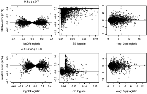
Figure 2: Difference between the linear and the logistic model. The panels include results from 2500 (top-row) and 2000 (bottom row) binary variants simulated as described in the text. The titles on the leftmost panels show the proportion of cases, $\phi$, $y$-axes show the relative differences between the linear and the logistic models in percentages and $x$-axes show the results from the logistic model. $\log\mathrm{OR}$, log-odds ratio; SE, standard error; $-\log 10(p)$, $-\log 10$ of the $p$-value from the likelihood-ratio test.

The conclusion from Figure 2 is that in a typical case–control GWAS data set where genetic effects are small, the case–control ratio is well-balanced and allele frequencies are not extreme (say, $\mathrm{OR}\leq 1.3$, $0.30\leq\phi\leq 0.70$ and $0.05<\mathrm{freq}<0.95$), the standard linear model provides an accurate approximation of the corresponding logistic regression model. The relative errors in the log-odds estimates or their standard errors are at most around 1% and in the $-\log 10$ $p$-values at most around 4% (top row of Figure 2). This result is useful because it suggests a natural way to apply the linear mixed model to binary data by using generalized least squares estimates (details in the supplementary text). The following empirical results show that this procedure performed well in our application.

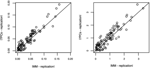
Figure 3: Absolute differences of 93 effect sizes between multiple sclerosis non-UK discovery and replication studies. Scales are log-odds (Left panel) and standardized log-odds (Right panel). MM: the linear mixed model in the discovery data; 7PCs: logistic regression with 7 principal components of genetic structure as covariates in the discovery data; replication: the replication data analyzed with logistic regression. Points above the diagonal: $62/93$ (Left) and $59/93$ (Right).

In our multiple sclerosis study we took 93 independent SNPs to the replication phase. The replication analysis was conducted with 4218 cases and 7296 controls using logistic regression [for details see IMSGC and WTCCC2 (2011)]. Figure 3 shows the absolute difference between the effect sizes in replication analysis and in the non-UK part of the discovery analysis using the linear mixed model ($x$-axes) and logistic regression including 7 principal components as covariates ($y$-axes). The log-odds ratios estimated by the linear mixed model were closer to the replication results in 62 out of 93 SNPs (one-sided binomial $p$-value 0.0009). The same pattern was present when the absolute differences are standardized (59 out of 93, $p=0.006$), suggesting that the methods presented here for estimating the log-odds ratios by the linear mixed model can lead to more accurate estimates than standard logistic regression analyses when the data contain complex correlation structure which, for practical reasons, cannot be fully included in a logistic regression model.

Obtaining effect size estimates and their standard errors is critical in the genetics context both in interpreting the results of individual studies and in combining results, via meta-analysis, across studies.

4 Maximum likelihood computation

The main analysis of our multiple sclerosis study was based on maximum likelihood (ML). In this section we consider how to efficiently maximize the likelihood function corresponding to the sampling distribution

$$\mathbf{Y}|\bigl{(}\bolds\beta,\sigma^{2},\eta\bigr{)}\sim\mathcal{N}\bigl{(}\mathbf{X}\bolds\beta,\eta\sigma^{2}\mathbf{R}+(1-\eta)\sigma^{2}\mathbf{I}\bigr{)},$$ (6)

with respect to $\bolds\beta,\eta$ and $\sigma^{2}$.

In general, finding the ML estimates for linear mixed models requires iterative procedures with expensive matrix operations [Lynch and Walsh (1998), page 787], but for the particular model (6) more efficient algorithms can be found. To our knowledge, the most efficient published algorithm is EMMA [Kang et al. (2008)], which has been applied to several recent GWAS [Atwell et al. (2010), Boyko et al. (2010)]. The algorithm FMM by Astle (2009), which is currently being implemented in the software suite GenABEL [Aulchenko et al. (2007)], was faster than EMMA in our test cases but, to date, its exact computational details have not been published. Another implementation of EMMA is in the software package TASSEL (currently v.3.0) [Bradbury et al. (2007)], which provides a graphical interface and several approximations to reduce the running time.

Next we describe a novel conditional maximization algorithm which is an order of magnitude faster than EMMA and was also faster than FMM in our tests except with the smallest sample size of $n=250$ individuals. We also consider in which situations the full ML estimation is more powerful than a recently proposed generalized least squares approximation [Kang et al. (2010), Zhang et al. (2010)], and compare the available methods. Finally, we give running times on our MS data set.

4.1 Conditional maximization

Our contribution to the ML estimation under the model (6) is a transformation of the data and predictors in such a way that the covariance matrix becomes diagonal, enabling an efficient conditional maximization procedure. This transformation is a direct extension of that used in general linear models to handle nondiagonal covariance matrices to a more general case of two variance components.

The eigenvalue decomposition of the positive semi-definite matrix $\mathbf{R}$ yields an orthonormal $n\times n$-matrix $\mathbf{U}$ of eigenvectors and a diagonal $n\times n$-matrix $\mathbf{D}$ of nonnegative eigenvalues for which $\mathbf{R}=\mathbf{U}\mathbf{D}\mathbf{U}^{T}$ [see Golub and Van Loan (1996)]. Let us write $\widetilde{\mathbf{Y}}=\mathbf{U}^{T}\mathbf{Y},\widetilde{\mathbf{X}}=\mathbf{U}^{T}\mathbf{X},$ and $\widetilde{\bolds\Sigma}=\eta\mathbf{D}+(1-\eta)\mathbf{I}.$ Then the log-likelihood function is

$$L\bigl{(}\bolds\beta,\eta,\sigma^{2}\bigr{)} = c-\frac{n}{2}\log\bigl{(}\sigma^{2}\bigr{)}-\frac{1}{2}\log\bigl{(}|\widetilde{\bolds\Sigma}|\bigr{)}$$

$${}-\frac{1}{2\sigma^{2}}(\widetilde{\mathbf{Y}}-\widetilde{\mathbf{X}}\bolds\beta)^{T}\widetilde{\bolds\Sigma}^{-1}(\widetilde{\mathbf{Y}}-\widetilde{\mathbf{X}}\bolds\beta),$$

where $c=-\frac{n}{2}\log(2\pi)$ and $|\widetilde{\bolds\Sigma}|$ denotes the determinant of $\widetilde{\bolds\Sigma}$ (details in the supplementary text).

Note that $\mathbf{U},\mathbf{D}$ and $\widetilde{\mathbf{Y}}$ are independent of $\mathbf{X}$ and that $\widetilde{\bolds\Sigma}$ is a diagonal matrix which allows efficient computation of the inverse and the determinant. After the eigenvalue decomposition of matrix $\mathbf{R}$ [complexity is $\mathcal{O}(n^{3})$], for each $\mathbf{X}$ the computation of $\widetilde{\mathbf{X}}$ requires $\mathcal{O}(kn^{2})$ operations where $k\leq K$ is the number of columns of $\mathbf{X}$ that need to be recomputed, and for each set of values of the parameters the evaluation of the log-likelihood requires $\mathcal{O}(nK)$ operations. To maximize the log-likelihood, we apply a standard optimization technique of conditional maximization as described in the supplementary text.

4.2 GLS approximation

In settings where the variance parameter $\eta$ does not vary much between the analyzed $\mathbf{X}$ matrices, an efficient approximation can be found by estimating $\eta$ only once and then applying a generalized least squares (GLS) method to approximate the ML estimates of $\bolds\beta$ and $\sigma^{2}$ for any given $\mathbf{X}$ matrix while $\eta$ is kept fixed. This idea has been implemented in the software packages EMMAX [Kang et al. (2010)] and TASSEL [Zhang et al. (2010)]; similar ideas had been proposed earlier by Aulchenko, de Koning and Haley (2007). We will call this approach the GLS approximation to the full model.

The GLS approximation is accurate only if $\eta$ does not vary much between different sets of predictors, for example, when the individual predictors explain only a negligible proportion of the total variance of the response. This situation is typical in current GWAS studies on humans, as the still unidentified genetic effects are small. For example, in our MS study there were no noticeable differences between the full likelihood analysis and the GLS approximation, and in their simulation study Zhang et al. (2010) did not find significant differences in the statistical power between the two methods. However, if the data contain closely related individuals and individual genetic effects explain enough phenotypic variation, then the full likelihood analysis may have higher power than the GLS approximation, as we demonstrate below. With our efficient implementation of the full model it is possible to study this in more detail than before.

Family example

We consider children of 25 independent families, each with 6 full-siblings and a quantitative phenotype of whose variance 15% is explained by a major gene and 8.5% by minor genes (heritability is 23.5%). The remaining 76.5% of the variation in the phenotype is independent of the family structure.

We simulated 10 million such phenotypes and paired each with a set of simulated genotypes that were independent of the phenotype (given the family structure). The minor allele frequency was chosen uniformly between 0.25 and 0.5, and Hardy–Weinberg equilibrium [see, e.g., Lynch and Walsh (1998)] was assumed. We used these data sets to get accurate estimates of the threshold values of the likelihood ratio statistic under the null hypothesis of no genetic effect down to type I error $10^{-4}$.

We then simulated an additional one million phenotypes, but this time tested the genotypes of the major gene that influenced each phenotype. Using the empirical threshold values (with their 95% confidence intervals) from the null simulations, the top two rows of Table 2 show the power of the linear mixed model (MM), the GLS approximation and the standard linear model (LM) at type I errors $10^{-3}$ and $10^{-4}$. In both cases MM is more powerful than the GLS approximation, which in turn is more powerful than LM.

Table 2: Power in family data. Columns: $\alpha$, type I error rate; MM, linear mixed model; GLS, generalized least squares approximation; LM, standard linear model. Cells give estimates of power together with their 95% confidence intervals. The first two rows are based on the empirical type I error thresholds and the remaining four rows use theoretical thresholds

$\bolds{\alpha}$	MM	GLS	LM
Empirical
$10^{-3}$	0.914	0.910	0.890
	(0.913..0.915)	(0.909..0.911)	(0.889..0.891)
$10^{-4}$	0.762	0.751	0.708
	(0.757..0.767)	(0.746..0.757)	(0.702..0.714)
Theoretical
$10^{-3}$	0.914	0.903	0.887
	(0.913..0.914)	(0.903..0.904)	(0.886..0.887)
$10^{-4}$	0.760	0.732	0.702
	(0.759..0.761)	(0.731..0.733)	(0.701..0.703)
$10^{-6}$	0.338	0.293	0.265
	(0.337..0.339)	(0.292..0.294)	(0.264..0.266)
$5\times 10^{-8}$	0.145	0.115	0.099
	(0.144..0.145)	(0.114..0.115)	(0.098..0.099)

Table 3: Ratios of observed quantiles to expected. Columns: $\alpha$, upper quantile; EXPECTED, theoretical 95% confidence interval for the ratio in $10^{7}$ samples; MM, linear mixed model; GLS, generalized least squares approximation; LM, standard linear model. Values outside the interval are in bold

$\bolds{\alpha}$	EXPECTED	MM	GLS	LM
$10^{-3}$	0.997..1.003	0.998	0.979	0.990
$10^{-4}$	0.992..1.008	0.997	0.973	0.992
$10^{-5}$	0.981..1.019	1.001	0.969	1.002

In practice, inferences in GWAS are based on the asymptotic large-sample properties of the test statistics. As mentioned in Section 2, a widely-used method for checking how well the asymptotics hold is to assess the ratio of the medians of the observed and expected (chi-square) test statistic distributions, denoted by $\lambda$ [Devlin, Roeder and Wasserman (2001)]. For a sample of $10^{7}$ draws from the theoretical null distribution the (analytically calculated) upper bound of the 95% confidence interval of $\lambda$ is 1.0014, whereas in our $10^{7}$ null simulations we observed values 1.055, 1.031 and 1.280 for MM, GLS approximation and LM, respectively. Even though accounting for families has brought MM and GLS much closer to the asymptotic null distribution compared to LM, both methods are still inflated with respect to the theoretical distribution in this example with a fairly small sample size. Note that the GLS approximation always results in smaller likelihood ratio statistics, and thus smaller $\lambda$ values, than MM since GLS does not maximize the full model under the alternative whereas MM does.

A simple way to make the observed test statistics match better with the theoretical distribution is to divide them by their corresponding estimates of $\lambda$, a procedure called genomic control (GC) [Devlin, Roeder and Wasserman (2001)]. In this example GC works well but since it treats all the variants the same, it is not an ideal method for controlling for confounding in more complex scenarios where different loci have very different population genetic histories [Astle and Balding (2009)]. Therefore, we have not used it with the MS data set.

Table 3 shows the ratios of some quantiles of the observed distributions to their theoretical values after genomic control, together with the theoretical 95% intervals of those ratios assuming $10^{7}$ draws from the null distribution. We observe no deviation from the theoretical distribution for the linear mixed model and only a slight deflation for the standard linear model, but the GLS approximation is deflated throughout the range of quantiles considered. Whether this phenomenon is specific to the family data considered or holds more generally requires further investigation. The lower panel of Table 2 shows power at the theoretical thresholds corresponding to type I error rates relevant in GWAS, after genomic control was applied to the one million nonnull tests. The relative power difference between MM and the GLS approximation increases with decreasing type I errors.

In this example MM was noticeably more powerful than the GLS approximation, both at the empirical and theoretical thresholds, after making the inflated statistics comparable by genomic control. On the other hand, if neither empirical thresholds nor genomic control parameters were available, then the GLS approximation could be a more robust choice in small data sets as reflected by the observed $\lambda$ values in this example.

4.3 Comparing methods

Our conditional maximization (CM) algorithm, EMMA and the GLS approximation all make use of a decomposition of the $\mathbf{R}$ matrix requiring $\mathcal{O}(n^{3})$ operations: [(iii)]

EMMA requires an additional $\mathcal{O}(n^{3})$ matrix decomposition for each set of predictors $\mathbf{X}$, whereas CM and GLS are $\mathcal{O}(n^{2})$ algorithms for each $\mathbf{X}$ given the initial decomposition of $\mathbf{R}$.

EMMA reduces the problem to one-dimensional optimization for which the global maximum is in theory more reliably found than by using CM.

Parameterization of the model through $\eta$ (CM) has a computational advantage over parameterization using $\delta=(1-\eta)/\eta$ (EMMA) since the maximization is easier over the compact set $\eta\in[0,1]$ than over the unbounded interval $\delta\in[0,\infty)$.

It is expected that the GLS approximation is computationally more efficient but in some cases less accurate in ML estimation, and less powerful in testing the predictors than either EMMA or CM, as demonstrated with the previous family example.

We investigated through simulation studies how the above differences manifest themselves in practice, related to the reliability and running time of the algorithms. We applied the EMMA R-package v.1.1.2 [Kang et al. (2008)] with the default parameters and our C-implementation of the CM algorithm (software package MMM). For the time comparisons we also included a GLS approximation (our C-implementation in software package MMM) and a beta version of the algorithm FMM [Astle (2009)]. We note that the software package TASSEL relies on the EMMA algorithm in full ML estimation, and for the GLS approximation both TASSEL and EMMAX are similar to our GLS implementation. Therefore, TASSEL and EMMAX were not included in these comparisons.

4.3.1 Reliability

The purpose of these tests is to assess whether condition (ii) above has any practical effect on the variance parameter estimation. For each value of $\eta\in\{0,0.05,0.1,\ldots,0.95,1\}$ we generated 1000 data sets for $n=500$ subjects. A single data set consisted of an $\mathbf{R}$ matrix and a $\mathbf{Y}$ vector. To create $\mathbf{R}$, we simulated nonzero elements of an $n\times n$ lower triangular matrix $\mathbf{L}$ from the standard normal distribution and set $\mathbf{R}=\mathbf{L}\mathbf{L}^{T}$ with the extra condition that if some of the eigenvalues of $\mathbf{L}\mathbf{L}^{T}$ were $<10^{-3}$ they were set to $10^{-3}$ to guarantee that $\mathbf{R}$ was numerically positive-definite. (The largest condition number of $\mathbf{R}$ matrices was $1.5\times 10^{6}$.) $\mathbf{Y}$ was then simulated according to the model $\mathbf{Y}=\bolds\varrho+\bolds\varepsilon$, where $\bolds\varrho\sim\mathcal{N}(0,\eta\mathbf{R})$ and $\bolds\varepsilon\sim\mathcal{N}(0,(1-\eta)\mathbf{I})$. The ML estimates of $\eta$ and $\sigma^{2}$ were obtained from EMMA and the CM algorithm. Since FMM does not output the value of the maximized log-likelihood, we have not included it in this comparison. Also, for these data sets, the GLS approximation is the same as the full model since we use each $\mathbf{R}$ matrix only once. Thus, no separate results for GLS are reported.

Table 4: Maximum absolute differences between EMMA and CM and the ranges of the estimated quantities over 19,000 simulated data sets with $0.05\leq\eta\leq 0.95$

	max log-likelihood	$\bolds{\sigma^{2}}$	$\bolds{\eta}$
$\max\Delta$	0.0053	$3.0\cdot 10^{-5}$	$1.2\cdot 10^{-5}$
Range	($-1618.332$, $-1085.829$)	(0.601, 1.444)	(0.029, 0.976)

The results for 19,000 data sets simulated with $0.05\leq\eta\leq 0.95$ were the same between the methods for all practical purposes (Table 4). In addition to being similar up to 3 decimal places, the optimized log-likelihood values had no tendency of being higher with one algorithm than with the other ($p=0.46$ in the two-sided binomial test).

When $\eta$ was on the boundary $\{0,1\}$ the CM algorithm found points where the log-likelihood was at least 0.01 higher than that found by EMMA in 1503 cases out of the 2000 data sets (maximum of these differences was 1.06). This is due to property (iii) above, which requires EMMA to constrain the search to a compact subset of its unbounded search space. The size of the search space is a parameter of EMMA [we used the default values of $-10<\log(\delta)<10$] and by increasing this interval higher likelihood values could be found also by EMMA, but with higher computational cost. Alternatively, one could parameterize EMMA using $\eta$ instead of $\delta$, in which case EMMA and CM would be expected to give the same results also on the boundary $\eta\in\{0,1\}$.

Thus, even if in theory the CM algorithm does not have guaranteed convergence to the global optimum, in practice, it has found the same maxima as EMMA in all 19,000 cases with $\eta\in\{0.05,\ldots,0.95\}$. Furthermore, in the great majority of the remaining boundary cases $\eta\in\{0,1\}$ the CM algorithm has actually found a point with a higher likelihood value than EMMA. Since we generated the covariance matrices randomly without any particular structure, these results suggest that the CM algorithm is a reliable method for the general problem of ML estimation in the linear mixed model that we consider.

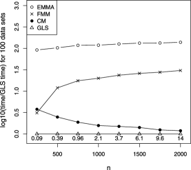
Figure 4: Relative running times for 100 data sets compared to GLS, on the $\log 10$ scale, as a function of the sample size $n$. Methods are the R-package EMMA v.1.1.2, our C-implementations of conditional maximization (CM) and generalized least squares (GLS) and a C-implementation of FMM (downloaded in March 2011). The figures below the GLS-line are the GLS times in seconds. Note that GLS is less accurate than the other three methods which have fairly similar accuracy to each other.

4.3.2 Running time

In applications, such as genome-wide association studies, where a single covariance matrix $\mathbf{R}$ is repetitively used with several sets of predictors $\mathbf{X}$, there is a large difference in the running times between CM and EMMA due to property (i) above. To investigate this difference, for each $n\in\{250,500,\ldots,2000\}$, we simulated a single $\mathbf{R}$ matrix and $\mathbf{Y}$ vector as above, together with 100 different $\mathbf{X}$ matrices. Each $\mathbf{X}$ had dimension $n\times 2$ and the first column was always vector $\mathbf{1}$ to model the population mean and the second column contained a randomly sampled binary vector where each element was 1 with probability 0.5 and 0 otherwise. The likelihood ratio (LR) tests for the effects $\beta_{2}$ were carried out using EMMA, FMM and our implementations of the CM and GLS algorithms.

Figure 4 presents the running times as compared to the GLS approximation. We see that independently of the sample size, EMMA takes about 100 times the time of the GLS procedure, reflecting the fact that EMMA carries out an additional $n\times n$-matrix decomposition for each of the 100 data sets.

The relative efficiency of the GLS procedure over CM decreases as the sample size grows, because both methods initialize the data similarly by computing $\widetilde{\mathbf{X}}=\mathbf{U}^{T}\mathbf{X}$, and this task takes a larger and larger proportion of the whole running time as $n$ grows. A similar trend of decreasing relative difference is also present when the initial matrix decomposition is subtracted from the running times of CM and GLS (results not shown).

The FMM algorithm is clearly faster than EMMA but slower than CM except for the smallest sample size $n=250$. We are not able to comment on the putative sources of these differences since the methodological details of FMM have not been published.

Table 5 shows the maximum differences between the methods in the likelihood ratio statistics and the estimates of $\eta$. We see that the results from EMMA and CM were again practically the same over all 800 data sets and even though FMM deviated slightly from the common results of EMMA and CM, it was clearly closer to those two methods than to GLS.

Table 5: Maximum absolute pairwise differences between EMMA, CM, FMM and GLS in likelihood ratio statistic (upper diagonal) and $\eta$ estimate (lower diagonal) over the 800 data sets of Figure 4

	EMMA	CM	FMM	GLS
EMMA	–	3.2$\times 10^{-4}$	0.089	0.43
CM	8.1$\times 10^{-6}$	–	0.089	0.43
FMM	0.004500.	0.0046000	–	0.34
GLS	0.029000.	0.0290000	0.027	–

Given these results, it seems that CM is a natural choice for likelihood inference in the linear mixed model (6) since it is much faster than EMMA, more accurate than GLS and still computationally feasible whenever GLS is.

4.4 MS data set

We applied the CM algorithm to the non-UK component of our multiple sclerosis GWAS data set (20,119 individuals and 520,000 SNPs). After the initial matrix decomposition was completed (in 3 hours 35 minutes), the running time was 19 minutes 10 seconds per 1000 SNPs using a single processor (Intel Xeon 2.50 GHz) and about 3GB of RAM, so the whole MS data set can be run in 7 days and 2 hours by using the CM algorithm on a single processor. If instead one were to apply a method such as EMMA, which requires a separate matrix decomposition at each SNP, we estimate that the corresponding running time of the whole MS data set would be about 210 years. As noted earlier, in GWAS where genetic effects are small, the GLS approximation (including programs EMMAX and TASSEL) is expected to give, in practice, the same results as the full likelihood analysis, and thus could also have been a possible choice for this data set. The running time of the GLS approximation on the MS data set is about 5 days 19 hours, that is, 18% less than that of CM.

5 Bayes factors

A Bayesian framework provides a fully probabilistic quantification of the association evidence, which is a useful complement to the traditional frequentist interpretation in the GWAS context [Wakefield (2009)]. It also allows use of prior knowledge, for example, a particular dependency between the allele frequency and the effect size. This possibility becomes more and more important as our understanding about the genetic architecture of complex traits develops [Stephens and Balding (2009)].

In a Bayesian version of the linear mixed model (1), in addition to the priors (2) for the random effects, we adopt the following priors:

$$\bigl{(}\bolds\beta,\sigma^{2}\bigr{)} \sim \mathrm{Normal\mbox{-}Inverse\mbox{-}Gamma}(\mathbf{m},\mathbf{V},a,b),$$

$$\eta \sim \operatorname{Beta}(r,t).$$

Here $a,b,r,t>0$ are scalar parameters, $\mathbf{m}$ is a $K$-dimensional vector and $\mathbf{V}$ is a $K\times K$ matrix. In the supplementary text we describe the properties of these priors and show how to efficiently evaluate the marginal likelihood of the data. The marginal likelihoods allow comparisons between models that differ in the structure of the predictor matrix $\mathbf{X}$ (e.g., testing genetic effects in GWAS), in the prior distributions of the parameters (e.g., whether $\eta=0$) or both.

5.1 Bayes factors for genetic association

In the non-UK component of our MS data set (20,119 individuals, 520,000 SNPs) the extra time spent in computing the Bayes factors for SNP effects compared to computing only the ML estimates was 2 minutes 13 seconds per 1000 SNPs (Intel Xeon 2.50 GHz), that is, an increase of about 12% in the running time. Following previous work [WTCCC (2007)], we chose the prior distribution on the genetic effect to be centered at $0$ and have standard deviation of 0.2 on the log-odds scale, independently of the allele frequency. With this choice there was nearly a linear relationship between the logarithmic $p$-values and the logarithmic Bayes factors (Figure 5). This data set-specific relationship provides useful information about these two conceptually different quantities.

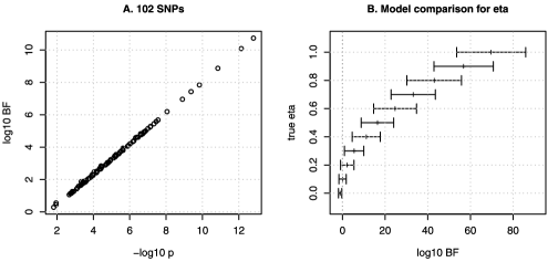
Figure 5: (A) Comparing $-\log 10$ $p$-values and $\log 10$ Bayes factors in the non-UK component of our MS study for 102 SNPs taken to replication. (B) Distribution of $\log 10$ Bayes factors between models $\eta\sim\operatorname{Uniform}(0,1)$ and $\eta=0$. For each value of $\eta\in\{0,0.1,\ldots,1\}$, 100 data vectors $\mathbf{Y}$ were simulated and means $\pm 2\times$standard deviations of the corresponding $\log 10\mathrm{BF}$ distributions are shown. The proportions of the data sets for which $\log 10(\mathrm{BF})>0$ were 0.01, 0.45 and 0.98, for true value of $\eta$ being 0.0, 0.1 and 0.2, respectively, and 1 whenever $\eta\geq 0.3$.

5.2 Estimating heritability from a population sample

Recently, Yang et al. (2010) estimated the proportion of the variance in human height that can be explained by a dense genome-wide collection of SNPs from a large sample of distantly related individuals. Here we demonstrate Bayesian computation by answering a related question of how high heritability (i.e., $\eta$ in our mixed model) needs to be in order to be detectably nonzero from a particular sample of distantly related individuals. Note, however, that we do not interpret $\eta$ as heritability in our MS data set due to the confounding effects of the population structure.

We consider a sample of $n=5340$ UK individuals including 2665 healthy blood donors recruited from the United Kingdom Blood Service (UKBS) and 2675 samples from the 1958 Birth Cohort (1958BC). These samples have been used as common controls for several GWAS carried out by the Wellcome Trust Case-Control Consortium 2. Here we focus on the genotype data generated by the Affymetrix 6.0 chip. After a quality control process, we made use of a genome-wide set of $S=168\mbox{,}351$ approximately independent SNPs to compute a pairwise genetic correlation matrix $\mathbf{R}=(r_{ij})$ for these individuals by setting

$$r_{ij}=\frac{1}{S}\sum_{s=1}^{S}\frac{(a_{s}^{(i)}-2p_{s})(a_{s}^{(j)}-2p_{s})}{2p_{s}(1-p_{s})},$$ (8)

where $a_{s}^{(i)}$ is the number of copies of allele 1 that individual $i$ carries at SNP $s$, $a_{s}^{(j)}$ is similarly defined for individual $j$, and $p_{s}$ is the frequency of allele 1 at SNP $s$ in the whole sample of $n$ individuals. The interpretation of $r_{ij}$ is that of relative genome-wide sharing of alleles compared to an average pair of individuals in the sample. In particular, negative (positive) $r_{ij}$ denotes more distant (closer) relatedness than that of an average pair in the sample, for whom the correlation is $r_{ij}=0$. The same matrix (divided by 2) is called a “kinship matrix” by Astle and Balding (2009) and, excepting a slight adjustment on the diagonal, it is also the same as the “raw” relatedness matrix used by Yang et al. (2010). For other versions of genetic relationship matrices, see, for example, Kang et al. (2008), Astle and Balding (2009). In our data all nondiagonal elements of $\mathbf{R}$ were below 0.03, showing that there were no close relatives within this sample.

We simulated 100 phenotype vectors $\mathbf{Y}$ for the individuals for each value of $\eta\in\{0,0.1,\ldots,1\}$ from the distribution $\mathbf{Y}\sim\mathcal{N}(0,\eta\mathbf{R}+(1-\eta)\mathbf{I})$. We then compared two versions, $M_{0}$ and $M_{1}$, of the linear mixed model

$$\mathbf{Y}=\beta+\bolds\varrho+\bolds\varepsilon\qquad\mbox{with }\bolds\varrho\sim\mathcal{N}(0,\eta\sigma^{2}\mathbf{R})\mbox{ and }\bolds\varepsilon\sim\mathcal{N}\bigl{(}0,(1-\eta)\sigma^{2}\mathbf{I}\bigr{)},$$

where in both models the prior on $(\beta,\sigma^{2})$ was $\operatorname{NIG}(m=0,V=10,a=10,d=12)$ and in $M_{0}\dvtx\eta=0$ and in $M_{1}\dvtx\eta\sim\operatorname{Uniform}(0,1)$. For each data set we computed marginal likelihoods $p(\mathbf{Y}|M_{1})$ and $p(\mathbf{Y}|M_{0})$ whose ratio gives the Bayes factor (BF), which tells how the prior odds of the models are updated to the posterior odds by the observed data $\mathbf{Y}$ [Kass and Raftery (1995)]. In particular, if BF${}>{}$1 [i.e., log10(BF)${}>{}$0], then the data favors model $M_{1}$ over model $M_{0}$, and if BF${}<{}$1 [i.e., log10(BF)${}<{}$0], then the opposite is true. Figure 5 shows the distributions of log10(BF) for different (true) values of $\eta$. The running time of computing BFs for all 1100 data sets was less than 5 minutes (Intel Xeon 2.50 GHz) after $\mathbf{R}$ had been decomposed once, which took another 4 minutes.

We conclude that in our data set the model $M_{0}$ is (correctly) favored in almost all the cases that were simulated with $\eta=0$ and that when the true $\eta\geq 0.3$, then it is very likely that model $M_{1}$ will be favored; that is, in these individuals we expect that this model comparison procedure detects nonzero heritability for the phenotypes that truly have heritabilities $\eta\geq 0.3.$ However, with real data there is a complication that the estimated $\mathbf{R}$ matrix does not completely capture the true genome-wide correlation, as only a subset of the relevant variation is used in estimating $\mathbf{R}$ [Yang et al. (2010)]. As a consequence, with real phenotype data the lower limit of a convincingly detectable $\eta$ is likely to be higher than in these simulations which have assumed that $\mathbf{R}$ is known exactly.

In general, the distribution of BFs depends on the sample size $n$, the relatedness structure $\mathbf{R}$ and the priors on $\eta$, and the formulae we have derived in the supplementary text provide a computationally efficient way to assess these dependencies in any particular data set.

6 Discussion

Motivated by genome-wide association studies (GWAS), we have presented computationally efficient ways to analyze the linear mixed model

$$\mathbf{Y}=\mathbf{X}\bolds\beta+\bolds\varrho+\bolds\varepsilon\qquad$$

$$\eqntext{\mbox{with }\bolds\varrho|\bigl{(}\eta,\sigma^{2}\bigr{)}\sim\mathcal{N}\bigl{(}0,\eta\sigma^{2}\mathbf{R}\bigr{)}\mbox{ and }\bolds\varepsilon|\bigl{(}\eta,\sigma^{2}\bigr{)}\sim\mathcal{N}\bigl{(}0,(1-\eta)\sigma^{2}\mathbf{I}\bigr{)}}$$ (9)

in situations where many $\mathbf{X}$ matrices are analyzed with a single covariance matrix $\mathbf{R}$. In the GWAS context the role of the random effect $\bolds\varrho$ is to control for those associations between phenotypes and genetic variants that can already be explained by the genome-wide genetic sharing. The mixed model approach is especially useful when the study individuals show a complex relatedness structure which cannot be captured by including a few linear predictors in the model. Such a situation may arise if a case–control study combines individuals from several populations with differing case–control ratios [e.g., IMSGC and WTCCC2 (2011)] or if the sampled individuals contain close relatives, for example, in studies of model organisms [Yu et al. (2005), Kang et al. (2008), Atwell et al. (2010)], domesticated animals [Boyko et al. (2010)] or humans with recent pedigree information [Aulchenko, de Koning and Haley (2007)].

For our case–control GWAS application [IMSGC and WTCCC2 (2011)] we have derived an accurate transformation between the linear and logistic regression models when the predictors have only small effects on the response. This approach has the great benefit of enabling interpretation of the linear mixed model results on the log-odds scale, which is important in the GWAS context both for understanding the sizes of the genetic effects and for combining the results via meta-analyses across independent studies.

We have also formulated a conditional maximization (CM) algorithm for maximum likelihood estimation which is an order of magnitude faster than the existing EMMA algorithm [Kang et al. (2008)] and in our tests was also faster than the FMM algorithm [Astle (2009)], except with the smallest sample size ($n=250$). With the small effect sizes that are typical in current GWAS the full mixed model analysis (performed by CM, EMMA and FMM) gives very similar results to the generalized least squares approximation (GLS) that has been implemented in EMMAX [Kang et al. (2010)] and TASSEL [Zhang et al. (2010)]. However, in other genetics contexts the full mixed model may be more powerful than the GLS approximation, as we demonstrated with an example that contained close relatives and genetic variants with large effects. Given that our CM approach is computationally only slightly more demanding than the GLS approximation (by about 20% in running time in our large MS data set), it seems well-suited for routine use in genetics applications.

We also considered computation of Bayes factors for the genetic associations as well as for the variance components. Another possible application of the Bayesian model is in predicting an unobserved response $y_{i}$ based on the set of observed values $\mathbf{Y}_{-i}=(y_{1},\ldots,y_{i-1},y_{i+1},\ldots,y_{n})^{T}$ and the model $M$ (which contains information on priors, $\mathbf{X}$ and $\mathbf{R}$). The required posterior $p(y_{i}|\mathbf{Y}_{-i},M)\propto p(y_{i},\mathbf{Y}_{-i}|M)$ can be efficiently calculated on a grid of possible values $y_{i}$ by using the methods described in the supplementary text. These calculations are especially simple if response $y_{i}$ is restricted to a set of discrete values as is the case with binary data.

A natural question is whether the efficient computational solutions presented in this article could be extended to linear mixed models with more random effects, as, for example, when analyzing gene expression data with both the genetic relatedness and the expression heterogeneity as random effects [Listgarten et al. (2010)]. The key issue that made the CM algorithm fast in our application was the ability to diagonalize the full covariance matrix $\bolds\Sigma$ by using an orthonormal matrix $\mathbf{U}$ which did not depend on the variance parameters, or, in other words, $\mathbf{R}$ and $\mathbf{I}$ were simultaneously diagonalizable by the same orthonormal $\mathbf{U}$. More generally, a set of symmetric matrices is simultaneously diagonalizable by an orthonormal matrix if and only if the matrices commute [Schott (2005), Theorem 4.18]. Thus, the computational strategy that we used here generalizes straightforwardly only to a rather special case of commutable covariance matrices. In other situations an approximation to the full model could be achieved by the generalized least squares approximation where the variance parameters are estimated only once and then kept fixed for the repeated analysis of different predictor sets [Kang et al. (2010), Zhang et al. (2010)]. On the other hand, an efficient generalization of both CM and EMMA to multiple response vectors $\mathbf{Y}$ is straightforward since the necessary matrix decompositions do not depend on $\mathbf{Y}$. This feature was utilized in our example of heritability estimation.

Extending linear mixed models to proper variable selection models that simultaneously analyze several thousands of predictors is also an important topic. Further work is required to determine whether the computational solutions presented in this work can help implement more complex variable selection models.

Even though GWAS and other genetics applications have given the main motivation for this study, our results are more generally valid for any application that fits into the framework of the standard linear model with one additional normally distributed random effect.

References

- Armitage (1955) {barticle}[author] \bauthor\bsnmArmitage, \bfnmP.\binitsP. (\byear1955). \btitleTests for linear trends in proportions and frequencies. \bjournalBiometrics \bvolume11 \bpages375–386. \bptokimsref \endbibitem
- Astle (2009) {bmisc}[author] \bauthor\bsnmAstle, \bfnmW.\binitsW. (\byear2009). \bhowpublishedPopulation structure and cryptic relatedness in genetic association studies. Ph.D. thesis, Univ. London. \bptokimsref \endbibitem
- Astle and Balding (2009) {barticle}[mr] \bauthor\bsnmAstle, \bfnmWilliam\binitsW. and \bauthor\bsnmBalding, \bfnmDavid J.\binitsD. J. (\byear2009). \btitlePopulation structure and cryptic relatedness in genetic association studies. \bjournalStatist. Sci. \bvolume24 \bpages451–471. \biddoi=10.1214/09-STS307, issn=0883-4237, mr=2779337 \bptokimsref \endbibitem
- Atwell et al. (2010) {barticle}[author] \bauthor\bsnmAtwell, \bfnmS.\binitsS., \bauthor\bsnmHuang, \bfnmY. S.\binitsY. S., \bauthor\bsnmVilhjalmsson, \bfnmB. J.\binitsB. J., \bauthor\bsnmWillems, \bfnmG.\binitsG., \bauthor\bsnmHorton, \bfnmM.\binitsM., \bauthor\bsnmLi, \bfnmY.\binitsY. \betalet al. (\byear2010). \btitleGenome-wide association study of 107 phenotypes in Arabidopsis thaliana inbred lines. \bjournalNature \bvolume465 \bpages627–631. \bptokimsref \endbibitem
- Aulchenko, de Koning and Haley (2007) {barticle}[pbm] \bauthor\bsnmAulchenko, \bfnmYurii S.\binitsY. S., \bauthor\bparticlede \bsnmKoning, \bfnmDirk-Jan\binitsD.-J. and \bauthor\bsnmHaley, \bfnmChris\binitsC. (\byear2007). \btitleGenomewide rapid association using mixed model and regression: A fast and simple method for genomewide pedigree-based quantitative trait loci association analysis. \bjournalGenetics \bvolume177 \bpages577–585. \biddoi=10.1534/genetics.107.075614, issn=0016-6731, pii=genetics.107.075614, pmcid=2013682, pmid=17660554 \bptokimsref \endbibitem
- Aulchenko et al. (2007) {barticle}[author] \bauthor\bsnmAulchenko, \bfnmY. S.\binitsY. S., \bauthor\bsnmRipke, \bfnmS.\binitsS., \bauthor\bsnmIsaacs, \bfnmA.\binitsA. and \bauthor\bparticlevan \bsnmDuijn, \bfnmC. M.\binitsC. M. (\byear2007). \btitleGenABEL: An R library for genome-wide association analysis. \bjournalBioinformatics \bvolume23 \bpages1294–1296. \bptokimsref \endbibitem
- Boyko et al. (2010) {barticle}[pbm] \bauthor\bsnmBoyko, \bfnmAdam R.\binitsA. R., \bauthor\bsnmQuignon, \bfnmPascale\binitsP., \bauthor\bsnmLi, \bfnmLin\binitsL. and \bauthor\bsnmSchoenebeck, \bfnmJeffrey J.\binitsJ. J. \betalet al. (\byear2010). \btitleA simple genetic architecture underlies morphological variation in dogs. \bjournalPLoS Biol. \bvolume8 \bpagese1000451. \biddoi=10.1371/journal.pbio.1000451, issn=1545-7885, pmcid=2919785, pmid=20711490 \bptokimsref \endbibitem
- Bradbury et al. (2007) {barticle}[pbm] \bauthor\bsnmBradbury, \bfnmPeter J.\binitsP. J., \bauthor\bsnmZhang, \bfnmZhiwu\binitsZ., \bauthor\bsnmKroon, \bfnmDallas E.\binitsD. E., \bauthor\bsnmCasstevens, \bfnmTerry M.\binitsT. M., \bauthor\bsnmRamdoss, \bfnmYogesh\binitsY. and \bauthor\bsnmBuckler, \bfnmEdward S.\binitsE. S. (\byear2007). \btitleTASSEL: Software for association mapping of complex traits in diverse samples. \bjournalBioinformatics \bvolume23 \bpages2633–2635. \biddoi=10.1093/bioinformatics/btm308, issn=1367-4811, pii=btm308, pmid=17586829 \bptokimsref \endbibitem
- Devlin, Roeder and Wasserman (2001) {barticle}[author] \bauthor\bsnmDevlin, \bfnmB.\binitsB., \bauthor\bsnmRoeder, \bfnmK.\binitsK. and \bauthor\bsnmWasserman, \bfnmL.\binitsL. (\byear2001). \btitleGenomic control, a new approach to genetic-based association studies. \bjournalTheor. Pop. Biol. \bvolume60 \bpages155–166. \bptokimsref \endbibitem
- Fisher (1918) {barticle}[author] \bauthor\bsnmFisher, \bfnmR. A.\binitsR. A. (\byear1918). \btitleThe correlation between relatives on the supposition of Mendelian inheritance. \bjournalTransactions on Royal Society of Edinburgh \bvolume52 \bpages399–433. \bptokimsref \endbibitem
- Golub and Van Loan (1996) {bbook}[mr] \bauthor\bsnmGolub, \bfnmGene H.\binitsG. H. and \bauthor\bsnmVan Loan, \bfnmCharles F.\binitsC. F. (\byear1996). \btitleMatrix Computations, \bedition3rd ed. \bpublisherJohns Hopkins Univ. Press, \blocationBaltimore, MD. \bidmr=1417720 \bptokimsref \endbibitem
- IMSGC and WTCCC2 (2011) {bmisc}[author] \borganizationIMSGC and \borganizationWTCCC2 (\byear2011). \bhowpublishedGenetic risk and a primary role for cell-mediated immune mechanisms in multiple sclerosis. Nature 476 214–219. \bptokimsref \endbibitem
- Kang et al. (2008) {barticle}[pbm] \bauthor\bsnmKang, \bfnmHyun Min\binitsH. M., \bauthor\bsnmZaitlen, \bfnmNoah A.\binitsN. A., \bauthor\bsnmWade, \bfnmClaire M.\binitsC. M., \bauthor\bsnmKirby, \bfnmAndrew\binitsA., \bauthor\bsnmHeckerman, \bfnmDavid\binitsD., \bauthor\bsnmDaly, \bfnmMark J.\binitsM. J. and \bauthor\bsnmEskin, \bfnmEleazar\binitsE. (\byear2008). \btitleEfficient control of population structure in model organism association mapping. \bjournalGenetics \bvolume178 \bpages1709–1723. \biddoi=10.1534/genetics.107.080101, issn=0016-6731, pii=178/3/1709, pmcid=2278096, pmid=18385116 \bptokimsref \endbibitem
- Kang et al. (2010) {barticle}[pbm] \bauthor\bsnmKang, \bfnmHyun Min\binitsH. M., \bauthor\bsnmSul, \bfnmJae Hoon\binitsJ. H., \bauthor\bsnmService, \bfnmSusan K.\binitsS. K., \bauthor\bsnmZaitlen, \bfnmNoah A.\binitsN. A., \bauthor\bsnmKong, \bfnmSit-Yee\binitsS.-Y., \bauthor\bsnmFreimer, \bfnmNelson B.\binitsN. B., \bauthor\bsnmSabatti, \bfnmChiara\binitsC. and \bauthor\bsnmEskin, \bfnmEleazar\binitsE. (\byear2010). \btitleVariance component model to account for sample structure in genome-wide association studies. \bjournalNat. Genet. \bvolume42 \bpages348–354. \biddoi=10.1038/ng.548, issn=1546-1718, mid=NIHMS196426, pii=ng.548, pmcid=3092069, pmid=20208533 \bptokimsref \endbibitem
- Kass and Raftery (1995) {barticle}[author] \bauthor\bsnmKass, \bfnmR.\binitsR. and \bauthor\bsnmRaftery, \bfnmA. E.\binitsA. E. (\byear1995). \btitleBayes factors. \bjournalJ. Amer. Statist. Assoc. \bvolume90 \bpages773–795. \bptokimsref \endbibitem
- Listgarten et al. (2010) {barticle}[author] \bauthor\bsnmListgarten, \bfnmJ.\binitsJ., \bauthor\bsnmKadie, \bfnmC.\binitsC., \bauthor\bsnmSchadt, \bfnmE. E.\binitsE. E. and \bauthor\bsnmHeckerman, \bfnmD.\binitsD. (\byear2010). \btitleCorrection for hidden confounders in the genetic analysis of gene expression. \bjournalProc. Natl. Acad. Sci. USA \bvolume107 \bpages16465–16470. \bptokimsref \endbibitem
- Lynch and Walsh (1998) {bbook}[author] \bauthor\bsnmLynch, \bfnmM.\binitsM. and \bauthor\bsnmWalsh, \bfnmB.\binitsB. (\byear1998). \btitleGenetics and Analysis of Quantitative Traits. \bpublisherSinauer, \blocationSunderland, MA. \bptokimsref \endbibitem
- McCarthy et al. (2008) {barticle}[author] \bauthor\bsnmMcCarthy, \bfnmM. I.\binitsM. I., \bauthor\bsnmAbecasis, \bfnmG. R.\binitsG. R., \bauthor\bsnmCardon, \bfnmL. R.\binitsL. R., \bauthor\bsnmGoldstein, \bfnmD. B.\binitsD. B., \bauthor\bsnmLittle, \bfnmJ.\binitsJ., \bauthor\bsnmIoannidis, \bfnmJ. P. A.\binitsJ. P. A. and \bauthor\bsnmHirschhorn, \bfnmJ. N.\binitsJ. N. (\byear2008). \btitleGenome-wide association studies for complex traits: Consensus, uncertainty and challenges. \bjournalNat. Rev. Genet. \bvolume9 \bpages356–369. \bptokimsref \endbibitem
- Patterson, Price and Reich (2006) {barticle}[pbm] \bauthor\bsnmPatterson, \bfnmNick\binitsN., \bauthor\bsnmPrice, \bfnmAlkes L.\binitsA. L. and \bauthor\bsnmReich, \bfnmDavid\binitsD. (\byear2006). \btitlePopulation structure and eigenanalysis. \bjournalPLoS Genet. \bvolume2 \bpagese190. \biddoi=10.1371/journal.pgen.0020190, issn=1553-7404, pii=06-PLGE-RA-0101R3, pmcid=1713260, pmid=17194218 \bptokimsref \endbibitem
- Pirinen, Donnelly and Spencer (2013) {bmisc}[author] \bauthor\bsnmPirinen, \bfnmM.\binitsM., \bauthor\bsnmDonnelly, \bfnmP.\binitsP. and \bauthor\bsnmSpencer, \bfnmC.\binitsC. (\byear2013). \bhowpublishedSupplement to “Efficient computation with a linear mixed model on large-scale data sets with applications to genetic studies.” DOI:\doiurl10.1214/12-AOAS586SUPP. \bptokimsref \endbibitem
- Schott (2005) {bbook}[mr] \bauthor\bsnmSchott, \bfnmJames R.\binitsJ. R. (\byear2005). \btitleMatrix Analysis for Statistics, \bedition2nd ed. \bpublisherWiley, \blocationHoboken, NJ. \bidmr=2111601 \bptokimsref \endbibitem
- Sorensen and Gianola (2002) {bbook}[mr] \bauthor\bsnmSorensen, \bfnmDaniel\binitsD. and \bauthor\bsnmGianola, \bfnmDaniel\binitsD. (\byear2002). \btitleLikelihood, Bayesian, and MCMC Methods in Quantitative Genetics. \bpublisherSpringer, \blocationNew York. \bidmr=1919970 \bptokimsref \endbibitem
- Stephens and Balding (2009) {barticle}[pbm] \bauthor\bsnmStephens, \bfnmMatthew\binitsM. and \bauthor\bsnmBalding, \bfnmDavid J.\binitsD. J. (\byear2009). \btitleBayesian statistical methods for genetic association studies. \bjournalNat. Rev. Genet. \bvolume10 \bpages681–690. \biddoi=10.1038/nrg2615, issn=1471-0064, pii=nrg2615, pmid=19763151 \bptokimsref \endbibitem
- Wakefield (2009) {barticle}[author] \bauthor\bsnmWakefield, \bfnmJ.\binitsJ. (\byear2009). \btitleBayes factors for genome-wide association studies: Comparison with -values. \bjournalGen. Epidem. \bvolume33 \bpages79–86. \bptokimsref \endbibitem
- WTCCC (2007) {bmisc}[author] \borganizationWTCCC. (\byear2007). \bhowpublishedGenome-wide association study of 14,000 cases of seven common diseases and 3000 shared controls. Nature 447 661–678. \bptokimsref \endbibitem
- Yang et al. (2010) {barticle}[author] \bauthor\bsnmYang, \bfnmJ.\binitsJ., \bauthor\bsnmBenyamin, \bfnmB.\binitsB., \bauthor\bsnmMcEvoy, \bfnmB. P.\binitsB. P., \bauthor\bsnmGordon, \bfnmS.\binitsS., \bauthor\bsnmHenders, \bfnmA. K.\binitsA. K., \bauthor\bsnmNyholt, \bfnmD. R.\binitsD. R., \bauthor\bsnmMadden, \bfnmP. A.\binitsP. A., \bauthor\bsnmHeath, \bfnmA. C.\binitsA. C., \bauthor\bsnmMartin, \bfnmN. G.\binitsN. G., \bauthor\bsnmMontgomery, \bfnmG. W.\binitsG. W., \bauthor\bsnmGoddard, \bfnmM. E.\binitsM. E. and \bauthor\bsnmVisscher, \bfnmP. M.\binitsP. M. (\byear2010). \btitleCommon SNPs explain a large proportion of the heritability for human height. \bjournalNat. Gen. \bvolume42 \bpages565–569. \bptokimsref \endbibitem
- Yang et al. (2011) {barticle}[author] \bauthor\bsnmYang, \bfnmJ.\binitsJ., \bauthor\bsnmWeedon, \bfnmM. N.\binitsM. N., \bauthor\bsnmPurcell, \bfnmS.\binitsS., \bauthor\bsnmLettre, \bfnmG.\binitsG., \bauthor\bsnmEstrada, \bfnmK.\binitsK. \betalet al. (\byear2011). \btitleGenomic inflation factors under polygenic inheritance. \bjournalEur. J. Hum. Genet. \bvolume19 \bpages807–812. \bptokimsref \endbibitem
- Yu et al. (2005) {barticle}[author] \bauthor\bsnmYu, \bfnmJ.\binitsJ., \bauthor\bsnmPressoir, \bfnmG.\binitsG., \bauthor\bsnmBriggs, \bfnmW. H.\binitsW. H., \bauthor\bsnmBi, \bfnmI. V.\binitsI. V., \bauthor\bsnmYamasaki, \bfnmM.\binitsM., \bauthor\bsnmDoebley, \bfnmJ. F.\binitsJ. F., \bauthor\bsnmMcMullen, \bfnmM. D.\binitsM. D., \bauthor\bsnmGaut, \bfnmB. S.\binitsB. S., \bauthor\bsnmNielsen, \bfnmD. M.\binitsD. M., \bauthor\bsnmHolland, \bfnmJ. B.\binitsJ. B., \bauthor\bsnmKresovich, \bfnmS.\binitsS. and \bauthor\bsnmBuckler, \bfnmE. S.\binitsE. S. (\byear2005). \btitleA unified mixed-model method for association mapping that accounts for multiple levels of relatedness. \bjournalNat. Gen. \bvolume38 \bpages203–208. \bptokimsref \endbibitem
- Zhang et al. (2009) {barticle}[pbm] \bauthor\bsnmZhang, \bfnmZhiwu\binitsZ., \bauthor\bsnmBuckler, \bfnmEdward S.\binitsE. S., \bauthor\bsnmCasstevens, \bfnmTerry M.\binitsT. M. and \bauthor\bsnmBradbury, \bfnmPeter J.\binitsP. J. (\byear2009). \btitleSoftware engineering the mixed model for genome-wide association studies on large samples. \bjournalBrief. Bioinformatics \bvolume10 \bpages664–675. \biddoi=10.1093/bib/bbp050, issn=1477-4054, pii=bbp050, pmid=19933212 \bptokimsref \endbibitem
- Zhang et al. (2010) {barticle}[author] \bauthor\bsnmZhang, \bfnmZ.\binitsZ., \bauthor\bsnmErsoz, \bfnmE.\binitsE., \bauthor\bsnmLai, \bfnmC. Q.\binitsC. Q., \bauthor\bsnmTodhunter, \bfnmR. J.\binitsR. J., \bauthor\bsnmTiwari, \bfnmH. K.\binitsH. K., \bauthor\bsnmGore, \bfnmM. A.\binitsM. A., \bauthor\bsnmBradbury, \bfnmJ. M.\binitsJ. M., \bauthor\bsnmYu, \bfnmJ.\binitsJ., \bauthor\bsnmArnett, \bfnmD. K.\binitsD. K., \bauthor\bsnmOrdovas, \bfnmJ. M.\binitsJ. M. and \bauthor\bsnmBuckler, \bfnmE. S.\binitsE. S. (\byear2010). \btitleMixed linear model approach adapted for genome-wide association studies. \bjournalNat. Gen. \bvolume42 \bpages355–360. \bptokimsref \endbibitem