Two-dimensional, homogeneous, isotropic fluid turbulence with polymer additives

Abstract

We carry out the most extensive and high-resolution direct numerical simulation, attempted so far, of homogeneous, isotropic turbulence in two-dimensional fluid films with air-drag-induced friction and with polymer additives. Our study reveals that the polymers (a) reduce the total fluid energy, enstrophy, and palinstrophy, (b) modify the fluid energy spectrum both in inverse- and forward-cascade régimes, (c) reduce small-scale intermittency, (d) suppress regions of large vorticity and strain rate, and (e) stretch in strain-dominated regions. We compare our results with earlier experimental studies and propose new experiments.

I Introduction

Polymer additives have remarkable effects on turbulent flows: in wall-bounded flows they lead to drag reduction toms ; virk75 ; in homogeneous, isotropic turbulence they give rise to dissipation reduction, a modification of the energy spectrum, and a suppression of small-scale structures hoyt ; doorn99 ; kalelkar05 ; perlekar06 ; perlekar10 ; zhang10 ; boffetta12 ; bodengroup ; procacciapoly ; benzi14 ; watanable14 . These effects have been studied principally in three-dimensional (3D) flows; their two-dimensional (2D) analogs have been studied only over the past decade in experiments amarouchene02 ; kellayexpt ; jun06 on and direct numerical simulations (DNSs)  mussachiothesis ; berti08 ; boffetta0305 ; kellaydns of fluid films with polymer additives. It is important to investigate the differences between 2D and 3D fluid turbulence with polymers because the statistical properties of fluid turbulence in 2D and 3D are qualitatively different boffettaecke : the inviscid, unforced 2D Navier-Stokes (NS) equation admits more conserved quantities than its 3D counterpart; one consequence of this is that, from the forcing scales, there is a flow of energy towards large length scales (an inverse cascade) and that of enstrophy towards small scales (a forward cascade). We have, therefore, carried out the most extensive and high-resolution DNS study of homogeneous, isotropic turbulence in the incompressible, 2D NS equation with air-drag-induced friction and polymer additives, described by the finitely-extensible-nonlinear-elastic-Peterlin (FENE-P) model for the polymer-conformation tensor. We find that the inverse-cascade part of the energy spectrum in 2D fluid turbulence is suppressed by the addition of polymers. We show, for the first time, that the effect of polymers on the forward-cascade part of the fluid energy spectrum in 2D is (a) a slight reduction at intermediate wave numbers and (b) a significant enhancement in the large-wave-number range, as in 3D; the high resolution of our simulation is essential for resolving these spectral features unambiguously. In addition, we find dissipation-reduction-type phenomena perlekar06 ; perlekar10 : polymers reduce the total fluid energy and energy- and mean-square-vorticity- or enstrophy-dissipation rates, suppress small-scale intermittency, and decrease high-intensity vortical and strain-dominated régimes. Our probability distribution functions (PDFs) for $\sigma^{2}$ and $\omega^{2}$, the squares of the strain rate and the vorticity, respectively, agree qualitatively with those in experiments jun06 . We also present PDFs of the Okubo-Weiss parameter $\Lambda=(\omega^{2}-\sigma^{2})/8$, whose sign determines whether the flow in a given region is vortical or strain-dominated perlekar09 ; okubo , and PDFs of the polymer extension; and we show explicitly that polymers stretch preferentially in strain-dominated regions.

The remaining part of this paper is organized as follows. In Sec. II we define the equations we use for polymer additives in a fluid and we describe the numerical methods we use to study these equations. Section III is devoted to the results of our study and Sec. IV contains a discussion of our principal results.

II Model and Numerical Methods

	$N$	$L$	$\tau_{P}$	$\delta{t}\times 10^{4}$	$E_{inj}$	$\nu\times 10^{4}$	${\mathcal{W}i}$	$c$	$Re_{\lambda}$	$k_{max}\eta_{d}$
R1	$512$	$6$	$2$	$10.0$	$0.008$	$10.0$	$4.71$	$~{}0.1$	$107,~{}85$	$3.4,~{}3.6$
R2	$1024$	$100$	$1,2,4$	$1.0$	$0.005$	$5.0$	$2.26~{}4.52~{}9.04~{}~{}$	$~{}0.1$	$221,~{}121,~{}53~{},~{}~{}38~{}~{}$	$5.1,5.3,5.4,5.5$
R3	$2048$	$100$	$1$	$1.0$	$0.003$	$5.0$	$1.81$	$~{}0.4$	$147,~{}60$	$14.1,~{}14.8$
R4	$2048$	$100$	$1$	$1.0$	$0.0015$	$5.0$	$1.35$	$~{}0.2$	$86~{},~{}~{}54$	$13.2,~{}13.6$
R5	$4096$	$100$	$1$	$1.0$	$0.005$	$5.0$	$2.21$	$~{}0.2$	$233,~{}91$	$20.2,~{}20.9$
R6	$4096$	$100$	$1$	$1.0$	$0.002$	$5.0$	$1.53$	$~{}0.2~{}0.4$	$108,~{}62,~{}45$	$24.8,~{}25.8,~{}26.1$
R7	$4096$	$10$	$1$	$1.0$	$0.002$	$5.0$	$1.53$	$~{}0.4$	$108,~{}~{}90$	$24.8,~{}26.2$
R8	$4096$	$100$	$1$	$0.5$	$0.005$	$1.0$	$2.91$	$~{}0.1~{}0.4$	$1451,~{}1367,~{}1311$	$8.0,~{}8.3,~{}8.5$
R9	$4096$	$10$	$1$	$0.5$	$0.005$	$1.0$	$2.91$	$~{}0.1$	$1451,~{}1407$	$8.0,~{}8.2$
R10	$16384$	$100$	$1$	$0.5$	$0.002$	$5.0$	$1.56$	$~{}0.2$	$106,~{}61$	$96.4,~{}102.7$

Table 1: Parameters for our DNS runs R1-R10 with the friction coefficient $\alpha=0.01$. $N^{2}$ is the number of collocation points, $\delta t$ the time step, $E_{inj}$ the energy-injection rate, $\nu$ the kinematic viscosity, and $c$ the concentration parameter. The Taylor-microscale Reynolds number is $Re_{\lambda}\equiv u_{rms}\lambda/\nu$, where $\lambda=({\int E(k)dk}/{\int k^{2}E(k)dk})^{1/2}$ and the Weissenberg number is ${\mathcal{W}i}\equiv\tau_{P}\sqrt{\epsilon^{f}/\nu}$, where $\epsilon^{f}$ is the energy dissipation rate per unit mass for the fluid. The dissipation scale is $\eta_{d}\equiv(\nu^{3}/\epsilon)^{1/4}$ and $k_{max}=N/3$.

The 2D incompressible NS and FENE-P equations can be written in terms of the stream-function $\psi$ and the vorticity ${\boldsymbol{\omega}}=\nabla\times{\bf u}({\bf x},t)$, where ${\bf u}\equiv(-\partial_{y}\psi,\partial_{x}\psi)$ is the fluid velocity at the point ${\bf x}$ and time $t$, as follows:

$$D_{t}{\bf\omega} = \nu\nabla^{2}{\bf\omega}+\frac{\mu}{\tau_{P}}\nabla\times\nabla.[f(r_{P}){\cal C}]-\alpha\omega+F_{\omega};$$ (1)

$$\nabla^{2}{\bf\psi} = {\bf\omega};$$ (2)

$$D_{t}{\cal C} = {\cal C}.(\nabla{\bf u})+{(\nabla{\bf u})^{T}}.{\cal C}-\frac{{f(r_{P}){\cal C}}-{\cal I}}{\tau_{P}}.$$ (3)

Here $D_{t}\equiv\partial_{t}+{\bf u}.\nabla$, the uniform solvent density $\rho=1$, $\alpha$ is the coefficient of friction, $\nu$ the kinematic viscosity of the fluid, $\mu$ the viscosity parameter for the solute (FENE-P), and $\tau_{P}$ the polymer relaxation time; to mimic experiments jun06 , we use a Kolmogorov-type forcing $F_{\omega}\equiv k_{inj}F_{0}\cos(k_{inj}y)$, with amplitude $F_{0}$; the energy-injection wave vector is $k_{inj}$ (the length scale $l_{inj}\equiv 2\pi/k_{inj}$); the superscript $T$ denotes a transpose, ${\cal C}_{\beta\gamma}\equiv{\langle{R_{\beta}}{R_{\gamma}}\rangle}$ are the elements of the polymer-conformation tensor (angular brackets indicate an average over polymer configurations), $\cal I$ is the identity tensor, $f(r_{P})\equiv{(L^{2}-2)/(L^{2}-r_{P}^{2})}$ is the FENE-P potential, and $r_{P}\equiv\sqrt{{\rm Tr}(\cal C)}$ and $L$ are, respectively, the length and the maximal possible extension of the polymers; and $c\equiv\mu/(\nu+\mu)$ is a dimensionless measure of the polymer concentration vai03 .

We use periodic boundary conditions, a square simulation domain with side ${\mathbb{L}}=2\pi$ and $N^{2}$ collocation points, a fourth-order, Runge-Kutta scheme, with time step $\delta t$, for time marching, an explicit, fourth-order, central-finite-difference scheme in space, and the Kurganov-Tadmor (KT) shock-capturing scheme kur00 for the advection term in Eq. (3); the KT scheme (Eq. (7) of Ref. perlekar10 ) resolves sharp gradients in ${\cal C}_{\beta\gamma}$ and thus minimizes dispersion errors, which increase with $L$ and $\tau_{P}$. We solve Eq. (2) in Fourier space by using the FFTW library fftw . We choose $\delta t\simeq 10^{-3}~{}{\rm to}~{}5\times 10^{-5}$ so that $r_{P}$ does not become larger than $L$ (Table 1). We preserve the symmetric-positive-definite (SPD) nature of $\cal C$ by adapting to 2D the Cholesky-decomposition scheme of Refs. vai03 ; perlekar06 ; perlekar10 : We define ${\cal J}\equiv f(r_{P}){\cal C}$, so Eq. (3) becomes

$$D_{t}{\cal J}={\cal J}.(\nabla{\bf u})+({\nabla\bf u})^{T}.{\cal J}-s({\cal J}-{\cal I})+q{\cal J},$$ (4)

where $s=(L^{2}-2+j^{2})/(\tau_{P}L^{2})$, $q=[d/(L^{2}-2)-(L^{2}-2+j^{2})(j^{2}-2)/(\tau_{P}L^{2}(L^{2}-2))]$, $j^{2}\equiv Tr({\cal J})$, and $d=Tr[{\cal J}.(\nabla{\bf u})+(\nabla{\bf u})^{T}.{\cal J}].$ Given that ${\cal C}$ and hence ${\cal J}$ are SPD matrices, we can write ${\cal J}={\cal LL}^{T}$, where ${\cal L}$ is a lower-triangular matrix with elements $\ell_{ij}$, such that $\ell_{ij}=0$ for $j>i$; Eq.(4) now yields $(1\leq i\leq 2$ and $\Gamma_{ij}\equiv\partial_{i}u_{j})$

$${D_{t}\ell_{11}} = \Gamma_{11}\ell_{11}+\Gamma_{21}\ell_{21}+\frac{1}{2}\Big{[}(q-s)\ell_{11}+\frac{s}{\ell_{11}}\Big{]},$$

$${D_{t}\ell_{21}} = \Gamma_{12}\ell_{11}+\Gamma_{21}\frac{\ell_{22}^{2}}{\ell_{11}}+\Gamma_{22}\ell_{21}$$

$${}+\frac{1}{2}\Big{[}(q-s)\ell_{21}-s\frac{\ell_{21}}{\ell^{2}_{11}}\Big{]},$$

$${D_{t}\ell_{22}} = -\Gamma_{21}\frac{\ell_{21}\ell_{22}}{\ell_{11}}+\Gamma_{22}\ell_{22}$$ (5)

$${}+\frac{1}{2}\Big{[}(q-s)\ell_{22}-\frac{s}{\ell_{22}}\left(1+\frac{\ell^{2}_{21}}{\ell^{2}_{11}}\right)\Big{]}.$$

Equation(5) preserves the SPD nature of $\cal C$ if $\ell_{ii}>0$, which we enforce perlekar06 ; perlekar10 by considering the evolution of $\ln(\ell_{ii})$ instead of $\ell_{ii}$.

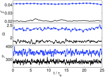
Figure 1: (Color online) (a) Plots versus time $t/\tau_{e}$ of the total kinetic energy $\mathcal{E}$ of the fluid (top panel), the enstrophy $\Omega$ (middle panel), and the palinstrophy $\mathcal{P}$ (bottom panel) for $c=0$ (upper curve, blue circles for run ${\tt R7}$) and $c=0.4$ (lower curve, black line for run ${\tt R7}$); (b) log-log (base 10) plots of the energy spectra $E(k)$ versus $k$ for $c=0.2$ (red triangles for run R10) and $c=0$ (blue circles for run R10); (c) polymer contribution to the scale-dependent viscosity $\Delta\nu(k)$ versus $k$ for $c=0.2$ (red line for run R10), $\Delta\nu(k)=0$ is shown as black dotted line; and (d) energy flux $\Pi(k)$ versus $k$ for $c=0.2$ (red dotted line for run R10) and $c=0$ (blue line for run R10).

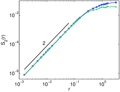
Figure 2: (Color online) (a) Plots of the second-order velocity structure function $S_{2}(r)$ versus $r$ for $c=0$ (blue circle for run R7) and $c=0.2$ (green asterisks for run R7); the line with slope $2$ is shown for comparison; (b) plots of the hyeprflatness $F_{6}(r)$ versus $r$ for $c=0$ (blue circles for run R7) and $c=0.2$ (green asterisks for run R7).

We have tested explicitly that the statistical properties we measure do not depend on the resolutions we use for our DNS. We check this both by increasing and decreasing this resolution. Indeed, our DNS uses the highest resolution that has been attempted so far for this problem (it uses 256 times as many collocation points as those in Ref. berti08 ). Furthermore, the Kurganov-Tadmor shock-capturing scheme that we use controls any dispersive errors, because of sharp gradients in the polymer-conformation tensor, as in similar three-dimensional studies perlekar06 ; vai03 .

We maintain a constant energy-injection rate $E_{inj}\equiv\langle{\bf F_{u}}\cdot\bf u\rangle$ with $F_{\omega}=\nabla\times{\bf F_{u}}$; the system attains a nonequilibrium, statistically steady state after $\simeq 2\tau_{e}-3\tau_{e}$, where the box-size eddy-turnover time $\tau_{e}\equiv{\mathbb{L}}/u_{rms}$ and $u_{rms}$ is the root-mean-square velocity.

In addition to ${\boldsymbol{\omega}}({\bf x},t)$, ${\bf\psi}({\bf x},t)$, and ${\cal C}({\bf x},t)$ we obtain ${\bf u(\bf x},t)$, the fluid-energy spectrum $E(k)\equiv\sum_{k-1/2<k^{\prime}\leq k+1/2}k^{\prime 2}\langle|\hat{\bf\psi}({\bf k^{\prime}},t)|^{2}\rangle_{t}$, where $\langle\rangle_{t}$ indicates a time average over the statistically steady state, the total kinetic energy  ${\mathcal{E}}(t)\equiv\langle\frac{1}{2}|{\bf u(\bf x},t)|^{2}\rangle_{\bf x}$, enstrophy  ${\Omega}(t)\equiv\langle\frac{1}{2}|\boldsymbol{\omega}({\bf x},t)|^{2}\rangle_{\bf x}$, and palinstrophy  ${\mathcal{P}}(t)\equiv\langle\frac{1}{2}|{\nabla\times\boldsymbol{\omega}}({\bf x},t)|^{2}\rangle_{\bf x}$, where $\langle\rangle_{\bf x}$ denotes a spatial average, the PDF of scaled polymer extensions $P(r_{P}/L)$, the PDFs of $\omega^{2}$, $\sigma^{2}$, and $\Lambda=(\omega^{2}-\sigma^{2})/8$, where $\sigma^{2}\equiv\sum_{ij}\sigma_{ij}\sigma_{ij}$, and $\sigma_{ij}\equiv\partial_{i}u_{j}+\partial_{j}u_{i}$, the PDF of the Cartesian components of $\bf u$, and the joint PDF of $\Lambda$ and $r_{P}^{2}$. We obtain the isotropic part of order-$p$, structure function $S_{p}(r)$ from longitudinal velocity increments as described in Ref perlekar09 . We concentrate on $S_{2}(r)$ and the hyperflatness $F_{6}(r)\equiv S_{6}(r)/[S_{2}(r)^{3}]$; the latter is a measure of the intermittency at the scale $r$.

III Results

In Fig. (1a) we show how ${\mathcal{E}}(t)$ (top panel), $\Omega(t)$ (middle panel), and ${\mathcal{P}}(t)$ (bottom panel) fluctuate about their mean values $\langle{\mathcal{E}}(t)\rangle_{t}$, $\langle\Omega(t)\rangle_{t}$, and $\langle{\mathcal{P}}(t)\rangle_{t}$ for $c=0$ (pure fluid) and $c=0.4$. Clearly, $\langle{\mathcal{E}}(t)\rangle_{t}$, $\langle\Omega(t)\rangle_{t}$, and $\langle{\mathcal{P}}(t)\rangle_{t}$ decrease as $c$ increases. Thus, polymers increase the effective viscosity of the solution; but this naïve conclusion has to be refined, as will be shown later, because the effective viscosity depends on the length scale procacciapoly ; perlekar06 ; perlekar10 .

In Fig. (2a), we plot $S_{2}(r)$ versus $r$ for $c=0$ (blue circles and run $\tt R7$) and $c=0.2$ (green asterisks and run $\tt R7$); the dashed line, with slope 2, is shown to guide the eye; this slope agrees with the $S_{2}(r)\sim r^{2}$ form that we expect, at small $r$, by Taylor expansion. At large values of $r$, $S_{2}(r)$ deviates from this $r^{2}$ behavior, more so for $c=0.2$ than for $c=0$, in accord with experiments  jun06 . Plots of $F_{6}(r)$ versus $r$ (Fig. (2b)), for $c=0$ (blue circles) and $c=0.2$ (green asterisks and run $\tt R8$), show that, on the addition of polymers, small-scale intermittency decreases as $c$ increases.

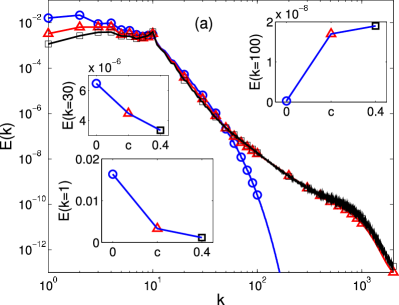
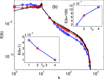
Figure 3: (Color online) (a) Log-log (base 10) plots of the energy spectra $E(k)$ versus $k$ for $c=0$ (blue circles for run ${\tt R6}$), $c=0.2$ (red triangles for run ${\tt R6}$), and $c=0.4$ (black squares for run ${\tt R6}$); plots of $E(k)$ versus $c$ for $\mathcal{W}i=1.53$ and $k=1$ (left bottom inset), $\mathcal{W}i=1.53$ and $k=30$ (left top inset), and $\mathcal{W}i=1.53$ and $k=100$ (right top inset); (b) log-log (base 10) plots of $E(k)$ versus $k$ for $\mathcal{W}i=2.26$ (blue circles for run $\tt R2$), $\mathcal{W}i=4.52$ (red triangles for run $\tt R2$), and $\mathcal{W}i=9.04$ (black squares for run $\tt R2$); plots of $E(k)$ versus $\tau_{P}$ for $c=0.4$ and $k=1$ (left bottom inset) and $c=0.4$ and $k=100$ (right top inset).

In Fig. (3a), we show how $E^{p}(k)$ changes, as we increase $c$ : at low and intermediate values of $k$ (e.g., $k=1$ and $30$, respectively), $E^{p}(k)$ decreases as $c$ increases; but, for large values of $k$ (e.g., $k=100$), it increases with $c$. Figure (3b) shows how $E^{p}(k)$ changes, as we increase $\tau_{P}$ with $c$ held fixed at $0.1$. At low values of $k$ (e.g., $k=1$), $E^{p}(k)$ decreases as $\tau_{P}$ increases; but for large values of $k$ (e.g., $k=100$) it increases with $\tau_{P}$.

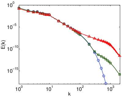
Figure 4: (Color online) (a) Log-log (base 10) plots, for $c=0.2$ and $\mathcal{W}i=2.91$, of $E(k)$ versus $k$ for $L=100$ (red triangles for run $\tt R8$) and $L=10$ (green asterisks for run R9); and $E(k)$ for $c=0$ (blue circles for run $\tt R8$); (b) plots, for $L=100$ (red triangles for run $\tt R8$) and $L=10$ (green asterisks for run R9), of the scale-dependent correction to the viscosity $\Delta\nu(k)$ versus $k$.

In Fig. (4a) we give plots, for $c=0.1$, of the spectra $E^{p}(k)$ for $L=100$ (red triangles and run $\tt R8$) and $L=10$ (green asterisks and run $\tt R9$); for comparison we also plot $E^{f}(k)$ for $c=0$; as $L$ increases, the difference between $E^{p}(k)$ and $E^{f}(k)$ increases at large values of $k$. We see that the larger the value of $L$ the more pronounced is the rise of the large-$k$ tail of $E^{p}(k)$ (cf. the plots in Fig. (4a) with red triangles and green asterisks for $L=100$ and $L=10$, respectively).

We can understand these trends qualitatively by noting that, even at maximal extension, the size of a polymer is $\leq\eta$ (the dissipation scale). Thus, the polymers stretch at the expense of the fluid energy, which cascades from the intermediate length scales to dissipative scales; this leads to a reduction of $E(k)$ at the values of $k$ that correspond to these intermediate scales. As the polymers relax, they feed energy to the fluid at the deep-dissipation, i.e., large-$k$, scales; this leads to an enhancement in the tail of $E(k)$ at large values of $k$. The reduction of energy in the inverse-cascade, low-$k$ regime can be understood by noting that polymers enhance the overall, effective viscosity of the fluid. Indeed, in the limit $\tau_{P}\to 0$, $\nu\nabla^{2}{\bf u}+\frac{\mu}{\tau_{P}}\nabla\cdot{f(r_{P})C}\to(\nu+\mu)\nabla^{2}{\bf u}$  bird87 .

To understand quantitatively the effect of polymers on $E(k)$, in different regimes of $k$, we must compare the fluid-energy spectra, with and without polymers (Fig. (1b)). This leads us naturally to define procacciapoly ; perlekar06 ; perlekar10 the effective, scale-dependent viscosity $\nu_{e}(k)\equiv\nu+\Delta\nu(k)$, with

$$\Delta\nu(k) \equiv -\mu\sum_{k-1/2<k^{\prime}\leq k+1/2}\frac{{\bf u}_{\bf k^{\prime}}\cdot(\nabla\cdot{\cal J})_{\bf-k^{\prime}}}{[\tau_{P}{k}^{2}E^{p}(k)]}$$ (6)

and $(\nabla\cdot{\cal J})_{\bf k}$ the Fourier transform of $\nabla\cdot{\cal J}$. Figure (1c) shows that $\Delta\nu(k)>0$ for $k<30$, where $E^{p}(k)<E^{f}(k)$, whereas, for large values of $k$, $\Delta\nu(k)<0$, where $E^{p}(k)>E^{f}(k)$; the superscripts $f$ and $p$ stand, respectively, for the fluid without and with polymers. To understand this dependence on $L$ we plot, in Fig. (4b), the scale-dependent viscosity $\Delta\nu$ for these two representative values, namely, $L=100$ (red triangles and run $\tt R8$) and $L=10$ (green asterisks and run $\tt R9$). We find that $\Delta\nu$ is positive and higher for $L=100$, at small values of $k$, than its counterpart for $L=10$; this explains why $E^{p}(k)$ is smaller for $L=100$ than for $L=10$ at small $k$. For large values of $k$, $\Delta\nu$ is more negative for $L=100$ than for $L=10$, so $E^{p}(k)$ is larger for $L=100$ than for $L=10$. Note that $\Delta\nu(k)$ changes its sign, from positive to negative, at a smaller value of $k$ for $L=100$ than for $L=10$; therefore, the large-$k$ tail of $E^{p}(k)$ rises above that of $E^{f}(k)$ at a smaller value of $k$ for $L=100$ than for $L=10$. By using $\nu_{e}(k)$, which we obtain from our NS+FENE-P run $\tt R7$, we carry out a DNS of the NS equation with $\nu$ replaced by $\nu_{e}(k)$; in Fig. 5 we present plots of the energy (left panel), energy spectra (middle panel), PDFs of $\Lambda$ (right panel and Fig. 8), to compare the results of this DNS with those of run $\tt R7$ (NS+FENE-P); the good agreement of these results shows that the NS equation with the scale-dependent viscosity $\nu_{e}(k)$ captures the essential effects of polymer additives on fluid turbulence in run $\tt R7$ (NS+FENE-P). The form of our effective viscosity indicates that, at large length scales, in addition to the friction, polymers also provide a dissipative mechanism. By contrast, at small length scales, polymers inject energy back into the fluid.

Figure (1d) shows the suppression, by polymer additives, of $\Pi(k)=\int_{k^{\prime}}^{\infty}T(k^{\prime})dk^{\prime}$, where $T(k)=\int\hat{u_{i}}({\bf-k})P_{ij}({\bf k})\widehat{({\bf u}\times\boldsymbol{\omega})_{j}}({\bf k}){d\Omega}$ and $P_{ij}({\bf k})=\delta_{ij}-\frac{k_{i}k_{j}}{k^{2}}$. The suppression of the spectrum in the small-$k$ régime, which has also been seen in experiments  amarouchene02 and low-resolution DNS (Fig. (4.12) of Ref. mussachiothesis ), signifies a reduction of the inverse cascade; the enhancement of the spectrum in the large-$k$ régime leads to the reduction in $\Omega$ and ${\mathcal{P}}$ shown in Fig. (1a); to identify this enhancement unambigouosly requires the run $\tt R10$, which is by far the highest-resolution DNS of Eqs. (1)-(3) (with $256$ times more collocation points than, say, Ref. berti08 ).

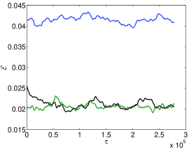
Figure 5: (Color online) Plots with comparisons of the energy (a), energy spectra (b), and the PDF of $\Lambda$ (c) from our DNS of the NS equations with the scale-dependent viscosity $\nu_{e}(k)$ (black squares) and from the NS+FENE-P run $\tt R7$ (green stars). (We calculate $\nu_{e}(k)\equiv\nu+\Delta\nu(k)$ by substituting our data from run $\tt R7$ into Eq. (6).) For reference, we also give plots of all these quantities for the NS equation with conventional, scale-independent viscosity (blue circles).

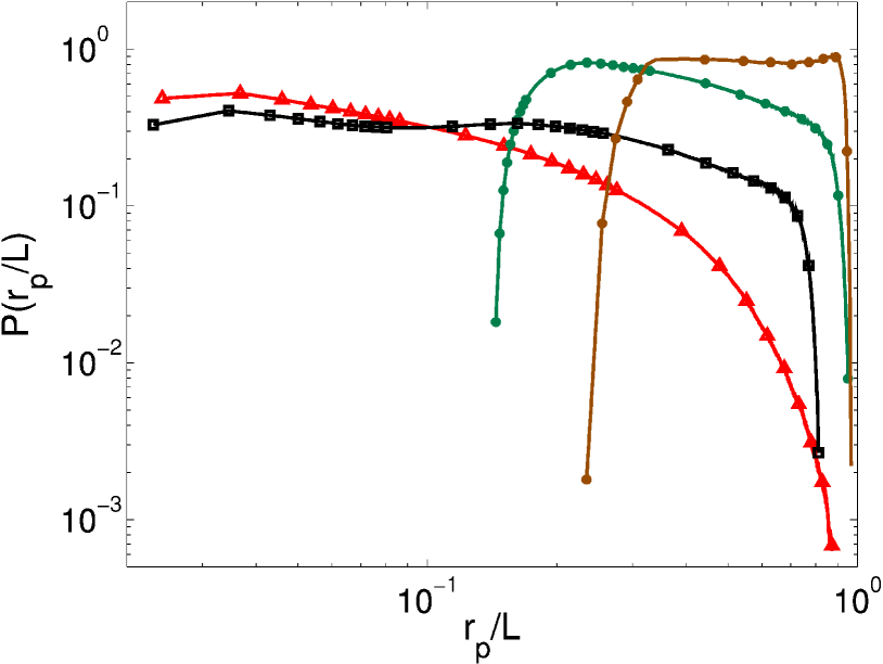
Figure 6: (Color online) PDFs of the scaled polymer extensions $P(r_{P}/L)$ versus $r_{P}/L$ for $c=0.1$ and $L=100$ (red triangles for run R8), $c=0.4$ (black squares for run $\tt R8$), $c=0.1$ and $L=10$ (green asterisks for run $\tt R9$), and $c=0.1$ and $L=6$ (brown dots for run $\tt R1$).

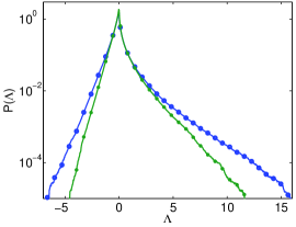
Figure 7: (Color online) Probability distribution functions (PDFs) of (a) the Okubo-Weiss parameter $\Lambda$ for run $\tt R7$ , (b) $\sigma^{2}$ for run $\tt R7$, and (c) $\omega^{2}$ [inset: a PDF of the velocity component $u_{x}$ for $c=0$ (blue circles for run $\tt R7$) with a fit $(1/2)\exp(-u_{x}^{2}/12.5)$ (blue solid line), and for $c=0.2$ (green asterisks for run $\tt R7$) with a fit $(1/2.65)\exp(-u_{x}^{2}/20)$ (green solid line) (note that the addition of polymers reduces the rms value of $u_{x}$)].

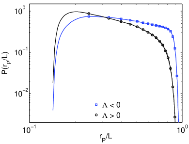
Figure 8: (Color online) (a) Conditional PDF of ($r_{P}/L$) conditioned on $\Lambda$ for run $\tt R9$), (b) a pseudocolor plot of $\Lambda$ superimposed on a contour plot of $r_{P}^{2}$ for run $\tt R10$.

We now plot the PDF $P(r_{P}/L)$ versus $r_{P}/L$ in Fig. (6) for $c=0.1$ and $L=100$ (red triangles and run $\tt R8$), $c=0.4$ and $L=100$ (black squares and run $\tt R8$), and $c=0.1$ and $L=10$ (green asterisks and run $\tt R9$). The extension of the polymers is bounded between $\sqrt{2}\leq r_{P}\leq L$. The lower bound, $r_{P}=\sqrt{2}$, corresponds to polymers in a coiled state; near the upper bound, with $r_{P}\sim L$, the polymers are in a stretched state. In Fig. (6), we show that $P(r_{P}/L)$ shows a distinct, power-law regime, with exponents that depends on $c,L,$ and $Wi$. As $Wi$ increases, this exponent can go from a negative value to a positive value, thus signalling a coil-stretch transition.

In Figs. (7a), (7b), and (7c) we present PDFs of $\Lambda$, $\sigma^{2}$, and $\omega^{2}$, respectively, for $c=0$ (blue circles and run $\tt R7$) and $c=0.2$ (red triangles and run $\tt R7$) to show that the addition of polymers suppresses large values of $\Lambda$, $\sigma^{2}$, and $\omega^{2}$. If we make scaled plots of PDFs such as $P(\Lambda/\Lambda_{rms})$, then they fall on top of each other for different values of $c$; this also holds for $P(\sigma^{2}/\sigma^{2}_{rms})$ and $P(\omega^{2}/\omega^{2}_{rms})$. The inset of Fig. (7c) shows that the PDF of any Cartesian component of u is very close to a Gaussian.

The Fig.(8a) shows a conditional PDF of ($r_{P}/L$) conditioned on $\Lambda$ for run $\tt R9$; this illustrates that polymers stretch predominantly in strain-dominated regions; this is evident very strikingly in Fig. (8b), which contains a superimposition of contours of $r_{P}^{2}$ on a pseudocolor plot of $\Lambda$ (for a video sequence of such plots see suppmat ).

IV Conclusions

We have carried out the most extensive and high-resolution DNS of 2D, homogeneous, isotropic fluid turbulence with polymer additives. We have used the incompressible, 2D NS equation with air-drag-induced friction and polymer additives; the latter have been modelled by using the finitely-extensible-nonlinear-elastic-Peterlin (FENE-P) model for the polymer-conformation tensor. We find that the inverse-cascade part of the energy spectrum in 2D fluid turbulence is suppressed by the addition of polymers. We demonstrate, for the first time, that the effect of polymers on the forward-cascade part of the fluid energy spectrum in 2D is (a) a slight reduction at intermediate wave numbers and (b) a significant enhancement in the large-wave-number range, as in 3D; these features are resolved unambiguously by our high-resolution DNS. In addition, we find dissipation-reduction-type phenomena perlekar06 ; perlekar10 : polymers reduce the total fluid energy and energy- and mean-square-vorticity- or enstrophy-dissipation rates. However, as we have emphasized above, dissipation reduction is not the only notable effect of polymer additives; our extensive, high-resolution DNS of 2D fluid turbulence with polymer additives yields good qualitative agreement, in the low-$k$ régime, with the fluid-energy spectra of Ref. amarouchene02 , and the $S_{2}(r)$ of Ref. jun06 . In addition, our study obtains new results and insights that will, we hope, stimulate new experiments, which should be able to measure (a) the reduction of $\langle\mathcal{E}(t)\rangle_{t}$, $\langle\Omega(t)\rangle_{t}$, and $\langle{\mathcal{P}}(t)\rangle_{t}$ (Fig.(1a)), (b) the modification of $E^{p}(k)$ at large $k$ (Fig.(1b)), (c) the $c$, $\tau_{P}$ and $L$ dependences of $E^{p}(k)$ (Figs.(3a),(3b) and (4a)), (d) the PDFs of $(r_{P}/L)$, $\Lambda$, $\sigma^{2}$, and $\omega^{2}$, (e) the stretching of polymers in strain-dominated regions (Fig. (8b)), and (f) the suppression of $F_{6}(r)$ at small $r$ (Fig. (2)).

Two-dimensional fluid turbulence with polymer additives has been studied in channel flows, both in experiments kellayexpt and via DNS kellaydns ; this DNS study uses the Oldroyd-B model, which does not have a maximal-polymer-extension length and is, therefore, less realistic than the FENE-P model we use. These studies obtain energy spectra and second-order structure functions that are qualitatively similar to those we obtain, except at small length scales, which are not resolved in these channel-flow studies. This shows, therefore, that energy spectra and structure functions, obtained far away from walls, are not affected significantly by the walls. Thus, our studies are relevant to the bulk parts of wall-bounded flows too.

V Acknowledgments

We thank D. Mitra for discussions, CSIR, UGC, DST (India), and the COST Action MP006 for support, and SERC (IISc) for computational resources. AG thanks the grant from European Research Council under the European Community’s Seventh Framework Programme (FP7/2007-2013)/ERC Grant Agreement N. 279004.

References

- (1) B.A. Toms, in Proceedings of the International Congress on Rheology, Vol. II (North-Holland, Amsterdam, 1949), p. 135; J. Lumley, J. Polym. Sci. Macromol. Rev. 7, 263 (1973).
- (2) P. Virk, AIChE 21, 625 (1975).
- (3) J.W. Hoyt, Trans. ASME J. Basic Eng. 94:25–5 (1972).
- (4) E. van Doorn, C.M. White, and K.R. Sreenivasan, Phys. Fluids 11, 237 (1999).
- (5) C. Kalelkar, R. Govindarajan, and R. Pandit, Phys. Rev. E 72, 017301 (2005).
- (6) R. Benzi, E. S. C. Ching, and I. Procaccia, Phys. Rev. E 70, 026304 (2004); R. Benzi, N. Horesh, and I. Procaccia, Europhys. Lett., 68, 310 (2004).
- (7) P. Perlekar, D. Mitra, and R. Pandit, Phys. Rev. Lett. 97, 264501 (2006).
- (8) P. Perlekar, D. Mitra, and R. Pandit, Phys. Rev. E. 82, 066313 (2010).
- (9) W.-H. Cai, F.-C. Li and H.-N. Zhang, J. Fluid Mech. 665, 334 (2010).
- (10) F. De Lillo, G. Boffetta, S. Musacchio, Phys. Rev. E. 85, 036308 (2012).
- (11) N. Ouellette, H. Xu, and E. Bodenschatz, J. Fluid Mech. 629, 375 (2009).
- (12) R. Benzi, E. S. C. Ching, and C. K. Wong, Phys. Rev. E. 89, 053001 (2014).
- (13) T. Watanabe, and T. Gotoh, Phys. Fluids. 26, 035110 (2014).
- (14) Y. Amarouchene and H. Kellay, Phys. Rev. Lett. 89, 104502 (2002).
- (15) H. Kellay, Phys. Rev. E. 70, 036310 (2004).
- (16) Y. Jun, J. Zhang, and X-L Wu, Phys. Rev. Lett. 96, 024502 (2006).
- (17) S. Musacchio, Ph.D. thesis, Department of Physics, University of Torino, (2003).
- (18) S. Berti, et al., Phys. Rev. E, 77, 055306(R) (2008).
- (19) G. Boffetta, A. Celani, and S. Musacchio, Phys. Rev. Lett. 91, 034501 (2003); G. Boffetta, A. Celani, and A. Mazzino, Phys. Rev. E 71, 036307 (2005).
- (20) Y. L. Xiong, C. H. Brueneua, and H. Kellay, Europhys. Lett. 95, 64003 (2011).
- (21) G. Boffetta and R. Ecke, Annu Rev Fluid Mech. 44, 427-451 (2012); R. Pandit, P. Perlekar, and S. S. Ray, Pramana-Journal of Physics,73, 157(2009).
- (22) P. Perlekar, and R. Pandit, New Journal of Physics, 11, 073003 (2009).
- (23) A. Okubo, Deep-Sea Res. Oceanogr. Abstr. 17 445 (1970); J. Weiss, Physica D (Amsterdam) 48, 273 (1991).
- (24) T. Vaithianathan and L. R. Collins, J. Comput. Phys. 187, 1 (2003).
- (25) A. Kurganov and E. Tadmor, J. Comput. Phys. 160, 241–22 (2000).
- (26) http://www.fftw.org
- (27) R.B. Bird, C.F. Curtiss, R.C. Armstrong, O. Hassager, Dynamics of Polymeric Liquids - Volume 2: Kinetic Theory, 2nd Edition John Wiley, New York (1987).
- (28) See Supplemental Material at URL for the Video sequence showing pseudocolor plots of the Okubo-Weiss parameter superimposed on contour plots of , which measures the polymer extension. Note that polymers stretch predominantly in the strain-dominated regions of the flow.