Measurement of the beauty of periodic noises

Abstract

In this article indicators to describe the “beauty” of noises are proposed. Rhythmic, tonal and harmonic suavity are introduced. They give a characterization of a noise in terms of rhythmic regularity (rhythmic suavity), of auditory pleasure of the “chords” constituting the signal (tonal suavity) and of the transition between the chords (harmonic suavity). These indicators have been developed for periodic noises typically issued from rotating machines such as engines, compressors… and are now used by our industrial customers since two years.

I Introduction

In the industry, we often have to improve a noisy environment. The first way, after having identified the sources, consists of lowering the noise level arriving to the user. Hovewer nowadays, this is not sufficient. Conforming to acoustic standards, even drastic ones, does not imply customer’s satisfaction. Indeed, to endure a noise during hours, even with a moderate intensity, is only possible if this noise has a certain quality, a certain “beauty”.

Moreover, we face more and more emergency situations, which means that solutions have to be developed and installed very quickly. We cannot use sequential trials nor ask customers about their feelings. We have to directly furnish the “right” solution in terms of noise level as well as sound comfort (sound beauty). This is why it is necessary to be able to characterize this beauty in some sense.

In this article, we present several indicators, each one describing the sound beauty according to a point of view. These indicators, defined as values between 0 (bad) and 1 (perfect), can then be combined into a global indicator of the considered noise.

To approach the subject of the beauty of a noise is fundamentally different from that for example the music. This is why no reference is made ​​to works of classical psychoacoustics. We want to emphasize that we only deal with noises, and more precisely with “neutral” noises: a neutral noise is a noise to which no cultural nor emotional component is attached. For example, the noise of a car engine is not neutral, because its perception is clearly related to cultural and emotional factors. But noises of an air conditioner, of an industrial compressor or of the engine of a mechanical tool are neutral.

II Stage 1 (optional): determination of “cycles” in the acoustic signal

In music (played by musicians, not generated by computers), time between two successive pulses cannot generally be less than 20 ms (even if smaller values can be found in more contemporary musical forms). But GreenGreen (1971) and RoadsRoads (1991) showed that events separated by only 1 ms can be detected by human ears.

Therefore, we do not impose any minimum duration of cycles that we study. This is especially true for periodic signals, where even a very small part of the signal is important because it is repeated again and again.

Since we study periodic signals, we must be able to isolate a signal cycle to examine it in detail.

Fig. 1 presents a typical temporal signal of a periodic phenomenon.

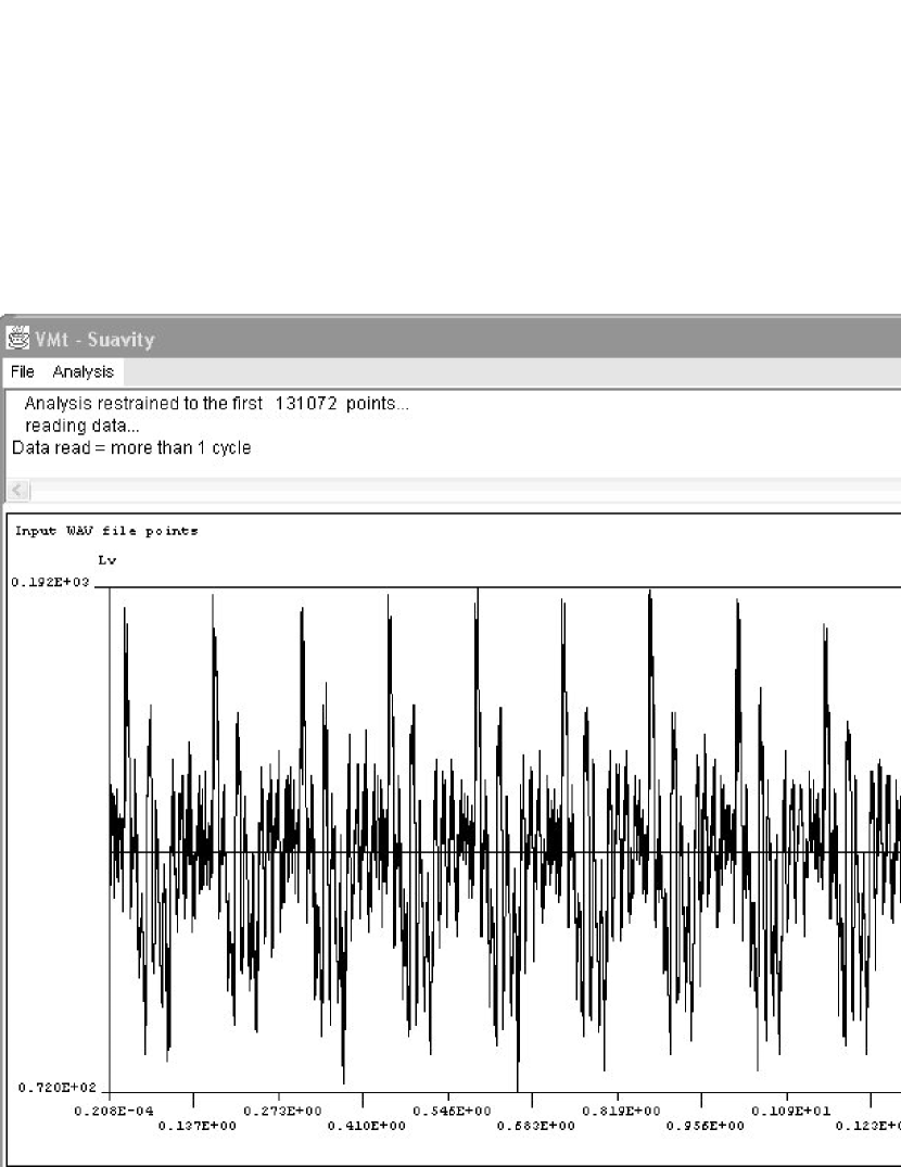
Figure 1: Typical temporal recording of a periodic signal

Studied signals (cyclic noise emitted by rotating machines) have the distinction of having an emerging component at each cycle. The algorithm exploits this property: a first approximation of the cycle time is obtained by studying the lowest frequencies of the spectrum. This approximation is then refined by the study of the temporal signal. This gives excellent results, as illustrated by industrial examples presented at the end of the article.

If this algorithm is not adapted to the kind of studied signal, we suppose that a cycle is extracted using another method (or manually), and in following stages, we consider only one cycle of the signal.

III Stage 2: Rhythmic suavity

This indicator represents the rhythmic regularity of an acoustic signal, and is based on a temporal analysis of the signal. For example, an engine can rotate in a uniform way or not (without taking into account the sound it produces). This feeling of regularity or of irregularity is already a part (a component) of the beauty of the acoustic signal. In order to define it, we propose to find the pulses within the considered acoustic signal, i.e. to find where acoustic events occur. The rhythmic suavity will be defined as the number of acoustic events divided by the total number of pulsations within the whole acoustic signal.

Software having a “beat finder” function often use a dynamical approach (in a musical sense) in order to represent the notion of beginning (or ending) of a note. Pulses are located where voices come into play: a slope greater than a given threshold is hunted in the temporal signal, as for example in Audacitybib (006) software. This notion can also be studied in a spectral way, as for example, in AudioSculptLithaud et al. (008) software.

For short periodic signals (which are our concern), methods based on the spectrum derivative or variation are not adapted because notions such as beginning or ending of notes do not exist: the signal is too smooth (compared to music), and to lower the threshold leads to very unstable results. Smoothing methods (as windowed average) applied to the signal leads to the same kind of threshold problems.

Implemented algorithm, illustrated in Fig. 2, is based on the following ideas: The studied signal (one cycle) is divided into $n$ equal ranges. The variation direction of mean values other each range is studied to detect when it changes from decreasing or constant to increasing (which corresponds to the notion of beginning of note); The exact inflexion point is determined as the minimum in the temporal signal corresponding to the inflexion range and on the two adjacent ranges.

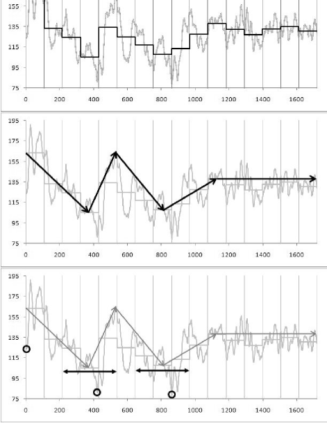
Figure 2: Implemented “beat finder” algorithm: 1) one cycle (temporal signal), 2) mean values of signal within the 16 ranges, 3) variation of averages, 4) ranges (horizontal arrows) in which the minimum (encircled) represents a pulse.

Knowing these instants when acoustic events occur (called pulses), it is obvious to find the minimal pulsation, so that each pulse and the total duration of a cycle are a multiple of this pulsation, and hence to reach the rhythmic suavity. With such a definition, the rhythmic suavity is a real number lying between 0 and 1.

IV Stage 3: Tonal suavity

We call “chord” the frequency content of the part of the signal contained between two successive pulses. A chord is constituted by a certain number of “notes” corresponding to frequencies present in the chord.

A method derived from Euler’s work will be used to compute the ”beauty” of each chord relatively to the tonal centre of the signal.

The tonal suavity for the whole acoustic signal will be obtained by balancing the beauty of each chord with respect to its duration.

IV.1 Determination of the tonal centre

When considering music, it is easy to determine the tonal centre (i.e. the tonic) with the score.

But, when considering a noise, this task is not so simple. Nevertheless, there are many ways to determine an “equivalent note” or a tonal centre of an acoustic signal.

It is possible to use prominent frequency methods: both “Tone to noise ratio” as defined by standardsbib (2002, 1995), and “Prominence ratio”defined by standardbib (1995) can be used. For these methods, a tone is said to be prominent if it fulfills some criteria within the critical band centered at the frequency of the tone. When multiples tones are in the same critical band, prominence ratio is more effective; and when multiple tones exist in adjacent critical bands (strong harmonics), tone-to-noise ratio should be preferred. From these frequencies, the most emerging one can be chosen as the tonal centre.

In this work, we define the tonal centre as the fundamental frequency of the signal, since it is generally a value of interest when considering a periodic signal (at least from a mechanical and energetic point of view). It means that we retain the lowest frequency peak in the signal. For this purpose, a Bartlett function is used in the FFT in order to favor lower frequencies.

In the following, $f_{0}$ will denote the frequency corresponding to the tonal centre of the signal.

IV.2 Tonal suavity

Tonal suavity will be calculated using a modified version of Euler’s worksEuler (1739, 1766, 1773). This approachEuler (1772) is primarily a physicist’s approach, and is close to Helmholtz’s work. Besides, the classification of beauty of chords constituted by only two notes are exactly the same for EulerEuler (1739) and Helmholtzvon Helmholtz (1877).

This modified version of Euler’s work has a major advantage: once the classification scale of the beauties of chords constituted by two notes is determined, then it can be extended to chords constituted by any number of notes spread over any number of octaves.

A chord (previously defined as the frequency content between two successive pulses) is constituted by $n$ notes. We shall denote $f_{1}$, $f_{2}$, …, $f_{n}$ the $n$ frequencies corresponding of these $n$ notes of the chord ($f_{0}$ denoting the frequency of the tonal centre of the signal as defined previously).

IV.3 Euler’s work

Euler defines a “degree of sweetness”, a kind of “easiness”, which is his indicator: the less this indicator, easier to perceive the order between notes, or equivalently more beautiful the sound.

Euler’s theory can be summarized as follows:

• A note is replaced by a number lying between 0 (unisson) and 12 (octave) and corresponding to its interval to the tonal centre.

• The “exponent” of a chord is defined as the LCM (least common multiple) of the ratios of frequencies related to the tonal centre of the signal: exponent = LCM($f_{1}/f_{0},...,f_{n}/f_{0}$). In order to calculate LCM, we have to manage only integers. Hence, if ratios $f_{i}/f_{0}$ are not all integers, they are all multipled by an adequate coefficient.

• The exponent is then decomposed in product of primes:

  $$\text{exponent}_{\text{chord}}=\prod_{k}p_{k}^{j_{k}}$$ (1)

  where $k$ is the number of primes $p_{k}$ necessary to perform this decomposition and $j_{k}$ their exponent. This prime decomposition is given in table 1. Some examples are proposed in table IV.3.

• The easiness of a chord is computed from the previous prime decomposition as:

  $$\text{easiness}_{\text{chord}}=1+\sum_{k}j_{k}(p_{k}-1)$$ (2)

  The result is written using roman numbers in table IV.3.

To illustrate the methods in this article, we use music, and more precisely, we use C Major (no key signature). Hence a chord whose bass is C will be represented by the number 1 (because it is also the tonal centre). A note C one octave higher will be represented by the number 2 (because its frequency is the double of the one of tonal centre). A note F a fourth higher than the tonal centre will be represented by 4/3 which represents the ratio of its frequency to the tonal centre. These ratios between notes heights are given in table 1.

Table 1: Euler’s music scale and easiness

interval	$i$	Prime decomposition	easiness
unison	0	1	1
minor $\text{2}^{\text{nd}}$	1	$2^{4}.3^{-1}.5^{-1}$	11
Major $\text{2}^{\text{nd}}$	2	$2^{-3}.3^{2}$	8
minor $\text{3}^{\text{rd}}$	3	$2.3.5^{-1}$	8
Major $\text{3}^{\text{rd}}$	4	$2^{-2}.5$	7
$\text{4}^{\text{th}}$	5	$2^{2}.3^{-1}$	5
aug. $\text{4}^{\text{th}}$	6	$2^{-5}.3^{2}.5$	14
$\text{5}^{\text{th}}$	7	$2^{-1}.3$	4
minor $\text{6}^{\text{th}}$	8	$2^{3}.5^{-1}$	8
Major $\text{6}^{\text{th}}$	9	$3^{-1}.5$	7
minor $\text{7}^{\text{th}}$	10	$2^{4}.3^{-2}$	9
Major $\text{7}^{\text{th}}$	11	$2^{-3}.3.5$	10
octave	12	$2$	2

Some examples of numbering of intervals are given in table IV.3.

Table 2: Numbering of some chords according to Euler

chord	cj	cf	ceg
ratio	2	4/3	5/4 and 3/2
coefficient	1	3	4
tonal centre	c	160 F	160 C
	unchanged	modified	modified
exponent	LCM(1;2)=2	LCM(3;4)=12	LCM(4;5;6)
	$=2^{1}$	$=2^{2}.3$	$=2^{2}.3.5$
easiness	1+1 = II	1+2+2 =IV	1+2+2+4 =IX

IV.4 Modification, extension

Concerning Euler’s work, we can make the following remarks:

• In order to have only natural numbers, it is necessary to multiply the approximations of $f_{i}/f_{0}$ ratios according to table 1 by a coefficient. Doing this corresponds to change the tonal centre used to perform the numbering. For example, in second chord of table IV.3, we have to multiply by 3 to have integers. This corresponds to change the C tonal centre by a F tonal centre two octaves lower.

• Nevertheless, insofar as the same coefficient is used to number all the chords of the signal, this has only a relative importance because the numbering is still done with respect to the same note even if it is no more the tonal centre.

Because the fundamental frequency is a value on interest in the industrial cases we face, we do not want to change the tonal centre $f_{0}$ used in the numbering process. It is therefore necessary to modify the approximations of intervals. We have to find a set of primes so that i) it is possible to correctly approximate the powers of twelfth root of 2, ii) having only powers of 2 as denominators and iii) so that easiness obtained for the intervals are classified in the same order of the ones obtained by Euler.

Such an approximation is presented in table 3.

Table 3: Proposed scale and easiness

interval	$i$	Prime decomposition	easiness
unison	0	$1$	1
minor $\text{2}^{\text{nd}}$	1	$2^{-12}.3.5.7.41$	65
Major $\text{2}^{\text{nd}}$	2	$2^{-7}.11.13$	30
minor $\text{3}^{\text{rd}}$	3	$2^{-4}.19$	23
Major $\text{3}^{\text{rd}}$	4	$2^{-6}.3.5$	17
$\text{4}^{\text{th}}$	5	$2^{-8}.7^{3}$	27
aug. $\text{4}^{\text{th}}$	6	$2^{-10}.31.47$	87
$\text{5}^{\text{th}}$	7	$2^{-5}.3^{2}.5$	14
minor $\text{6}^{\text{th}}$	8	$2^{-8}.11.37$	55
Major $\text{6}^{\text{th}}$	9	$2^{-9}.3.17^{2}$	44
minor $\text{7}^{\text{th}}$	10	$2^{-12}.3^{2}.5.7.23$	49
Major $\text{7}^{\text{th}}$	11	$2^{-9}.3.11.29$	50
octave	12	$2$	2

Contrary to Euler, who only used powers of 2, 3 and 5 for the decompositions, we use 2, 3, 5, 7, 11, 13, 17, 19, 23, 29, 31, 37, 41 and 47. Nevertheless, it does not make the computation algorithm more complicated (since prime decomposition is not computed but directly obtained by construction).

Easiness of intervals corresponding to this new decomposition have higher values than Euler’s ones, but globally respect the same order. Some differences can be seen which permit to include Euler’s latest workEuler (1766), and to better take into account some consonances. Spreading values of easiness over a large range yields more distinction in suavity marks.

IV.5 Implemented algorithm

The algorithm is as follows:

1. Determination of the notes constituting a chord:

   From the spectrum of the frequency content corresponding to a chord (signal contained between two acoustic events), we take the $n$ lowest frequency peaks. In developed program, $n\leq 10$, and we stop looking for peaks at $\min(8000~{}\text{Hz},\text{Nyquist frequency})$. We then have $n$ frequencies $f_{n}$ describing the chord.

2. Approximation of the notes of the chord:

   Each frequency $f_{n}$ si approximated by $f_{n}\approx f_{0}.2^{k_{n}}.(\sqrt[12]{2})^{i_{n}}$, where $k_{n}$ is the number of octaves between $f_{n}$ and $f_{0}$ and $i_{n}$ the halftone which is the closest to $f_{n}$ in the considered octave. $(\sqrt[12]{2})^{i_{n}}$ is then replaced by its approximation according to tables 1 or 3.

3. Calculation of the chord’s exponent using equation (1).

4. Calculation of the chord easiness using equation (2).

5. Normalization:

   The lower the easiness, the more the chord is tuneful. On the contrary, we want that the higher the suavity, the more the chord is tuneful. We also want the suavity to lie between 0 and 1.

   We can notice that, for a given chord of $n$ notes: $1\leq\text{easiness}\leq b$ with:

   $$b=o_{n}+a_{n}$$ (3)

   where $o_{n}$ is the upper bound of the number of octaves between the tonal centre and the notes, and $a_{n}$ is the upper bound of the easiness of a chord constituted by $n$ notes.

   $a_{n}$ is the upper bound of equation (2), which is calculated by taken the maximum of each term of the sum:

   $$\begin{array}[]{rl}a_{n}=&1+\sum_{k}\left(\max_{i=1}^{12}j_{i}-\min_{i=1}^{12}(0,j_{i})\right)(p_{k}-1)\\[4.30554pt] =&28\text{~{}if using table~{}\ref{tab-euler}}\\ =&318\text{~{}if using table~{}\ref{tab-VMt}}\end{array}$$ (4)

   If we only consider frequencies between 1 and 10 kHz, then we have a maximum of 14 octaves, which means that $o_{n}=14$ can be used as upper bound.

6. Calculation of the chord suavity:

   Finally, the suavity is defined by:

   $$\text{suavity}_{\text{chord}}=1-\dfrac{\text{easiness}-1}{b-1}$$ (5)

   which lies between 0 and 1 (1 being the better).

7. We finally compute the tonal suavity of the signal as the balanced average of the chords suavity with the duration of the chords:

   $$\text{suavity}_{\text{tonal}}=\sum_{i}\dfrac{\text{suavity}_{\text{chord}_{i}}.\text{duration}_{\text{chord}_{i}}}{\text{total duration of the signal}}$$ (6)

   From its definition, the tonal suavity lies between 0 and 1.

V Stage 4: Harmonic suavity

Harmonic suavity represents the beauty of the transition between two successive chords constituting the signal (plus the last chord followed by the first one for periodic signals). More precisely, harmonic suavity quantifies the beauty of the part of the second chord which does not come from a transformation (belonging to the dihedral group) of the first chord. In this sense, harmonic suavity is related to the rate of change between two acoustic events.

V.1 Existing works

In his work, Euler extends his method in order to determine the beauty of a set of chords or to a whole musical work.

The main idea is the following: the transition between two chords is harmonious if the chord composed of all notes composing the two chords is itself harmonious. By extension, this method could be applied to any number of chords, and hence to a whole musical work.

Two mains objections can be done:

1. Such a method yields a bad mark for transposed chords, as in sequences. Fig 3 exhibits a perfect chord C–E–G, i.e. the C major triad in root position, as the starting chord of a ascending sequence by successive halftones steps. Such a sequence of chords is absolutely not chocking to the ears, because a motif is immediately recognized, which is repeated and transposed. With Euler’s method, we have to take into consideration the chord C–C#–D–D#–E–F–F#–G–G#–A–A#–B, i.e. constituted by all the halftones: this chord has a high easiness or a bad tonal suavity, which perfectly agree with what we hear.

2. Euler does not calculate the beauty of the transition between two chords, but the overall beauty of two (or more) chords considered as a single entity.

ceg ^cf^g d^fh ^dg^h e^gi    c^ceg^gi’d^df^fh^h

Figure 3: An ascending sequence

Another possible way consists to use musicology rules related to the beauty of transition of chords (which is sometimes referred to as “chords in movement”). In this approach, chords are qualified (stables or attractive) and the movement of the bass is analyzed with respect to the degree of the chord (i.e. the position of the bass relatively to the tonal centre). Rules are numerous and delicates. They need an analysis, which can be qualified as syntactic. It is quite impossible to program such rules, especially if we want to number chords having more than 6 notes (which cannot be taken into account)…

V.2 Developed approach

To expose our approach, we continue to explain it using musical example, even if our goal remains the study of industrial noises.

We propose to simplify Euler’s work and combine it with some rule of musical harmony. From musical harmony we keep numbering a chord relatively to its bass, without taking into account octaves. From Euler’s work, we keep the idea according to which the transition between two chords is beautiful if the chord made of all notes of both chords is beautiful. But the method is only applied to the transition between two chords. We only consider a chord relatively to the bass of the previous one (and no more relatively to the tonal centre). Finally, we solve the problem described previously concerning sequences by “suppressing” from the second chord the part that “comes from the first one” (in a sense of transformations belonging to the dihedral group).

As aforementioned, considering a note independently from its octave and relatively to a reference note is equivalent to consider its interval to the reference note. Hence a note can be represented by an elements of the cyclic group $\mathbb{Z}/12\mathbb{Z}$. This cyclic group can be viewed as a regular polygon with $12$ sides, i.e. a dodecagon: the 12 apexes represent the 12 possible halftones for a note (relatively to the bass of the chord). It is depicted in figure Fig. 4.

Figure 4: Dodecagone of the 12 halftones

In the following, notes will be considered independently from octaves: hence C–E–G–C–E is equivalent to C–E–G, i.e. the chord is presented in a “compact” form, as illustrated in figure Fig 5.

Considering a chord made of $p$ notes, it can be represented by a $p$ sided polygon whose apexes belong to the dodecagon. A set $T$ of $p$ values in $\mathbb{Z}/n\mathbb{Z}$, which is equivalent to a $p$ sided polygon whose apexes belong to an $n$ sided polygon, is hence equivalent to a chord constituted by $p$ notes.

For example $T=(0,4,7)$ represents in $\mathbb{Z}/12\mathbb{Z}$ the chord and the polygon depicted in figure Fig 5.

cegjl    ceg   

Figure 5: Representations of a chord (Considered chord / compact chord / corresponding polygon)

Chord $T=(0,4,7)$ correspond to any chord whose second note is located 4 halftones from the first one, and whose third note is located 7 halftones from the first one, the first one being its bass. Such a chord can be C–E–G, as in figure Fig. 5, but also any chord being a transposition of it (see figure Fig. 3).

The dihedral group $D_{n}$ is a group of order $2n$ of plane isometries letting the regular $n$ sided polygon unchanged. $D_{n}$ is made of $n$ rotations and $n$ symmetries. It is generated by two elements: the rotation of one vertice to the next $R_{1}$, and the symmetry with respect to abscissa axe $S_{0}$. The dihedral group $D_{n}$ can hence be written in the form $D_{n}=\{R_{0}=Id,R_{1},...,R_{1}^{n-1},S_{0},R_{1}\circ S_{0},...,R_{1}^{n-1}\circ S_{0}\}$. From a computation point of view, it means that it is sufficient to dispose of $R_{1}$ and $S_{0}$ transformations to be able to browse the entire dihedral group.

From a musical (and a frequential) point a view, we can notice that:

• $R_{0}=Id$ corresponds to a transposition of chord $T$ (as in a sequence);

• $R_{i}$, with $i\geq 1$, corresponds to an inversion of chord $T$ (same notes in a different order) with eventually a transposition;

• $S_{0}$ corresponds to a retrograde of chord $T$ (chord made of the same intervals in the opposite direction) with eventually a transposition;

• $R_{i}\circ S_{0}$, with $i\geq 1$, corresponds to the retrograde of an inversion of chord $T$ with eventually a transposition;

Although each transformation of the dihedral group is different from all others, it does not imply that it exists an unique decomposition of the transformation of a polygon $T$ into a polygon $V$ when $p<n$.

Consider for example chord $T=(0,5,10)$ corresponding to chord C–F–A# and chord $V=(0,2,7)$ corresponding to chord D–E–A. Then $V=R_{2}(T)$, but also $V=S_{0}(T)$.

When several transformations exist, then we choose the one which comes first in the order of transformations, when classified as previously: $D_{n}=\{R_{0}=Id,R_{1},...,R_{1}^{n-1},S_{0},R_{1}\circ S_{0},...,R_{1}^{n-1}\circ S_{0}\}$. It just means that it is easier to hear a transposition, then an inversion, then a retrograde chord, and finally the retrograde chord of an inversion.

Finally, if such a transformation exists, then it is possible to give a “beauty mark” to the transformation. We chose the following marks: 1 for $R_{0}=Id$, 0.9 for $R_{i}$ ($i\geq 1$), 0.8 for $S_{0}$ and 0.7 for $R_{i}\circ S_{0}$ ($i\geq 1$).

V.3 Transformation from a chord to another – dihedral component $\mathscr{D}$ and non congruous component $\mathscr{R}$

Consider chord $T=(0,4,7)$, which may represent the perfect chord C–E–G already presented in figure Fig. 5. Let $V=(0,4,8,9)$ be the chord F–A–C#–D, as illustrated in figure Fig. 6.

It is easy to see that $R_{4}(S_{0}(T))=(0,4,9)=V-\{8\}$.

We call dihedral component, the element of $D_{n}$ allowing to transform $T$ into $V$. It is denoted $\mathscr{D}_{V}(T)$. In this case, the dihedral component is equal to $\mathscr{D}_{V}(T)=R_{4}\circ S_{0}$.

We also define the non congruous component of $V$ relatively to $T$, and we denote it $\mathscr{R}_{V}$, as the remainder when “subtracting” from $V$ its dihedral component $\mathscr{D}_{V}(T)$: it corresponds to the notes belonging to $V$ which are not issued from the transformation of $T$. This definition is quite natural, and we reach: $\mathscr{R}_{V}(T)=+\{8\}$.

Compact writing	In $\mathbb{Z}/12\mathbb{Z}$	Graph	Transformation
ceg	$T=(0,4,7)$
$\downarrow$			$V=\mathscr{D}_{V}(T)+\mathscr{R}_{V}(T)$
fh^j’k	$V=$ $(0,4,8,9)$		$\mathscr{D}_{V}(T)=R_{4}\circ S_{0}$, $\mathscr{R}_{V}(T)=+\{8\}$

Figure 6: Comparison between chords

When no transformation exists between two chords, then the dihedral component $\mathscr{D}=\emptyset$ and the non congruous component $\mathscr{R}$ is equal to the second chord.

V.4 Arithmetic of transformations

Consider a chord $T$ and its successor $V$. As explained, a way to write that $V$ issued from a transformation of $T$ is:

$$V=\mathscr{D}_{V}(T)+\mathscr{R}_{V}(T)$$ (7)

Equation (7) can be seen as a decomposition or a division of $V$ by $T$: $V$ represents the dividend, $T$ the divisor, $\mathscr{D}_{V}(T)$ the quotient and $\mathscr{R}_{V}(T)$ the remainder. This equation could also be written in a modular arithmetic form as: $V\equiv\mathscr{R}_{V}(T)\mod[\mathscr{D}_{V}(T)]$.

Equation (7) can be written in inverse form:

$$T=\mathscr{D}_{T}(V)+\mathscr{R}_{T}(V)$$ (8)

with:

$$\left\{\begin{array}[]{rcl}\mathscr{D}_{T}&=&\mathscr{D}_{V}^{-1}\\ \mathscr{R}_{T}&=&-\mathscr{D}_{V}^{-1}.\mathscr{R}_{V}=-\mathscr{D}_{T}(\mathscr{R}_{V})\end{array}\right.$$ (9)

Since any representative of the dihedral group can only be written as $R_{i}$ or $R_{i}\circ S_{0}$, then (indexes belong to $\mathbb{Z}/n\mathbb{Z}$):

$$\left\{\begin{array}[]{lrcl}\text{if }\mathscr{D}_{V}=R_{i},&\mathscr{D}_{T}&=&R_{-i}\\[4.30554pt] \text{if }\mathscr{D}_{V}=R_{i}\circ S_{0},&\mathscr{D}_{T}&=&S_{0}\circ R_{-i}\\ \end{array}\right.$$ (10)

From equation (10), we can notice that the “beauty mark” of the transformation is the same for the direct and the reverse transformation.

We study again transformation from $T$ into $V$ and from $V$ into $T$ defined by $T=(0,4,7)$ C–E–G and $V=(0,4,8,9)$ F–A–C#–D and illustrated in figure Fig 6. Dihedral and non congruous components can be calculated directly as in previous section, or using equations (9) and (10). Results are reported in figure Fig 7.

ceg	$V=\mathscr{D}_{V}(T)+\mathscr{R}_{V}(T)$ with: $\mathscr{D}_{V}(T)=R_{4}\circ S_{0}$ and $\mathscr{R}_{V}(T)=+\{8\}$ $T=\mathscr{D}_{T}(V)+\mathscr{R}_{T}(V)$ with: $\mathscr{D}_{T}(V)=S_{0}\circ R_{8}$ and $\mathscr{R}_{T}(V)=-\{8\}$	fh^j’k
$T=(0,4,7)$		$V=(0,4,8,9)$

Figure 7: Arithmetic between chords

In this case we have:

• Direct calculation from $T$ to $V$ gives $\mathscr{D}_{V}(T)=R_{4}\circ S_{0}$ and $\mathscr{R}_{V}(T)=\{8\}$,

• Direct calculation from $V$ to $T$ gives $\mathscr{D}_{T}(V)=R_{4}\circ S_{0}$ and $\mathscr{R}_{T}(V)=-\{8\}$.

• Equations (9) and (10) give $\mathscr{D}_{T}(V)=S_{0}\circ R_{-4}=S_{0}\circ R_{8}$ and $\mathscr{R}_{T}(V)=-(S_{0}\circ R_{8})(\{8\})=-S_{0}(\{4\})=-\{8\}$.

The writing of $\mathscr{D}_{T}(V)$ is not unique, but $[R_{4}\circ S_{0}](T)=[S_{0}\circ R_{8}](T)$. The most important point remains that the beauty mark of the dihedral component remains the same, and that both decompositions lead to the same non congruous component $\mathscr{R}_{T}(V)$.

V.5 Harmonic suavity of the transition between two chords

The harmonic suavity, corresponding to the beauty of the transition from chord $T$ to chord $V$, will be calculated as follows:

• If it exists a transformation from $T$ to $V$ then:

  • if the number of notes of $V$ is less or equal to the number of notes of $T$ (i.e. the non congruous component is less or equal to zero), then the harmonic suavity is equal to the mark of the transformation: 1 for $R_{0}$, 0.9 for $R_{i}$ ($i\geq 1$), 0.8 for $S_{0}$ and 0.7 for$R_{i}\circ S_{0}$ ($i\geq 1$);

  • if the number of notes of $V$ is strictly greater than the number of notes of $T$ (i.e. the non congruous component is strictly greater than zero), then we calculate the tonal suavity of chord $\mathscr{R}_{V}(T)$ with respect to the bass of $T$ (i.e. we replace $f_{0}$ by $f_{1}(T)$ in stage 3 algorithm);

• If there is no transformation from $T$ to $V$ then: we calculate the tonal suavity of chord $V$ (we recall that in this case $\mathscr{R}_{V}(T)=V$) with respect to the bass of $T$ (i.e. we replace $f_{0}$ by $f_{1}(T)$ in stage 3 algorithm).

In cases where stage 3 (tonal suavity) is involved (i.e. when the non congrusous component si strictly greater than zero), the normalization of the tonal suavity is done using equation (LABEL:eq:bn) with $o_{n}=0$ (because using a compact notation, we only consider one octave), and $a_{n}$ is unchanged.

La figure 8 reprend l’exemple de la figure 7 et donne les accords résultant de la transition dans le cas où la méthode d’Euler aurait été conservée et dans la méthode proposé.

Figure Fig. 8 use the same example as in figure 7 and gives the resulting chords to the studied transition obtained using Euler’s work as explained in section V.1 and using the exposed method for comparison.

ceg fh^j’k
Euler’s method:	Proposed method:
tonal suavity of the sum of the chords is calculated. No difference is made between beauty of the chords and of their transition. Calculation of the tonal suavity of chord:	Tonal suavity of each chord has been calculated in previous stage. Harmonic suavity of the transition is calculated as the tonal suavity of the resulting chord:
=ceg^j’fhk	c_h

Figure 8: Resulting chords

V.6 harmonic suavity of a signal

The harmonic suavity of a signal is defined as the average of harmonic suavity of all transitions of chords constituting the signal.

For periodic signal, we also have to take into account the transition between the last chord and the first chord of the signal.

VI Stage 5: Global suavity

The global suavity synthesizes the three previous indicators to give a global mark of the beauty of the studied acoustic signal.

In order not to mix temporal information and frequency ones, a radar representation is used (instead of the simple multiplication of suavity components). The ratio of the area of the triangle made by suavities divided by the maximum triangle area is used as the global suavity, as illustrated in figure Fig. 9.

Global suavity = 15.67% (ratio of areas)

Figure 9: Representation of global suavity

VII Industrial examples

In this section, we present some results obtained on industrial noises.

We use the first example in section VII.1 to detail the calculation stages in order to numerically illustrate presented algorithms.

Only results are presented concerning the second example.

To perform analysis, a prototype software has been developed in fortran 77Burley (1998), with a graphical interface in japibib (2003). This software has been developed only for research purpose, without any commercial goal.

VII.1 Asymmetrical two-stroke engine

The signal is the noise emitted by an asymmetrical two-stroke engine. One explosion happens at 1/4 of the first crankshaft rotation, while the second explosion occurs at 3/4 of the first crankshaft rotation. No explosion happens during the second rotation of the crankshaft. The recorded signal is shown in figure Fig. 1.

The software permits to identify the cycles.It is found that the mean duration of cycles is 0.109 s with a standard deviation of 2.149.$10^{-3}$ s. A “cycle”, as detected by the program, correspond to a period of the signal, which is, in this case, equal to 2 crankshaft rotations. It correspond to an engine rotation speed equal to 1100 rpm.

We only retain one single cycle (see figure Fig. 10) to continue the analysis.

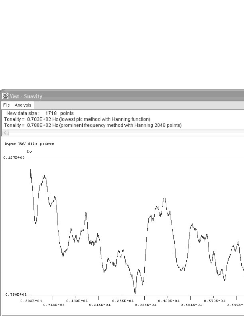
Figure 10: One cycle extracted from the signal (2 cranckshaft rotations)

Pulse analysis performed on one cycle (one period of the signal, 2 crankshaft rotations) leads to pulses marked by vertical lines in figure Fig. 11.

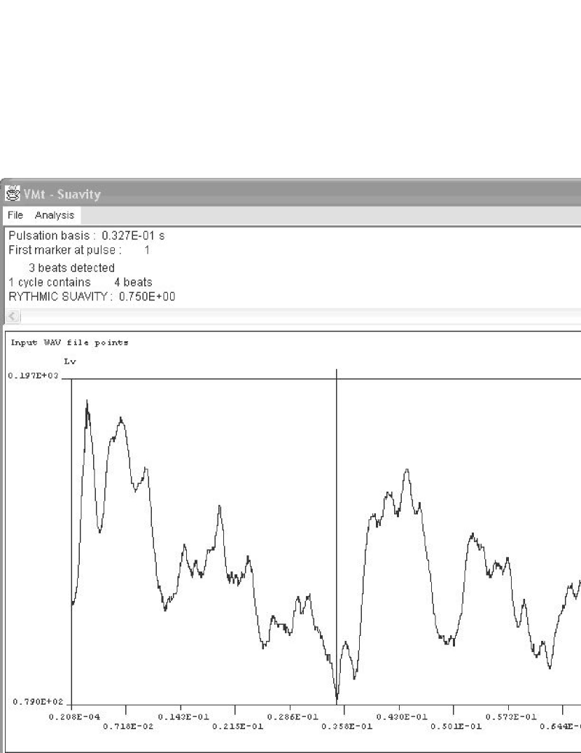
Figure 11: Detected pulses

It is found that 3 acoustic events occur at points 1, 420 and 862 during a cycle containing a total of 1718 points. Algorithmic details are illustrated in figure Fig.2. It corresponds to acoustic events occurring at pulses 0, 1 and 2 during a cycle containing 4 pulses. The rhythmic suavity of the signal is equal to $3/4=0.75$.

The periodicity of explosions suggests that the arrhythmia of the signal should be greater. Due to only 2 explosions in one period (2 explosions separated by half a rotation of the crankshaft, then no explosion during 1.5 rotation), we thought that the rhythmic suavity would be equal to $2/4=0.5$ (2 acoustic events for a total of 4 pulses).

But from figure Fig. 10, signal analysis clearly shows 3 areas: 1) a first area containing 3 decreasing peaks; 2) an ascent followed by 3 decreasing peaks; 3) a last ascent followed by several peaks without special emergence. Thus having found 3 acoustic events is correct. In fact, mechanical noises are emitted at 1/4 of the second crankshaft rotation without any explosion. The level of this third pulse is anyway less than the one of the 2 previous pulses, but its emergence is clearly present in the signal.

The analysis of durations between acoustic events agrees with the fact that a cycle is made of 4 pulses. The calculated rhythmic suavity (equal to $3/4$) is the correct one.

Tonal centre is chosen as the fundamental frequency $f_{0}=70.3$ Hz.

Table 4: Chord 1

frequencies (Hz)	$k_{n}$	$i_{n}$	Euler	Proposed
			table 1	table 3
$f_{1}=187.5$	1	5	$2^{3}3^{-1}$	$2^{-7}7^{3}$
$f_{2}=562.5$	3	0	$2^{3}$	$2^{3}$
$f_{3}=937.5$	3	9	$2^{3}3^{-1}5^{1}$	$2^{-6}3^{1}17^{2}$
$f_{4}=1406.25$	4	4	$2^{2}5^{1}$	$2^{-2}3^{1}5^{1}$
$f_{5}=1593.75$	4	6	$2^{-1}3^{2}5^{1}$	$2^{-6}31^{1}47^{1}$
$f_{6}=1875.0$	4	9	$2^{4}3^{-1}5^{1}$	$2^{-5}3^{1}17^{2}$
$f_{7}=2250.0$	5	0	$2^{5}$	$2^{5}$
$f_{8}=2718.75$	5	3	$2^{6}3^{1}5^{-1}$	$2^{1}19^{1}$
$f_{9}=3000.0$	5	5	$2^{7}3^{-1}$	$2^{-3}7^{3}$
$f_{10}=3468.75$	5	7	$2^{4}3^{1}$	$3^{2}5^{1}$
easiness			25	169
coefficient			30	128
suavity			41.46%	49.24%

Table 4 shows the frequency content of chord 1 (first column), $k_{n}$ and $i_{n}$ factors corresponding to stage 3 algorithm, and the prime decomposition according to Euler and proposed methods. Doing the same computation for the second chord yields a coefficient in Euler’s method equals to 120 to obtain only integers. For the third chord, this coefficient in Euler’s method remains equal to 120. In order to calculate the tonal suavity of the whole cycle, we have to consider only one value of this coefficient (which correspond to a shift of the tonal centre), which is obviously the greater value (in order to have only integers). Updating this coefficient to 120 in the calculation of the first chord leads to a tonal suavity of chord 1 equal to 36.58%. This updated value will be used in the computation of the averall tonal suavity.

Finally, tonal suavity (for the signal, i.e. for all chords) based on the proposed prime decomposition is equal to 36.02% and to 34.10% based on Euler’s decomposition.

The signal is composed of 3 chords. Frequencies of first chord have been presented in table 4. Frequency contents of chords 2 and 3 are given in table 5.

Table 5: Frequency content of chords 2 and 3 (Hz)

Chord 2	Chord 3
$f_{1}=281.25$	$f_{1}=140.625$
$f_{2}=937.5$	$f_{2}=234.375$
$f_{3}=1687.5$	$f_{3}=468.75$
$f_{4}=2343.75$	$f_{4}=562.5$
$f_{5}=3093.75$	$f_{5}=890.625$
$f_{6}=3656.25$	$f_{6}=1171.875$
$f_{7}=4406.25$	$f_{7}=1546.875$
$f_{8}=5062.5$	$f_{8}=1828.125$
$f_{9}=5812.5$	$f_{9}=1921.825$
$f_{10}=6468.75$	$f_{10}=2203.125$

Table 6: Chords in compact form in $\mathbb{Z}/12\mathbb{Z}$

Chord1	Chord 2	Chord 3
0	0	0
1	1	1
3	2	6
4	4	8
7	6	9
10	7
11	8
	9

From chords written in $\mathbb{Z}/12\mathbb{Z}$ in compact form, as given in table 6, it appears that there is no transformation from chord 1 to chord 2, nor from chord 3 to chord 1 (periodic signal), and chord 3 = Id(chord 2) -{2, 4, 7}.

In this case, analysis of chords transitions leads to:

• chord 1 to chord 2: harmonic suavity = tonal suavity of chord 2 with respect to the bass of chord 1 (i.e. replacing $f_{0}$ by 187.5);

• chord 2 to chord 3: harmonic suavity = 1 (transformation mark corresponding to $Id=R_{0}$);

• chord 3 to chord 1: harmonic suavity = tonal suavity of chord $\mathscr{R}_{\text{chord 3}}=\text{chord 1}$ with respect to the bass of chord 3 (i.e. replacing $f_{0}$ by 140.625).

It is important not to forget, as aforementionned, that $o_{n}=0$ when calculating harmonic suavity using tonal suavity.

Harmonic suavity of the signal is equal to 69.92% with Euler’s decomposition, and to 89.43% with the proposed one.

Finally, the noise emitted by this asymmetrical two-stroke engine as a rhythmic suavity equals to 75%, a tonal suavity equals to 36.02% and an harmonic suavity equals to 89.43%. Global suavity is equals to 42.10%.

VII.2 Symmetrical two-stroke engine

In this second example, the signal is the noise emitted by a symmetrical two-stroke engine. One explosion happens at each crankshaft rotation.

The analysis of cycles yields a mean duration equal to 0.0551 s with a standard deviation of $1.10.10^{-3}$ s. One cycle (which means 1 period, and also 1 crankshaft rotation this time) corresponds to an engine rotation speed equals to 1089 rpm.

Pulse analysis on this cycle leads to acoustic events as depicted by vertical lines in figure Fig. 12.

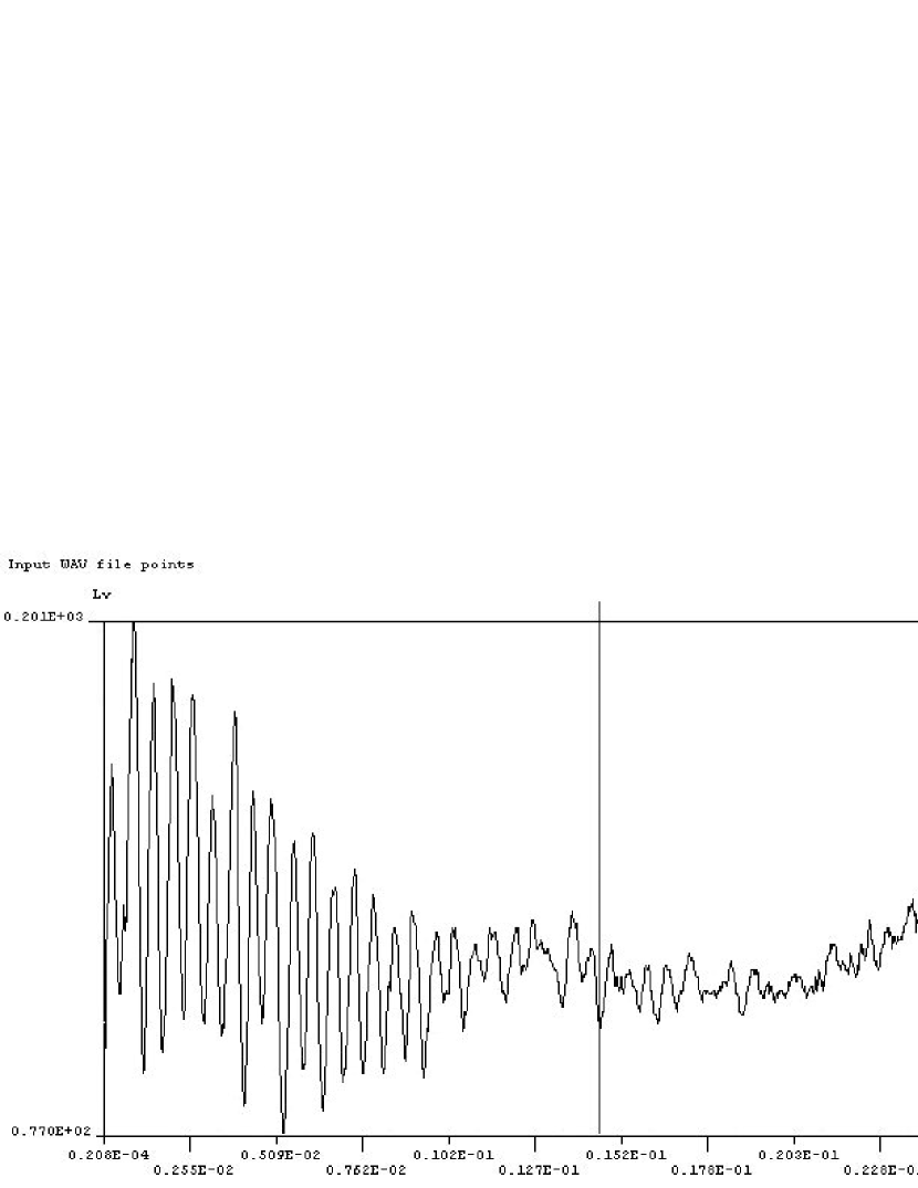
Figure 12: Detected pulses

Only 2 acoustic events are detected at points 1 and 871 in a cycle containing 2433 points. This correspond to 2 acoustic events at pulses 0 and 2 within a cycle containing a total of 5 pulses. The rhythmic suavity is equal to $2/5=0.40$.

Tonal centre is chosen as the fundamental frequency $f_{0}=11.7$ Hz, and the tonal suavity is equal to 37.85% with the proposed decomposition.

The analysis of chords transitions is reduced to transitions from chord 1 to chord 2 and from chord 2 to chord 1. In both cases, we have $\mathscr{D}=R_{10}\circ S_{0}$. Harmonic suavity is equal to 70.00% in both cases.

Finaly, global suavity is equals to 23.21%.

Comparison between asymmetrical and symmetrical two-stroke engines yields that:

• Contrary to intuition, the asymmetrical engine has a better rhythmic suavity than the symmetrical engine. This point is confirmed by a jury.

• tonal suavities are almost the same for both engines. This means that chords of both engines has the same overall beauty.

• The difference is more pronounced on the harmonic suavity. This means that the transition from a chord to the other is smoother for the asymmetrical engine.

A way to improve the noise of the symmetrical engine (compared to the asymmetrical engine) could be to add one frequency to the second acoustical event (in order to improve the harmonic suavity, but without lowering the tonal suavity), and to work on the rythmicity of the engine (for example by adding a third acoustic event).

VIII Conclusion

The purpose of the present study was to develop a tool able to give a measure of the beauty, or the acoustical quality, of (periodic) noises.

To perform this task, we decomposed this beauty into three components: rhythmic, tonal and harmonic suavity, each of them giving an indication of beauty according to a different point of view.

From an algorithmic point of view, suavity computations are performed by manipulating only array of integers, which consumes little memory and requires very low computation time.

It may be interesting to notice that harmonic suavity is a way of coding a chord from the previous one by only the dihedral and the non congruous components.

Although we have so far used a $\mathbb{Z}/12\mathbb{Z}$ decomposition, it is quite possible to use any other decomposition the moment an easyness was formalized (i.e. as in tables 1 and 3): for example the thaï-khmer musical scale uses $\mathbb{Z}/7\mathbb{Z}$, and the slendro scale used in Java uses $\mathbb{Z}/5\mathbb{Z}$bib (1971).

Finally the presented method shows excellent agreement with the feeling of a human jury (8 internal members plus customers teams) on all industrial cases treated untill now.

References

- Green (1971) D. Green, Psychological Review 78(6), 540 (1971).
- Roads (1991) C. Roads, in Computer Music Journal, edited by G. D. P. A. Piccialli and C. R. editors (The MIT Press, Cambridge, Massachusets, 1991).
- bib (006 ) Audacity 1.2.6 (audacity.sourceforge.net, Internet, 2006-).
- Lithaud et al. (008 ) A. Lithaud, N. Bogaards, and A. Roebel, AudioSculpt 2.9, edited by Ircam (Internet, 2008-).
- bib (2002) E DIN 45681 (2002).
- bib (1995) ANSI S1.13 (1995).
- Euler (1739) L. Euler, Tentamen novæ theoriæ musicæ ex certissismis harmoniæ principiis dilucide expositae [E033]. (Saint Petersburg Academy, 1739).
- Euler (1766) L. Euler, Mémoires de l’académie des sciences de Berlin 20, 165 (1766).
- Euler (1773) L. Euler, Novi Commentarii academiæ scientiarum Petropolitanæ 18, 330 (1773).
- Euler (1772) L. Euler, Lettres à un princesse d’Allemagne sur divers sujets de physique & de philosophie [E343,344,417], edited by S. P. . I. de l’Academie impériale des sciences (1768-1772).
- von Helmholtz (1877) H. L. F. von Helmholtz, On the sensations of Tone as a Physiological Basis for the Theory of Music, edited by f. G. t. E. 2nd. Ed. translation A.J. Ellis (1885) (Dover (1954), New York, 1877).
- Burley (1998) J. C. Burley, GNU Fortran g77 (GNU Project, Internet, 1998).
- bib (2003) java application programming interface (Koblenz University, Internet, 2000-2003).
- bib (1971) Encyclopædia universalis (1971).