Emerging Potentials in Higher-Derivative Gauged Chiral Models Coupled to ${\cal{N}}=1$ Supergravity

Abstract

We present a new method to introduce scalar potentials to gauge-invariant chiral models coupled to supergravity. The theories under consideration contain consistent higher-derivative terms which do not give rise to instabilities and ghost states. The chiral auxiliaries are not propagating and can be integrated out. Their elimination gives rise to emerging potentials even when there is not a superpotential to start with. We present the case of a single chiral multiplet with and without a superpotential and, in the gauged theory, up to two chiral multiplets coupled to supergravity with no superpotential. A general feature of the emergent potential is that it is negative defined leading to anti-de Sitter vacua. In the gauge models, competing D-terms may lift the potential leading to stable and metastable de Sitter and Minkowski vacua as well with spontaneously broken supersymmetry.

1 Introduction and Conclusions

Higher derivative theories are usually ill-defined in the sense that they suffer from Ostrogradski instabilities ostro . These are instabilities caused by terms linear in momentum in the Hamiltonian as a result of the higher time derivatives. Quantum mechanically these instabilities are usually shown up as ghost states. It is important therefore to determine what kind of higher-derivative interactions may give rise to consistent theories. In the case of scalars coupled to gravity for example, the consistent higher derivative theories we know, (which are also quadratic in the scalars) contain the terms

$${\cal{L}}_{I\phantom{I}} = \phi^{2}R_{GB}^{2}\,,$$ (1)

$${\cal{L}}_{II} = G^{\mu\nu}\partial_{\mu}\phi\partial_{\nu}\phi\,,$$ (2)

where

$$G_{\mu\nu}=R_{\mu\nu}-\frac{1}{2}g_{\mu\nu}R\,,~{}~{}~{}R_{GB}^{2}=R_{\mu\nu\gamma\delta}R^{\mu\nu\gamma\delta}-4R_{\mu\nu}R^{\mu\nu}+R^{2}$$ (3)

are the Einstein and the Gauss-Bonnet tensors, respectively. When more fields are involved, the general case has been discussed in hord , whereas such theories are nowadays known as galileon gal2 ; gal3 , or k-essence, for example dm ; m2 ; m1 .

That ${\cal{L}}_{I\phantom{I}}$ leads to second order evolution equation follows easily from the fact that the Gauss-Bonnet combination is a total derivative in four-dimensions and it is linear in second order derivatives. Instead, ${\cal{L}}_{II}$ leads to second order equations as, in Hamiltonian ADM formalism adm , $G_{tt}$ and $G_{it}$ contain only first time derivatives, as $G_{tt}$ and $G_{ti}$ are the Hamiltonian and momentum constraints.

In a supergravity setup now, the supersymmetrization of ${\cal L}_{I}$ has been worked out in fer1 ; fer2 and of ${\cal L}_{II}$ in ger-far . Here, we construct higher-derivative theories of k-essence type, i.e. theories that the scalar kinetic term $K(X)$ is in general a function of $X=(\partial\phi)^{2}$ dm ; m2 ; m1 . Such theories apart from their obvious interest as the most generic supersymmetric theories avoiding Ostrogradski (higher derivatives) instabilities, may also have phenomenological interest.

It should be stressed that in general there are two different types of higher derivative interactions: those which lead to equations of motions with higher than two time derivatives and those which contains at most two time derivatives. The first class leads at the classical level to the Ostrogradski instability and at the quantum level to ghost states. Here we are interested only in the second class of models where there are no higher that two time derivatives in the field equations. We also note that the higher derivative terms we are employing here are not new (they have appeared at different occasions for different reasons). Such terms have been considered before in global supersymmetry in gates ; ovrut1 ; Khoury:2010gb , in which cases the building block for the theory we consider was introduced. In particular, such term has been employed in a generic contruction of ${\cal{N}}=1$ globally supersymmetric Gallileon ovrut1 and k-essence type lagrangians Khoury:2010gb . Motivated by the latter constructions, and our earlier work in the new minimal supergravity framework ger-far , one is tempted to consider such higher derivative interactions in a locally supersymmetric setup. Although we do not have a recipe of which higher derivative interactions do not lead to higher time derivatives, the particular form of the higher derivative terms we will employ satisfy this criterion and therefore are free from Ostrogradski instabilities and ghost states. Just before the appearence of this work, another article with the same higher derivative interactions appeared in LO discussing however, the ungauged case with a single chiral multiplet.

In our work, we are focusing on the emergence of the scalar potential for more than one (two) chiral multiplets in general gauged supergravity models. A generic feature of these models is the modification of the scalar potential. The fact that higher derivative models indeed modify the effective scalar potential is known. For example, Cecotti:1986jy dicuss the structure of the scalar potential in general higher derivative theories. In this work, we construct models which explicitly realise this idea.

There are various reasons for which one should consider the most general type of potential in supersymmetric theories. At a more theoretical level, one fundamental question is if the structure of the standard scalar potential at the two derivative level is maintained when higher derivatives are included. We find, consistently with previous suggestions Cecotti:1986jy , that the scalar potential has completely different structure in the presence of higher derivatives. This has profound effects to the structure of the vacuum and the supersymmetry breaking. Also, the gauge models we are discussing (and which have not been employed previously) could lead to different Higgs sectors and potential as the two chiral multiplets we are considering could be the Higgs mutiplets. In addition, as the theory we will describe does not contain extra states besides the usual graviton and the scalars (in the bosonic sector), it can be considered as inflaton (or curvatons) in cosmology. In this context, density perturbations of the scalar fields will then be a issue to be explored. Moreover, this new scalar potential seems to have very interesting properties from the supersymmetry breaking point of view, since it breaks it spontaneously. Thus it can provide new possibilities in a hidden sector supersymmetry breaking setup.

We will consider chiral multiplets coupled to supergravity. We will write down supersymmetric actions in ${\cal{N}}=1$ superspace and explicitly work out the case of a single chiral multiplet without superpotential. We will see that in this case, the action contains quartic powers of the auxiliaries which, nevertheless, can still be eliminated by their (algebraic) equations of motions. As a result of the elimination of the chiral auxiliaries, a potential for the scalar emerges even though there is no superpotential to start with. Interesting enough, supersymmetry is always spontaneously broken and there is no supersymmetric vacuum. The same can be done when the chiral multiplet possess a superpotential as well. In this case, although more involved, the auxiliaries can still be eliminated giving rise to a quite complicated scalar potential, completely changing the standard ${\cal{N}}=1$ one. I addition, we exploit the case of more than one chiral multiplets coupled to supergravity. Although in this case, the problem is technically more difficult as one has to solve algebraic equations of increasing higher order as we increase the number of chirals , we do explicitly a two-chiral multiplets model with no superpotential.

We consider gauge invariant chiral models as well, where some of the isometries of the scalar manifold are gauged. In particular we discuss a single chiral multiplet charged under some Abelian gauge group and no superpotential. In this case, on top of the D-term contribution to the scalar potential, there exists a new contribution coming from the emergent potential after integrating out the scalar auxiliaries. We also introduce FI-terms and we find the saddle points of the potential, which may possess de Sitter, Minkowski or anti-de Sitter symmetry. Again supersymmetry is always spontaneously broken and there is no supersymmetric vacuum. Finally, we also discuss gauge models with two chiral charged multiplets and no-superpotential. This case can also be solved exactly with similar results.

The lesson from these considerations is that higher derivative terms in supergravity contribute also to the potential terms. Thus, theories with no potential at the leading two-derivative level, may develop nontrivial potential when higher derivatives are taken into account. At this point there are however, two dangerous aspects. The first one concerns the appearance of the Ostrogradski instability. In the type of theories we are discussing, this instability is not present as the theory although with higher derivatives, gives rise to equations of motion with maximum second order time derivatives. This guarantees causal propagation and no-unphysical ghost states. The second issue concerns the auxiliary fields. Here, we were able still to eliminate the auxiliaries of the chiral multiplet since they appeared algebraically in the supersymmetric Lagrangian. In fact, only the modulus of the auxiliary could be eliminated while its phase is propagating. This is enough however, as in the bosonic action, only its modulus appear and therefore can be integrated out. It may happen, and this is the rule actually, that in supersymmetric theories with higher-derivatives, the auxiliaries turns out to be dynamical and propagating. In that case, they can not be eliminated and they should be kept in the total Lagrangian. Under such circumstances there is no emergent potential.

Summarizing, we stress that the standard form of the supersymmetric potential for chiral fields coupled to ${\cal{N}}=1$ supergravity

$$V=e^{K}\left[g^{i{\bar{j}}}(D_{i}P)(D_{\bar{j}}\bar{P})-3P\bar{P}\right]$$ (4)

is only valid at the leading two-derivative level. Introduction of appropriate higher derivative terms that do not give rise to pathologies and inconsistencies, modifies considerably the structure of (4) and give rise to a kind of emergent potential even in cases where there is no one to start with (i.e. no superpotential). In this case, supersymmetry is always spontaneous broken with de Sitter, Minkowski or anti-de Sitter maximally symmetric vacua. This is also true in the case of gauged models with or without FI-terms.

In the next section 2. we present the higher-derivative chiral model coupled to ${\cal{N}}=1$ supergravity. In section 3. we discuss the emergent potential of a single chiral multiplet with and without superpotential and in section 4. we present the emergent potentials for gauge models.

2 Chiral Models with Higher Derivatives in Supergravity

Let us consider the most general (two-derivative) superspace Lagrangian of chiral superfields coupled to supergravity in superspace formalism

$${\cal{L}}_{0}=\frac{1}{\kappa^{2}}\int d^{2}\Theta\,\,2{\cal{E}}\left[\frac{3}{8}\Big{(}\bar{{\cal{D}}}\bar{{\cal{D}}}-8{\cal{R}}\Big{)}\,e^{-\frac{\kappa^{2}}{3}K(\Phi^{i},\bar{\Phi}^{\bar{j}})}+\kappa^{2}P(\Phi)\right]+h.c.$$ (5)

The hermitian function $K(\Phi^{i},\bar{\Phi}^{\bar{j}})$ is the Kähler potential Zumino:1979et , $P(\Phi^{i})$ is the superpotential (a holomorphic function of the chiral superfields $\Phi^{i}$) and $\kappa$ is proportional to the Planck length, which from now on will be set equal to 1. The abbreviations

$$\bar{{\cal{D}}}_{\dot{\alpha}}\bar{{\cal{D}}}^{\dot{\alpha}}=\bar{{\cal{D}}}\bar{{\cal{D}}}\,,~{}~{}~{}~{}~{}{\cal{D}}^{\alpha}{\cal{D}}_{\alpha}={\cal{D}}{\cal{D}}$$ (6)

will be used for the sum of the fermionic superspace covariant derivatives and $\int d^{2}\Theta$ is the super-integration over the so called new $\Theta$ variables. From the supergravity multiplet sector, $2{\cal{E}}$ is the usual chiral density employed to create supersymmetric Lagrangians, which in the new $\Theta$ variables has the expansion

$$2{\cal{E}}=e\left\{1+i\Theta\sigma^{a}\bar{\psi}_{a}-\Theta\Theta\Big{(}M^{*}+\bar{\psi}_{a}\bar{\sigma}^{ab}\bar{\psi}_{b}\Big{)}\right\}$$ (7)

in terms of the vielbein ($e_{m}^{a}$), the gravitino ($\psi_{m}$) and the complex scalar auxiliary field $M$. We also mention that the off-shell minimal supergravity multiplet also contains another auxiliary field, the real vector $b_{a}$. In addition, ${\cal{R}}$, the superspace curvature, is a chiral superfield which contains the Ricci scalar in its highest component. In the matter sector, $\Phi^{i}$ and $\bar{\Phi}^{\bar{j}}$ denote a set on chiral and anti-chiral superfields ($\bar{{\cal{D}}}_{\dot{\alpha}}\Phi^{i}=0$, ${\cal{D}}_{\alpha}\bar{\Phi}^{\bar{j}}=0$) whose components are defined via projection

$$A^{i} = \Phi^{i}|_{\theta=\bar{\theta}=0},$$

$$\chi^{i}_{\alpha} = \frac{1}{\sqrt{2}}{\cal{D}}_{\alpha}\Phi^{i}|_{\theta=\bar{\theta}=0},$$ (8)

$$F^{i} = -\frac{1}{4}{\cal{D}}{\cal{D}}\Phi^{i}|_{\theta=\bar{\theta}=0}.$$

After calculating the component form of (5), integrating out the auxiliary fields and performing a Weyl rescaling of the gravitational field (accompanied by a redefinition of the fermionic fields), the pure bosonic Lagrangian reads

$$e^{-1}{\cal{L}}_{0}=-\frac{1}{2}R-g_{i{\bar{j}}}\partial_{a}A^{i}\partial^{a}\bar{A}^{\bar{j}}-\ e^{K}\left[g^{i{\bar{j}}}(D_{i}P)(D_{\bar{j}}\bar{P})-3P\bar{P}\right].$$ (9)

Further details maybe found for example in Wess:1992cp . Here

$$g_{i{\bar{j}}}=\frac{\partial^{2}K(A,\bar{A})}{\partial A^{i}\partial\bar{A}^{\bar{r}}}$$ (10)

is the positive definite Kähler metric, on the manifold parametrized by $A^{i}$ and $\bar{A}^{\bar{j}}$. Moreover, the Kähler space covariant derivatives are defined as follows

$$D_{i}P=P_{i}+K_{i}P$$ (11)

where

$$P_{i}=\frac{\partial P}{\partial A^{i}}\,,~{}~{}~{}~{}K_{i}=\frac{\partial K}{\partial A^{i}}\,.$$ (12)

The Lagrangian (9) is Kähler invariant as long as the superpotential scales as

$$P(A^{i})\rightarrow e^{-S(A^{i})}P(A^{i})$$ (13)

under a Kähler transformation

$$K(A^{i},\bar{A}^{\bar{j}})\rightarrow K(A^{i},\bar{A}^{\bar{j}})+S(A^{i})+\bar{S}(\bar{A}^{\bar{j}}),$$ (14)

where $S(A^{i})$ and $\bar{S}(\bar{A}^{\bar{j}})$ are holomorphic functions of the complex coordinates. From the form of the supersymmetry transformations of the fermions one can see that

$$\delta_{susy}\chi\sim F$$ (15)

Thus, supersymmetry is broken whenever

$$<D_{i}P>\neq 0$$ (16)

since on-shell

$$F^{*}\sim-\frac{\partial P}{\partial A}-P\frac{\partial K}{\partial A}=D_{A}P\,.$$ (17)

This fact leads to the conclusion that it is possible to have supersymmetric anti-de Sitter (AdS) or Minkowski vacua but not de Sitter (dS) ones since $-3P\bar{P}\leq 0$ always. It should be stressed that this is a property of the superpotential and not a general property of the supergravity theory after integrating out the auxiliary sector. Indeed, there are cases where anti-de Sitter vaccua maybe uplifted to de Sitter ones Kachru:2003aw ; Villadoro:2005yq ; Catino:2011mu .

2.1 Higher Derivative Chiral Models

Higher derivative couplings have extensively been studied. Nevertheless, not all possible such higher derivative terms have an exact supergravity counterpart, and some might not have one at all. The theory we are interested in, has a superspace Lagrangian of the form

$${\cal{L}}={\cal{L}}_{0}+{\cal{L}}_{HD}$$ (18)

where ${\cal{L}}_{0}$ is the standard superspace supergravity Lagrangian given in eq.(5) and

$${\cal{L}}_{HD}=\int d^{2}\Theta\,\,2{\cal{E}}\left\{\frac{1}{8}\Big{(}\bar{{\cal{D}}}\bar{{\cal{D}}}-8{\cal{R}}\Big{)}\Lambda^{\bar{r}i\bar{n}j}\Big{[}\bar{{\cal{D}}}_{\dot{\alpha}}K_{i}{\cal{D}}_{\alpha}K_{\bar{r}}\bar{{\cal{D}}}^{\dot{\alpha}}K_{j}{\cal{D}}^{\alpha}K_{\bar{n}}\Big{]}\right\}+h.c.$$ (19)

Note that (19) appeared first in LO just before present work released wheras the flat-space limit of (19) with global supersymmetry appeared in gates ; Khoury:2010gb . It is important that ${\cal{L}}$ is manifestly both Kähler and (independently) super-Weyl invariant, as will be seen later on. These two symmetry properties, although obviously they do not specify the form of the action, they are essential in the consistency of the model as well as for the supergravity theory that it describes. As we will see, (19) does not involve derivatives of the auxiliary fields, which are not propagating and can be integrated out. Equivalently, (19) can be expressed in terms of the chiral superfields $\Phi^{i}$ as

$${\cal{L}}_{HD}=\int d^{2}\Theta\,\,2{\cal{E}}\left\{\frac{1}{8}\Big{(}\bar{{\cal{D}}}\bar{{\cal{D}}}-8{\cal{R}}\Big{)}\Lambda_{i\bar{r}j\bar{n}}\Big{[}\bar{{\cal{D}}}_{\dot{\alpha}}{\bar{\Phi}}^{\bar{r}}{\cal{D}}_{\alpha}\Phi^{i}\bar{{\cal{D}}}^{\dot{\alpha}}{\bar{\Phi}}^{\bar{n}}{\cal{D}}^{\alpha}\Phi^{j}\Big{]}\right\}+h.c.$$ (20)

where

$$K_{i\bar{r}}=\frac{\partial^{2}K(\Phi,\bar{\Phi})}{\partial\Phi^{i}\partial\bar{\Phi}^{\bar{r}}}$$ (21)

is the Kähler metric on the complex space spanned by the chiral and anti-chiral superfields and $\Lambda_{i\bar{r}j\bar{n}}$ represents a Kähler tensor. For example, one may choose

$${\Lambda}_{i\bar{r}j\bar{n}}={\cal{G}}(\Phi,\bar{\Phi})K_{i\bar{r}}K_{j\bar{n}}+{\cal{H}}(\Phi,\bar{\Phi}){\cal{R}}_{i\bar{r}j\bar{n}}$$ (22)

with ${\cal{G}}(\Phi,\bar{\Phi})$ and ${\cal{H}}(\Phi,\bar{\Phi})$ being some Kähler invariant hermitian functions and ${\cal{R}}_{i\bar{r}j\bar{n}}$ the Kähler space Riemann tensor defined as

$${\cal{R}}_{i\bar{j}k\bar{l}}=\frac{\partial}{\partial{\Phi}^{i}}\frac{\partial}{\partial{\bar{\Phi}}^{\bar{j}}}K_{k\bar{l}}-K^{m\bar{n}}\left(\frac{\partial}{\partial{\bar{\Phi}}^{\bar{j}}}K_{m\bar{l}}\right)\left(\frac{\partial}{\partial{\Phi}^{i}}K_{k\bar{n}}\right).$$ (23)

The form (22) implies some symmetries for the Kähler indices which, without loss of further generality, we will assume to be possessed by all the $\Lambda_{i\bar{r}j\bar{n}}$ to be considered in this work. Our next task is to extract the component field expression for the Lagrangian (20), which after superspace integration turns out to be

$$e^{-1}{\cal{L}}_{HD}=-16\ {\cal{U}}_{i\bar{r}j\bar{n}}\!\! \!\!\Big{(}F^{i}F^{j}\bar{F}^{\bar{r}}\bar{F}^{\bar{n}}+\partial_{a}A^{i}\partial^{a}A^{j}\partial_{b}\bar{A}^{\bar{r}}\partial^{b}\bar{A}^{\bar{n}}$$ (24)

$$-F^{i}\bar{F}^{\bar{r}}\partial_{a}A^{j}\partial^{a}\bar{A}^{\bar{n}}-F^{i}\bar{F}^{\bar{n}}\partial_{a}A^{j}\partial^{a}\bar{A}^{\bar{r}}\Big{)}.$$

for the pure bosonic sector. In (24) we have used the notation

$${\cal{U}}_{i\bar{r}j\bar{n}}(A,\bar{A})=\Lambda_{i\bar{r}j\bar{n}}(\Phi,\bar{\Phi})\Big{|}_{\theta=\bar{\theta}=0}$$ (25)

Again it is easy to see that (24) is manifestly Kähler invariant.

2.2 Super-Weyl Invariance

At this point its is crucial to make a comment on a subtlety concerning the hermitian vector superfield

$$V=\Lambda_{i\bar{r}j\bar{n}}\bar{{\cal{D}}}_{\dot{\alpha}}{\bar{\Phi}}^{\bar{r}}{\cal{D}}_{\alpha}\Phi^{i}\bar{{\cal{D}}}^{\dot{\alpha}}{\bar{\Phi}}^{\bar{n}}{\cal{D}}^{\alpha}\Phi^{j},$$ (26)

namely, its scaling properties under super-Weyl transformations. We emphasize that $V$ is defined through its components. For example, its lowest component will be

$$V\Big{|}_{\theta=\bar{\theta}=0} = 4\ {\cal{U}}_{i\bar{r}j\bar{n}}\ \bar{\chi}_{\dot{\alpha}}^{\bar{r}}\chi_{\alpha}^{i}\bar{\chi}^{\dot{\alpha}\bar{n}}\chi^{{\alpha}j}.$$ (27)

Moreover, all components of $V$ should be understood as those of a hermitian vector superfield defined via projection and will eventually be related to (2). This definition will gives Weyl weight $-2$ to the vector superfield $V$, as is required so that (20) is indeed Kähler and super-Weyl invariant. These symmetries are crucial for consistency of the supergravity Lagrangian on curved superspace. Under a super-Weyl transformation, the superspace covariant derivatives change as Dragon:1986ew

$$\delta_{\Sigma}{\cal{D}}_{\alpha}=(\Sigma-2\bar{\Sigma}){\cal{D}}_{\alpha}-({\cal{D}}^{\gamma}\Sigma)l_{\alpha\gamma}$$

$$\delta_{\Sigma}\bar{\cal{D}}_{\dot{\alpha}}=(\bar{\Sigma}-2\Sigma)\bar{\cal{D}}_{\dot{\alpha}}-(\bar{\cal{D}}^{\dot{\gamma}}\bar{\Sigma})l_{\dot{\alpha}\dot{\gamma}}$$ (28)

where the $l_{\alpha\gamma}$ and $l_{\dot{\alpha}\dot{\gamma}}$ stand for the (anti)self-dual parts of infinitesimal Lorentz transformations. Moreover, by choosing $\Phi^{i}$ and the tensor $\Lambda_{i\bar{r}j\bar{n}}$ to have vanishing Weyl weights, i.e.

$$\delta_{\Sigma}{\Lambda}_{i\bar{r}j\bar{n}}=\delta_{\Sigma}{\Phi}^{i}=\delta_{\Sigma}\bar{\Phi}^{\bar{r}}=0,$$ (29)

and by using (2.2), one may straightforwardly check that under a super-Weyl transformation, the vector superfield (26), scales as

$$\delta_{\Sigma}(\Lambda_{i\bar{r}j\bar{n}}\bar{{\cal{D}}}_{\dot{\alpha}}{\bar{\Phi}}^{\bar{r}}{\cal{D}}_{\alpha}\Phi^{i}\bar{{\cal{D}}}^{\dot{\alpha}}{\bar{\Phi}}^{\bar{n}}{\cal{D}}^{\alpha}\Phi^{j})=-2(\Sigma+\bar{\Sigma})(\Lambda_{i\bar{r}j\bar{n}}\bar{{\cal{D}}}_{\dot{\alpha}}{\bar{\Phi}}^{\bar{r}}{\cal{D}}_{\alpha}\Phi^{i}\bar{{\cal{D}}}^{\dot{\alpha}}{\bar{\Phi}}^{\bar{n}}{\cal{D}}^{\alpha}\Phi^{j}).$$ (30)

Of course, when we perform the super-Weyl rescaling to our Lagrangian (20), we have to consider the variation of the involved superfields in the new $\Theta$ variables Wess:1992cp .

3 The Emergent Potential

The main result in this section is to show that, even in those theories where there is no superpotential, a scalar potential can still be introduced through higher derivatives. A hint that this is indeed the case, emerges from the fact that higher derivative matter couplings are likely to change the scalar potential as soon as the equations of motion for the auxiliary fields are solved and plugged-back into the action Cecotti:1985mf ; Cecotti:1987sa ; fer2 ; Cecotti:1986jy ; Cecotti:1986pk ; Krasnikov:1989ry ; Sasaki:2012ka ; Khoury:2010gb .

3.1 A Single Chiral Multiplet with no Superpotential

In order to illustrate the appearance of a scalar potential when the superpotential is vanishing, we need to make the effect of the new coupling (19) more transparent. Towards this target, we will consider first a theory with only one chiral multiplet and no superpotential. We will discuss this case first as it will better illustrate our results. In addition, absence of a superpotential may be forced by global symmetries (R-symmetry for example) which might forbid its appearance. In this case, the Lagrangian (18) is explicitly written as

$${\cal{L}}=\int d^{2}\Theta\,\,2{\cal{E}}\left\{\Big{(}\bar{{\cal{D}}}\bar{{\cal{D}}}-8{\cal{R}}\Big{)}\left[\frac{3}{8}e^{-\frac{1}{3}K}+\frac{1}{8}\Lambda\ \bar{{\cal{D}}}_{\dot{\alpha}}{\bar{\Phi}}{\cal{D}}_{\alpha}\Phi\bar{{\cal{D}}}^{\dot{\alpha}}{\bar{\Phi}}{\cal{D}}^{\alpha}\Phi\right]\right\}+h.c.$$ (31)

with $\Lambda$ being an abbreviation for ${\Lambda}_{{\Phi}\bar{{\Phi}}{\Phi}\bar{{\Phi}}}$, a hermitian and Kähler invariant function of $\Phi$ and $\bar{\Phi}$. In component form, the bosonic sector of the Lagrangian (31) turns out to be (after integrating out the auxiliary fields $M$ and $b_{a}$, and subsequent appropriately rescalings)

$$e^{-1}{\cal{L}}_{\rm{bos}} = -\frac{1}{2}R-g_{A{\bar{A}}}\partial_{a}A\partial^{a}\bar{A}+g_{A{\bar{A}}}\ e^{\frac{K}{3}}F\bar{F}$$ (32)

$$-16\ {\cal{U}}\ \left\{\phantom{\frac{X^{X}}{X^{X}}}\!\!\!\!\!\!\!\!\!\!\!e^{\frac{2K}{3}}(F\bar{F})^{2}+\partial_{a}A\partial^{a}A\partial_{b}\bar{A}\partial^{b}\bar{A}-2e^{\frac{K}{3}}F\bar{F}\partial_{a}A\partial^{a}\bar{A}\,\right\}$$

where ${\cal{U}}$ is a hermitian Kähler invariant function of the scalar field (it is the lowest component of $\Lambda$, eq.(25)). The equation of motion for $F$ is

$$\bar{F}\Big{(}g_{A{\bar{A}}}-32\ {\cal{U}}e^{\frac{K}{3}}F\bar{F}+32\ {\cal{U}}\partial_{a}A\partial^{a}\bar{A}\Big{)}=0$$ (33)

which can be easily solved for

$$F\bar{F}=e^{\frac{-K}{3}}\left(\frac{g_{A\bar{A}}}{32\ {\cal{U}}}+\partial_{a}A\partial^{a}\bar{A}\right).$$ (34)

The other solution $F=0$ brings us back to the standard supergravity case. Two important comments are in order here. First, one can see that the condition of supersymmetry breaking is changed. The vev of $F$, which is related to $\delta_{susy}\chi$, is no longer connected to the derivative of the superpotential. It is rather proportional to the potential itself, a fact that is reminiscent of the D-term supersymmetry breaking. This is not that surprising since (26) is a vector superfield in any case. Moreover, in the vacuum, since $F\bar{F}$ is positive, ${\cal{U}}$ has to be positive defined. The on-shell Lagrangian is then

$$e^{-1}{\cal{L}}_{\rm{bos}}=-\frac{1}{2}R+\frac{(g_{A{\bar{A}}})^{2}}{64\ {\cal{U}}}-16\ {\cal{U}}\partial_{a}A\partial^{a}A\partial_{b}\bar{A}\partial^{b}\bar{A}+16\ {\cal{U}}\partial_{a}A\partial^{a}\bar{A}\partial_{b}A\partial^{b}\bar{A}.$$ (35)

What has happened here has completely changed the dynamics of the theory. The minimal kinematic term for the scalar is lost, and we are only left with terms strongly resembling the k-essence m1 ; m2 . Much more interesting is the appearance of an emerging scalar potential

$${\cal{V}}=-\frac{1}{64}\frac{(g_{A{\bar{A}}})^{2}}{{\cal{U}}}.$$ (36)

From the positivity of  ${\cal{U}}$ we see that the potential (36) is negative defined

$${\cal{V}}<0$$ (37)

and therefore the theory may only have anti-de Sitter vacua. Another important property of the emerging potential is that it is not built from a holomorphic function.

In order an emerging potential to appear in higher derivative theories with chiral multiplets, two fundamental issues should be satisfied

1. Instabilities and ghosts states due to higher derivatives should not appear, and

2. the auxiliary $F$ should not be propagating in which case it can not be integrated out algebraically

The above issues probably make the interaction (31) unique and to our knowledge there is no other higher derivative coupling that can successfully satisfy the above criteria and give rise to an emerging potential. In the framework of new-minimal supergravity, consistent higher derivative terms which satsify the above restrictions have been considered ger-far ; Germani:2011cv , but no scalar potential emerged in that case. Higher derivative interactions have been also studied in bauman , but in that case instabilities appear (as it leads to higher order equations of motions and thus to Ostrogradski instabilities). Moreover the auxiliary sector can not be integrated out. Finally, it should be noted that there is work done in higher derivative matter couplings in the context of conformal supergravity as well, see for example deWit:2010za .

3.2 A Single Chiral Multiplet with Superpotential

Let us now consider the same single chiral theory but now with a non-trivial superpotential. In this case, the superspace Lagrangian will explicitly be written as

$${\cal{L}}_{P}=\int d^{2}\Theta\,\,2{\cal{E}}\left\{\Big{(}\bar{{\cal{D}}}\bar{{\cal{D}}}-8{\cal{R}}\Big{)}\left[\frac{3}{8}e^{-\frac{1}{3}K}+\frac{1}{8}\Lambda\ \bar{{\cal{D}}}_{\dot{\alpha}}{\bar{\Phi}}{\cal{D}}_{\alpha}\Phi\bar{{\cal{D}}}^{\dot{\alpha}}{\bar{\Phi}}{\cal{D}}^{\alpha}\Phi\right]+P(\Phi)\right\}+h.c.$$ (38)

In component form, after integrating out the auxiliary fields $M$ and $b_{a}$ and performing appropriate rescalings, the bosonic sector of the Lagrangian (38) turns out to be

$$e^{-1}{\cal{L}}_{P}^{\rm{bos}} = -\frac{1}{2}R-g_{A{\bar{A}}}\partial_{a}A\partial^{a}\bar{A}+g_{A{\bar{A}}}\ e^{\frac{K}{3}}F\bar{F}$$

$$+e^{\frac{2K}{3}}\Big{(}PFK_{A}+\bar{P}\bar{F}K_{\bar{A}}+P_{A}F+\bar{P}_{\bar{A}}\bar{F}\Big{)}+3e^{K}P\bar{P}$$

$$-16\ {\cal{U}}\ \Big{\{}e^{\frac{2K}{3}}\big{(}F\bar{F}\big{)}^{2}+\partial_{a}A\partial^{a}A\partial_{b}\bar{A}\partial^{b}\bar{A}-2e^{\frac{K}{3}}F\bar{F}\partial_{a}A\partial^{a}\bar{A}\Big{\}}.$$

In order to extract the on-shell theory we should eliminate the rest of the non-dynamical degrees of freedom, a non-trivial procedure as we shall see. The equation of motion for $F$ reads

$$\bar{F}\Big{\{}g_{A{\bar{A}}}-32\ {\cal{U}}e^{\frac{K}{3}}\big{(}F\bar{F}\big{)}+32\ {\cal{U}}\partial^{a}A\partial^{a}\bar{A}\Big{\}}=-e^{\frac{K}{3}}\Big{(}PK_{A}+P_{A}\Big{)}.$$ (40)

Let us now define

$$a =-32\ {\cal{U}}e^{\frac{K}{3}},$$

$$b =g_{A\bar{A}}+32\ {\cal{U}}\partial^{a}A\partial^{a}\bar{A},$$

$$c =e^{\frac{K}{3}}\Big{|}PK_{A}+P_{A}\Big{|},$$

$$x =F\bar{F}$$

in terms of which equation (40), after being multiplied by its hermitian conjugate, turns out to be

$$x(ax+b)^{2}=c^{2}.$$ (42)

Using Cardano’s method, the solutions for $x_{(i)}$ ($i=0,1,2$), are

$$x_{(i)} =-\frac{2b}{3a}+t_{(i)},$$ (43)

$$t_{(i)} =\omega^{i}\left(-\frac{q}{2}-\sqrt{\frac{q^{2}}{4}+\frac{p^{3}}{27}}\right)^{1/3}-\omega^{3-i}\ \frac{p}{3}\left(-\frac{q}{2}-\sqrt{\frac{q^{2}}{4}+\frac{p^{3}}{27}}\right)^{-1/3},$$

$$\omega =-\frac{1}{2}+i\frac{\sqrt{3}}{2}$$

with

$$p =-\frac{b^{2}}{3a^{2}},$$ (44)

$$q =-\frac{2b^{3}}{27a^{3}}-\frac{c^{2}}{a^{2}}.$$

Therefore, the on-shell Lagrangian in terms of the $t_{i}$, will have the form

$$e^{-1}{\cal{L}}_{P}^{\rm{bos}}|_{t_{i}}= -\frac{1}{2}R-g_{A{\bar{A}}}\partial_{a}A\partial^{a}\bar{A}-16\ {\cal{U}}\partial_{a}A\partial^{a}A\partial_{b}\bar{A}\partial^{b}\bar{A}$$ (45)

$$+3e^{K}P\bar{P}-e^{\frac{K}{3}}\left[\frac{3}{2}a(t_{i})^{2}-bt_{i}\right]$$

and supersymmetry is broken for

$$\langle x_{(i)}\rangle=\langle-\frac{2b}{3a}+t_{(i)}\rangle\neq 0.$$ (46)

These solutions correspond to three different perturbative vacua of (3.2). The standard road is to plug $x_{0}$ into the theory. This corresponds to the ordinary vacuum of minimal supergravity, as has been argued by recent work in global supersymmetry Khoury:2010gb ; Sasaki:2012ka . This can be seen first of all by the supersymmetry breaking signal, which remains $PK_{A}+P_{A}\neq 0$. A more extensive treatment on this can be found in a resent work Sasaki:2012ka in the context of supersymmetry and in LO in the context of supergravity.

4 Gauge Invariant Models

The Lagrangian (31) can be straightforwardly be generalized to include gauge invariant interactions Ferrara:1974pu ; Cremmer:1982en ; Cremmer:1982wb ; Bagger:1982ab . In this case, the gauge invariant superspace Lagrangian is

$${\cal{L}}_{tot}=\int d^{2}\Theta\,\,2{\cal{E}}\left\{\frac{3}{8}\Big{(}\bar{{\cal{D}}}\bar{{\cal{D}}}-8{\cal{R}}\Big{)}e^{-{\tilde{K}}/3}+\frac{1}{16g^{2}}H_{(ab)}(\Phi)W^{(a)}W^{(b)}+P(\Phi)\right.$$ (47)

$$\hskip 85.35826pt\left.+\frac{1}{8}\Big{(}\bar{{\cal{D}}}\bar{{\cal{D}}}-8{\cal{R}}\Big{)}\left[{\tilde{\Lambda}}^{\bar{r}i\bar{n}j}\ \bar{{\cal{D}}}_{\dot{\alpha}}{\tilde{K}}_{i}{\cal{D}}_{\alpha}{\tilde{K}}_{\bar{r}}\bar{{\cal{D}}}^{\dot{\alpha}}{\tilde{K}}_{j}{\cal{D}}^{\alpha}{\tilde{K}}_{\bar{n}}\right]\right\}+h.c.$$

where

$${\tilde{K}}=K(\Phi,\bar{\Phi})+\Gamma(\Phi,\bar{\Phi},V),$$ (48)

and

$$\Gamma(\Phi,\bar{\Phi},V)=V^{(a)}{\cal{D}}^{(a)}+\frac{1}{2}g_{i{\bar{r}}}X^{i(a)}{\bar{X}}^{\bar{r}(b)}V^{(a)}V^{(b)}.$$ (49)

In addition, as usual, $V^{(a)}$ is the supersymmetric Yang-Mills vector multiplet and

$$W_{\alpha}=W_{\alpha}^{(a)}T^{(a)}=-\frac{1}{4}\Big{(}\bar{{\cal{D}}}\bar{{\cal{D}}}-8{\cal{R}}\Big{)}e^{-V}{\cal{D}}_{\alpha}e^{V}$$ (50)

is the gauge invariant chiral superfield containing the gauge field strength. The holomorphic function $H_{(ab)}$ is included for generality, but in what follows we will consider $H_{(ab)}=\delta_{(ab)}$. Expression (49) is calculated in the Wess-Zumino gauge, ${\cal{D}}^{(a)}$ are the so-called Killing potentials whereas $X^{i(a)}$ and ${\bar{X}}^{\bar{r}(b)}$ are the components of the holomorphic Killing vectors that generate the isometries of the Kähler manifold. The Killing vectors and the Killing potential are connected via

$$g_{i{\bar{r}}}{\bar{X}}^{\bar{r}(a)}=i\frac{\partial}{\partial a^{i}}{\cal{D}}^{(a)},$$ (51)

$$g_{i{\bar{r}}}X^{i(a)}=-i\frac{\partial}{\partial{\bar{a}}^{\bar{r}}}{\cal{D}}^{(a)}$$ (52)

where $a^{i}$ and ${\bar{a}}^{\bar{r}}$ are the Kähler space complex co-ordinates. We note that the ${\cal{D}}^{(a)}$ that correspond to some $U(1)$ gauged symmetry are only determined up to a constant $\xi$, which is the analog for the Fayet-Iliopoulos D-term in supergravity. Now ${\tilde{\Lambda}}^{\bar{r}i\bar{n}j}$ has to respect all the isometries of the Kähler manifold. Again, following the standard procedure, the bosonic part of the Lagrangian (47) turns out to be

$$e^{-1}{\cal{L}}_{tot}= -\frac{1}{2}R-g_{i{\bar{r}}}{\tilde{D}}_{m}A^{i}{\tilde{D}}^{m}\bar{A}^{\bar{r}}+e^{\frac{K}{3}}g_{i{\bar{r}}}F^{i}\bar{F}^{\bar{r}}$$

$$-\frac{1}{16g^{2}}F_{mn}^{(a)}F^{mn(a)}-\frac{1}{2}g^{2}\big{(}{\cal{D}}^{(a)}\big{)}^{2}$$

$$-\ e^{\frac{2K}{3}}\Big{(}F^{i}D_{i}P+\bar{F}^{\bar{r}}D_{\bar{r}}\bar{P}\Big{)}+3e^{K}P\bar{P}$$

$$-16\ \tilde{{\cal{U}}}_{i\bar{r}j\bar{n}}\Big{(}e^{\frac{2K}{3}}F^{i}F^{j}\bar{F}^{\bar{r}}\bar{F}^{\bar{n}}+{\tilde{D}}_{a}A^{i}{\tilde{D}}^{a}A^{j}{\tilde{D}}_{b}\bar{A}^{\bar{r}}{\tilde{D}}^{b}\bar{A}^{\bar{n}}$$

$$\ \ \ \ \ \ \ \ \ \ -e^{\frac{K}{3}}F^{i}\bar{F}^{\bar{r}}{\tilde{D}}_{a}A^{j}{\tilde{D}}^{a}\bar{A}^{\bar{n}}-e^{\frac{K}{3}}F^{i}\bar{F}^{\bar{n}}{\tilde{D}}_{a}A^{j}{\tilde{D}}^{a}\bar{A}^{\bar{r}}\Big{)}.$$

We note that

$${\tilde{D}}_{c}A^{j}=\partial_{c}A^{j}-\frac{1}{2}B_{c}^{(a)}X^{j}_{(a)}$$ (54)

is the covariant derivative and $B_{c}^{(a)}$ is a vector field (belonging to the $V^{(a)}$ vector multiplet) that corresponds to the gauged isometries, with field strength $F_{mn}^{(a)}$.

4.1 Emergent Potential for a Single Chiral Multiplet with no Superpotential

In order to illustrate the properties of the emergent potential in the case of gauged models, our first example will be a single chiral multiplet with no superpotential. In this case the Lagrangian (4) is

$$e^{-1}{\cal{L}}_{tot}= -\frac{1}{2}R-g_{A{\bar{A}}}{\tilde{D}}_{m}A{\tilde{D}}^{m}\bar{A}+e^{\frac{K}{3}}g_{A{\bar{A}}}F\bar{F}$$

$$-\frac{1}{16g^{2}}F_{mn}^{(a)}F^{mn(a)}-\frac{1}{2}g^{2}\big{(}{\cal{D}}^{(a)}\big{)}^{2}$$

$$-16\ \tilde{{\cal{U}}}\Big{(}e^{\frac{2K}{3}}(F\bar{F})^{2}+{\tilde{D}}_{a}A{\tilde{D}}^{a}A{\tilde{D}}_{b}\bar{A}{\tilde{D}}^{b}\bar{A}-2\ e^{\frac{K}{3}}F\bar{F}{\tilde{D}}_{a}A{\tilde{D}}^{a}\bar{A}\Big{)}.$$

The single auxiliary field $F$ can now be eliminated from (4.1) by its equations of motion, leading to

$$F\bar{F}=e^{\frac{-K}{3}}\left(\frac{g_{A\bar{A}}}{32\ \tilde{{\cal{U}}}}+{\tilde{D}}_{a}A{\tilde{D}}^{a}\bar{A}\right).$$ (56)

Plugging (56) back in (4.1), we can easily read-off the potential for the gauged model which turns out to be

$${\cal{V}}=\frac{1}{2}g^{2}\left({\cal{D}}^{(a)}\right)^{2}-\frac{(g_{A\bar{A}})^{2}}{64\ \tilde{{\cal{U}}}}$$ (57)

with $\tilde{{\cal{U}}}=\tilde{{\cal{U}}}_{A\bar{A}A\bar{A}}$, a Kähler-space tensor that respects all the isometries of the gauged group. For a first example we will take a flat model with Kähler potential

$$K=a\bar{a}+d\,$$ (58)

which leads to

$$g_{a\bar{a}}=1\,,~{}~{}~{}~{}{\cal{R}}_{a\bar{a}a\bar{a}}=0$$ (59)

The $U(1)$ Killing potential is

$$D^{(1)}=a\bar{a}+\xi$$ (60)

where the parameter $\xi$ corresponds to the aforementioned freedom to shift the $U(1)$ Killing potential. When we promote $a$ and $\bar{a}$ to the superfields $\Phi$ and $\bar{\Phi}$, our Kähler potential $K$ together with the counter term $\Gamma$ become

$${\tilde{K}}_{U(1)}=\Phi\bar{\Phi}+V\Phi\bar{\Phi}+\frac{1}{2}V^{2}\Phi\bar{\Phi}+d+V\xi.$$ (61)

The bosonic part of our Lagrangian in component form then turns out to be

$$e^{-1}{\cal{L}}_{U(1)}= -\frac{1}{2}R-\frac{1}{16g^{2}}F_{cd}F^{cd}$$

$$-16\ \tilde{{\cal{U}}}{\tilde{D}}_{a}A{\tilde{D}}^{a}A{\tilde{D}}_{b}\bar{A}{\tilde{D}}^{b}\bar{A}+16\ \tilde{{\cal{U}}}{\tilde{D}}_{a}A{\tilde{D}}^{a}\bar{A}{\tilde{D}}_{b}A{\tilde{D}}^{b}\bar{A}$$

$$-\frac{1}{2}g^{2}\left(A\bar{A}+\xi\right)^{2}+\frac{1}{64\ \tilde{{\cal{U}}}},$$

with ${\tilde{D}}_{m}A=\partial_{m}A+\frac{i}{2}B_{m}A$. Then the scalar potential is

$${\cal{V}}=\frac{1}{2}g^{2}\big{(}D^{(a)}\big{)}^{2}-\frac{1}{64\,\tilde{{\cal{U}}}}.$$ (63)

A simple choice for $\tilde{{\cal{U}}}$ could be

$$\tilde{{\cal{U}}}=mg_{A\bar{A}}g_{A\bar{A}}=m\,,$$ (64)

where $m$ is a positive constant. It is also possible to allow $m$ to be some function of the Killing potential

$$D^{(1)}=a\bar{a}+\xi$$ (65)

as we will see in a moment. From (63) one can see that the interplay between $\xi$, $g$ and $m$ provides de Sitter, Minkowski or anti-de Sitter vacua, all with broken supersymmetry

$$1) \text{anti-de Sitter}:\ \ \frac{1}{2}g^{2}\xi^{2}<\frac{1}{64m}$$

$$2) \text{Minkowski}:\ \ \ \ \frac{1}{2}g^{2}\xi^{2}=\frac{1}{64m}$$

$$3) \text{de Sitter}:\ \ \ \ \ \ \ \ \frac{1}{2}g^{2}\xi^{2}>\frac{1}{64m}.$$

Other choices of $L$ are also possible. For example by choosing

$$\tilde{{\cal{U}}}=\frac{k}{64}\frac{(A\bar{A})^{2}}{A\bar{A}+\xi}$$ (66)

a richer structure for the potential emerges depending on the values of the parameter $k$. The shape of the potential (63) for various values of the parameter $k$, in units of $g^{2}\xi$ is plotted in Fig.1. We see that depending on the value of $k$, we may have stable de Sitter (branches III,IV), Minkowski (branch II) or anti-de Sitter backgrounds (branch I). A general property is nevertheless the appearance of metastable de Sitter backgrounds for a large range of $k$.

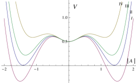
Figure 1: The shape of the scalar potential (63) in units of $g^{2}\xi$ for $\tilde{L}$ given in (66) for various values of the parameter $k$. I. $k=3.6\,\xi$,  II. $k=3.37\,\xi$,  III. $k=3.2\,\xi$,  IV. $k=2.8\,\xi$

As a second example, we can take

$$K=\ln(1+a\bar{a})$$ (67)

for the Kähler potential, and

$$D^{(1)}=\frac{1}{2}\frac{a+\bar{a}}{(1+a\bar{a})},\ \ D^{(2)}=-\frac{i}{2}\frac{a-\bar{a}}{(1+a\bar{a})},\ \ D^{(3)}=-\frac{1}{2}\left(\frac{1-a\bar{a}}{1+a\bar{a}}\right)$$ (68)

for the $S^{2}=SU(2)/U(1)$ Killing potentials. In this case we get that

$$g_{a\bar{a}}=\frac{1}{(1+a\bar{a})^{2}}\,,~{}~{}~{}~{}{\cal{R}}_{a\bar{a}a\bar{a}}=-\frac{2}{(1+a\bar{a})^{4}}$$ (69)

. Then, for a constant positive parameter $m$ and

$$\tilde{{\cal{U}}}=mg_{A\bar{A}}g_{A\bar{A}},$$ (70)

by using that

$$\left({\cal{D}}^{(1)}\right)^{2}+\left({\cal{D}}^{(2)}\right)^{2}+\left({\cal{D}}^{(3)}\right)^{2}=\frac{1}{2}$$ (71)

we find that the scalar potential turns out to be

$${\cal{V}}_{S^{2},EP}=\frac{1}{4}g^{2}-\frac{1}{64m}\,.$$ (72)

From (72) we see that the only effect of the uplifted emerging potential is to inherit the theory with some cosmological constant, depending on the parameters $\xi$, $g$ and $m$.

4.2 Emergent Potential for Two Chiral Multiplets with no Superpotential

We now introduce a second chiral multiplet, but still no superpotential. The only restriction we place on the Kähler potential is that it has the form

$$K=K_{1}(\Phi_{1},\bar{\Phi}_{1})+K_{2}(\Phi_{2},\bar{\Phi}_{2})+d$$ (73)

with $K_{1}$ and $K_{2}$ hermitian functions of $\Phi_{1},\bar{\Phi}_{1}$ and $\Phi_{2},\bar{\Phi}_{2}$, respectively. Moreover we shall restrict the higher derivative scalar couplings to the simple form

$${\tilde{\Lambda}}_{i\bar{r}j\bar{n}}=m\tilde{K}_{i\bar{r}}\tilde{K}_{j\bar{n}}\,,$$ (74)

with $m$ some positive definite function of the superfields that respects the gauged isometries. The equations for the two auxiliaries $F^{1}$ and $F^{2}$ are

$$16g_{2\bar{2}}\ y\ {\tilde{D}}_{a}A^{2}{\tilde{D}}^{a}\bar{A}^{\bar{1}}\!-\!32e^{\frac{K}{3}}x\!+\!16g_{j\bar{n}}{\tilde{D}}_{a}A^{j}{\tilde{D}}^{a}\bar{A}^{\bar{n}}\!+\!16g_{1\bar{1}}{\tilde{D}}_{a}A^{1}{\tilde{D}}^{a}\bar{A}^{\bar{1}}=-m^{-1},$$

$$16g_{1\bar{1}}\ \frac{1}{y}\ {\tilde{D}}_{a}A^{1}{\tilde{D}}^{a}\bar{A}^{\bar{2}}\!-\!32e^{\frac{K}{3}}x\!+\!16g_{j\bar{n}}{\tilde{D}}_{a}A^{j}{\tilde{D}}^{a}\bar{A}^{\bar{n}}\!+\!16g_{2\bar{2}}{\tilde{D}}_{a}A^{2}{\tilde{D}}^{a}\bar{A}^{\bar{2}}=-m^{-1}$$ (75)

where we have defined

$$x=g_{j\bar{n}}F^{j}\bar{F}^{\bar{n}}\,,~{}~{}~{}y=\frac{\bar{F}^{\bar{2}}}{\bar{F}^{\bar{1}}}.$$ (76)

Equations (4.2) can be combined in order to provide a solution for $x$ which is found to be

$$x= \frac{1}{4}e^{\frac{-K}{3}}\left(\frac{1}{8m}+3g_{j\bar{n}}{\tilde{D}}_{a}A^{j}{\tilde{D}}^{a}\bar{A}^{\bar{n}}\right)$$

$$\pm\frac{1}{4}e^{\frac{-K}{3}}\left\{\Big{(}g_{1\bar{1}}{\tilde{D}}_{a}A^{1}{\tilde{D}}^{a}\bar{A}^{\bar{1}}-g_{2\bar{2}}{\tilde{D}}_{a}A^{2}{\tilde{D}}^{a}\bar{A}^{\bar{2}}\Big{)}^{2}\right.$$

$$\left.\ \ \ \ \ \ \ \ \ \ \ \ +4g_{1\bar{1}}g_{2\bar{2}}{\tilde{D}}_{a}A^{2}{\tilde{D}}^{a}\bar{A}^{\bar{1}}{\tilde{D}}_{b}A^{1}{\tilde{D}}^{b}\bar{A}^{\bar{2}}\right\}^{\frac{1}{2}}.$$

Then, plugging back into the action (4), the on-shell theory is

$$e^{-1}{\cal{L}}_{tot}= -\frac{1}{2}R-\frac{1}{4}g_{i{\bar{r}}}{\tilde{D}}_{a}A^{i}{\tilde{D}}^{a}\bar{A}^{\bar{r}}-\frac{1}{16g^{2}}F_{cd}^{(a)}F^{cd(a)}+\frac{1}{64m}-\frac{1}{2}g^{2}\left({\cal{D}}^{(a)}\right)^{2}$$ (78)

$$+9m\Big{(}g_{i{\bar{r}}}{\tilde{D}}_{a}A^{i}{\tilde{D}}^{a}\bar{A}^{\bar{r}}\Big{)}^{2}-16mg_{i{\bar{r}}}g_{j{\bar{n}}}{\tilde{D}}_{a}A^{i}{\tilde{D}}^{a}A^{j}{\tilde{D}}_{b}\bar{A}^{\bar{r}}{\tilde{D}}^{b}\bar{A}^{\bar{n}}$$

$$+4mg_{1\bar{1}}g_{2\bar{2}}{\tilde{D}}_{a}A^{2}{\tilde{D}}^{a}\bar{A}^{\bar{1}}{\tilde{D}}_{b}A^{1}{\tilde{D}}^{b}\bar{A}^{\bar{2}}+m\Big{(}g_{1\bar{1}}{\tilde{D}}_{a}A^{1}{\tilde{D}}^{a}\bar{A}^{\bar{1}}-g_{2\bar{2}}{\tilde{D}}_{a}A^{2}{\tilde{D}}^{a}\bar{A}^{\bar{2}}\Big{)}^{2}$$

$$\pm\Big{(}\frac{1}{4}+6mg_{i{\bar{r}}}{\tilde{D}}_{a}A^{i}{\tilde{D}}^{a}\bar{A}^{\bar{r}}\Big{)}\left\{\Big{(}g_{1\bar{1}}{\tilde{D}}_{a}A^{1}{\tilde{D}}^{a}\bar{A}^{\bar{1}}-g_{2\bar{2}}{\tilde{D}}_{a}A^{2}{\tilde{D}}^{a}\bar{A}^{\bar{2}}\Big{)}^{2}\right.$$

$$\left.\!\!\!\phantom{\Big{)}^{2}}+4g_{1\bar{1}}g_{2\bar{2}}{\tilde{D}}_{a}A^{2}{\tilde{D}}^{a}\bar{A}^{\bar{1}}{\tilde{D}}_{b}A^{1}{\tilde{D}}^{b}\bar{A}^{\bar{2}}\right\}^{\frac{1}{2}}$$

where we notice that the minimal kinetic terms have not dissapeared and a number of DBI-like kinetic terms have appeared in the action along with the higher derivatives. The interchanging $\pm$ signs inside the Lagrangian are a manifestation of the higher derivative (safe nevertheless) nature of this supersymmetric theory, due to which, there exists the possibility to have more than one solutions for the auxiliary fields. The interesting part is that the potential of this theory is still the uplifted emergent potential (57), thus, with a suitable choice of the Kähler and Killing potentials one can achieve the various properties discussed earlier. For example, for a $U(1)$ gauged isometry we have

$$K=a_{1}\bar{a}_{\bar{1}}+a_{2}\bar{a}_{\bar{2}}+d\,,~{}~{}~{}~{}D^{(1)}=a_{1}\bar{a}_{\bar{1}}+a_{2}\bar{a}_{\bar{2}}+\xi\,,$$ (79)

with the scalar potential given by

$${\cal{V}}=\frac{1}{2}g^{2}\left(A_{1}\bar{A}_{\bar{1}}+A_{2}\bar{A}_{\bar{2}}+\xi\right)^{2}-\frac{1}{64m}$$ (80)

where $m$ can be a positive constant or a gauge invariant positive definite hermitian function of the fields $A^{1},\bar{A}^{\bar{1}}$ and $A^{2},\bar{A}^{\bar{2}}$.

Summarizing, the well-known standard form of the ${\cal{N}}=1$ potential (4) is only valid at the leading two-derivative level. Whenever higher-derivatives are introduced, an emerging scalar potential appear even when there is no superpotential. The emerging potential is negative defined and can be uplifted to positive values in gauge chiral models by D-term contributions. There are many open problems to be discussed in the future among which is the possible applications of our findings to High Energy phenomenology.

- (1) M. Ostrogradski, 1850 Memoires sur les equations differentielles relatives au probleme des isoperimetres Mem. Ac. St. Petersburg, VI Series, Vol. 4 385 517; R. P. Woodard, “Avoiding dark energy with 1/r modifications of gravity,” Lect. Notes Phys. 720 (2007) 403-433. [astro-ph/0601672].
- (2) G. W. Horndeski, Int. J. Theor. Phys. 10, 363 (1974).
- (3) A. Nicolis, R. Rattazzi and E. Trincherini, “The Galileon as a local modification of gravity,” Phys. Rev. D 79, 064036 (2009) arXiv:0811.2197 [hep-th].
- (4) C. Deffayet, G. Esposito-Farese and A. Vikman, “Covariant Galileon,” Phys. Rev. D 79, 084003 (2009) arXiv:0901.1314 [hep-th].
- (5) C. W. Misner, K. S. Thorne and J. A. Wheeler, “Gravitation,” San Francisco 1973.
- (6) S. Cecotti, S. Ferrara, L. Girardello and M. Porrati, “Lorentz Chern-simons Terms In N=1 Four-dimensional Supergravity Consistent With Supersymmetry And String Compactification,” Phys. Lett. B 164, 46 (1985).
- (7) S. Cecotti, S. Ferrara, L. Girardello, A. Pasquinucci and M. Porrati, “Matter Coupled Supergravity With Gauss-bonnet Invariants: Component Lagrangian And Supersymmetry Breaking,” Int. J. Mod. Phys. A 3, 1675 (1988).
- (8) F. Farakos, C. Germani, A. Kehagias and E. N. Saridakis, “A New Class of Four-Dimensional N=1 Supergravity with Non-minimal Derivative Couplings,” JHEP 1205, 050 (2012) arXiv:1202.3780 [hep-th].
- (9) C. Armendariz-Picon, T. Damour and V. F. Mukhanov, “k - inflation,” Phys. Lett. B 458, 209 (1999) [hep-th/9904075].
- (10) C. Armendariz-Picon, V. F. Mukhanov and P. J. Steinhardt, “Essentials of k essence,” Phys. Rev. D 63, 103510 (2001) [astro-ph/0006373].
- (11) C. Armendariz-Picon, V. F. Mukhanov and P. J. Steinhardt, “A Dynamical solution to the problem of a small cosmological constant and late time cosmic acceleration,” Phys. Rev. Lett. 85, 4438 (2000) [astro-ph/0004134].
- (12) S. Cecotti, “Higher Derivative Supergravity Is Equivalent To Standard Supergravity Coupled To Matter,” Phys. Lett. B 190, 86 (1987).
- (13) S. J. Gates, Jr., “Why auxiliary fields matter: The Strange case of the 4-D, N=1 supersymmetric QCD effective action,” Phys. Lett. B 365, 132 (1996) [hep-th/9508153].
- (14) J. Khoury, J. -L. Lehners and B. A. Ovrut, “Supersymmetric Galileons,” Phys. Rev. D 84, 043521 (2011) [arXiv:1103.0003 [hep-th]].
- (15) J. Khoury, J. -L. Lehners and B. Ovrut, “Supersymmetric P(X,) and the Ghost Condensate,” Phys. Rev. D 83, 125031 (2011) arXiv:1012.3748 [hep-th].
- (16) D. Baumann and D. Green, “Supergravity for Effective Theories,” JHEP 1203, 001 (2012), arXiv:1109.0293 [hep-th].
- (17) M. Koehn, J. -L. Lehners and B. A. Ovrut, “Higher-Derivative Chiral Superfield Actions Coupled to N=1 Supergravity,” arXiv:1207.3798 [hep-th].
- (18) S. Cecotti, S. Ferrara and L. Girardello, “Structure Of The Scalar Potential In General N=1 Higher Derivative Supergravity In Four-dimensions,” Phys. Lett. B 187, 321 (1987).
- (19) J. Wess and J. Bagger, “Supersymmetry and supergravity,” Princeton, USA: Univ. Pr. (1992) 259 p
- (20) B. Zumino, “Supersymmetry and Kahler Manifolds,” Phys. Lett. B 87, 203 (1979).
- (21) S. Kachru, R. Kallosh, A. D. Linde and S. P. Trivedi, “De Sitter vacua in string theory,” Phys. Rev. D 68, 046005 (2003) [hep-th/0301240].
- (22) G. Villadoro and F. Zwirner, “De-Sitter vacua via consistent D-terms,” Phys. Rev. Lett. 95, 231602 (2005) [hep-th/0508167].
- (23) F. Catino, G. Villadoro and F. Zwirner, “On Fayet-Iliopoulos terms and de Sitter vacua in supergravity: Some easy pieces,” JHEP 1201, 002 (2012) arXiv:1110.2174 [hep-th].
- (24) N. Dragon, U. Ellwanger and M. G. Schmidt, “Supersymmetry And Supergravity,” Prog. Part. Nucl. Phys. 18, 1 (1987).
- (25) S. Cecotti, S. Ferrara and L. Girardello, “Flat Potentials In Higher Derivative Supergravity,” Phys. Lett. B 187, 327 (1987).
- (26) N. V. Krasnikov, A. B. Kyiatkin and E. R. Poppitz, “Structure Of The Effective Potential In Supersymmetric Theories With Higher Order Derivatives Coupled To Supergravity,” Phys. Lett. B 222, 66 (1989).
- (27) S. Cecotti, S. Ferrara, L. Girardello, M. Porrati and A. Pasquinucci, “Matter Coupling In Higher Derivative Supergravity,” Phys. Rev. D 33, 2504 (1986).
- (28) S. Sasaki, M. Yamaguchi and D. Yokoyama, “Supersymmetric DBI inflation,” arXiv:1205.1353 [hep-th].
- (29) C. Germani, “Spontaneous Localization on a Brane: a High-Energy Resolution of Braneworlds,” arXiv:1109.3718 [hep-th].
- (30) B. de Wit, S. Katmadas and M. van Zalk, “New supersymmetric higher-derivative couplings: Full N=2 superspace does not count!,” JHEP 1101, 007 (2011) arXiv:1010.2150 [hep-th].
- (31) S. Ferrara and B. Zumino, “Supergauge Invariant Yang-Mills Theories,” Nucl. Phys. B 79, 413 (1974).
- (32) J. A. Bagger, “Coupling the Gauge Invariant Supersymmetric Nonlinear Sigma Model to Supergravity,” Nucl. Phys. B 211, 302 (1983).
- (33) E. Cremmer, S. Ferrara, L. Girardello and A. Van Proeyen, “Coupling Supersymmetric Yang-Mills Theories to Supergravity,” Phys. Lett. B 116, 231 (1982).
- (34) E. Cremmer, S. Ferrara, L. Girardello and A. Van Proeyen, “Yang-Mills Theories with Local Supersymmetry: Lagrangian, Transformation Laws and SuperHiggs Effect,” Nucl. Phys. B 212, 413 (1983).