Hysteresis and thermal limit cycles in MRI simulations of accretion discs

Abstract

The recurrent outbursts that characterise low-mass binary systems reflect thermal state changes in their associated accretion discs. The observed outbursts are connected to the strong variation in disc opacity as hydrogen ionises near 5000 K. This physics leads to accretion disc models that exhibit bistability and thermal limit cycles, whereby the disc jumps between a family of cool and low accreting states and a family of hot and efficiently accreting states. Previous models have parametrised the disc turbulence via an alpha (or ‘eddy’) viscosity. In this paper we treat the turbulence more realistically via a suite of numerical simulations of the magnetorotational instability (MRI) in local geometry. Radiative cooling is included via a simple but physically motivated prescription. We show the existence of bistable equilibria and thus the prospect of thermal limit cycles, and in so doing demonstrate that MRI-induced turbulence is compatible with the classical theory. Our simulations also show that the turbulent stress and pressure perturbations are only weakly dependent on each other on orbital times; as a consequence, thermal instability connected to variations in turbulent heating (as opposed to radiative cooling) is unlikely to operate, in agreement with previous numerical results. Our work presents a first step towards unifying simulations of full MHD turbulence with the correct thermal and radiative physics of the outbursting discs associated with dwarf novae, low-mass X-ray binaries, and possibly young stellar objects.

1 Introduction

Recurrent outbursts in accreting systems are commonly attributed to global instabilities in their associated accretion discs. In particular, it is believed that thermal instability driven by strong variations in the disc’s cooling rate causes the observed state transitions in dwarf novae (DNe) and low-mass X-ray binaries (LMXBs) (Lasota 2001), while the rich array of accretion variability associated with quasars could be excited by thermal instability driven by variations in the turbulent heating rate (Shakura and Sunyaev 1976, Abramowicz et al. 1988), by thermal-viscous instability (Lightman & Eardley 1974), or assorted dynamical instabilities (e.g. Papaloizou & Pringle 1984, Kato 2003, Ferreira & Ogilvie 2009). On the other hand, FU Ori outbursts, characteristic of protostellar discs, probably result from the interplay of thermal, gravitational, and magnetorotational instability (MRI) across the intermittently inert dead zone (Gammie 1996, Balbus & Hawley 1998, Armitage et al. 2002, Zhu et al. 2009, 2010). Exceptions to this class of model include classical novae whose outbursts can be traced to thermonucleur fusion of accreted material on the white dwarf surface (Gallagher & Starrfield 1978, Shara 1989, Starrfield et al. 2000).

The most developed, and possibly most successful, model of accretion disc outbursts describes the recurrent eruptions that characterise the light curves of DNe and LMXBs. In this model, the ionisation of hydrogen, occurring at temperatures of around 5000 K, induces a significant opacity change in the disc orbiting the primary star (Faulkner et al. 1983, hereafter FLP83), which then leads to thermal instability and hysteresis in the disc gas (Pringle 1981). The system exhibits a characteristic ‘S-curve’ in the phase plane of surface density $\Sigma$ and central temperature $T_{c}$ (cf. Fig. 1), and as a consequence the gas falls into one of two stable states: an optically thick hot state, characterized by strong accretion, or an optically thin cooler state, in which accretion is less efficient (e.g. Meyer & Meyer-Hofmeister 1981, FLP83). Outbursts can then be modelled via a ‘limit cycle’, whereby the disc jumps from the low accreting state to the high accreting state and then back again as mass builds up and is then evacuated. This mechanism, based on local bistable equilibria, is the foundation for a variety of advanced models, which have enjoyed significant successes in reproducing the observed behaviour of accretion discs in binary systems, even if interesting discrepancies persist (Lasota 2001).

The classical model of DNe and LMXBs treats the disc as laminar and assumes that the disc turbulence can be modelled with the $\alpha$ prescription (Shakura & Sunyaev 1973), whereby the action of the turbulent stresses is characterized as a diffusive process with an associated ‘eddy’ viscosity (Balbus & Papaloizou 1999). This has been sufficient to sketch out the qualitative features of putative outbursts, but such a crude description has imposed limitations on the formalism that are now impeding further progress (Lasota 2012). On the other hand, fully consistent magnetohydrodynamic (MHD) simulations of disc turbulence generated by the MRI have been performed for almost 20 years (Hawley et al. 1995, Stone et al. 1996, Hawley 2000, etc), though typically with simplified thermodynamics (e.g. isothermality). It is the task of this paper to begin the process of uniting the classic thermal instability models of DNe and LMXBs with full MHD simulations of the MRI, and thus consistently account for both the turbulence and radiative cooling. The first step we take is limited to local models, as even though discs undergo global outbursts, the ability of local annuli to exhibit hysteresis behaviour is key. Local studies will permit us to assess if and how the classic model of thermal instability can operate in the presence of realistic turbulent heating. At the same time, they provide an excellent test of the MRI itself; if the MRI is to remain the chief candidate driving disc accretion it must fulfil its obligations to classical disc theory.

We undertake unstratified shearing box simulations of the MRI that include Ohmic and viscous heating and a radiative cooling prescription that is able to mimic the transition between the optically thin and thick states (FLP83). These simulations clearly reproduce S-curves in the $\Sigma$ and mean temperature plane, and these constitute the main result of our paper. We can thus animate local thermal limit cycles via a sequence of local box runs. In particular, the simulated turbulent heating is found to be ‘well-behaved’ and not so intermittent as to prematurely disrupt the thermal limit cycles required by the classical theory. In addition, simulations with differing net toroidal and vertical fluxes produce S-curves that exhibit variable mean values of $\alpha$, suggesting that when global simulations are considered, and net-flux is no longer conserved locally, variations in effective $\alpha$ between the upper and lower branches of the S-curve may be produced, as required by the classical model (e.g. Smak 1984a).

Finally, the simulated short-term behaviours of the average viscous stress and the disc pressure reveal only a weak functional dependence, as remarked upon by previous authors (Hirose et al. 2009). This poor correlation means that proposed thermal instabilities driven by a direct heating response to imposed pressure perturbations are unlikely to function in radiation-pressure dominated accretion discs (e.g. Shakura & Sunyaev 1976, Abramowicz et al. 1988). This is in marked contrast to the thermal instabilities implicated in DNe and LMXBs, which are driven by the cooling response to imposed temperature perturbations, mediated via opacity variations. Note, however, that over long times we find that the stress and pressure are correlated.

The plan of the paper is as follows. In the following section we discuss the thermal instability model for DNe and LMXBs in more detail. In Section 3 we present the governing equations while outlining the radiative cooling prescription the simulations adopt. In section 4 we give the numerical details of the simulations. Our results are presented in Section 5, and we conclude in Section 6.

2 Background

We consider close binary systems that consist of one low-mass lobe-filling star transferring material to a degenerate companion, either a white dwarf or a black-hole/neutron star. The characteristic feature of these systems is their recurrent eruptive activity in the optical or X-ray spectrum, respectively. DNe undergo outbursts of some 2-5 magnitude which last 2-20 days, with recurrence intervals ranging from 10 days to years (see e.g. Warner 1995). In addition, certain sources exhibit more complex behaviour, such as ‘superoutbursts’ and ‘standstills’ (whereby the cycle is interrupted for an indefinite period). LMXBs are poorly constrained relative to DNe because they emit almost exclusively in X-rays, and so do not enjoy the same observational coverage. Even so, it has been established that their outbursts exhibit luminosity enhancements of several orders of magnitude, while their spectra progress through a series of canonical X-ray states (McClintock and Remillard 2006).

It is generally accepted that outbursts in these systems take place in the accretion disc that orbits around the primary star and are triggered once sufficient mass has built up in the disc. During an outburst the disc jumps from a cool low-accreting state to a hot high-accreting state that deposits this surfeit of material onto the central object. After this mass has been evacuated the disc returns to its low state and the cycle repeats. The basic outline of the model was first proposed by Smak (1971) and Osaki (1974); but the physical basis for instability in the disc was not understood till much later (FLP83, see also Hoshi 1979). Researchers now recognise that the cycles are the consequence of a thermal instability related to the variation of opacity with temperature.

Above roughly $5000$K the collisional ionisation of hydrogen commences, and this liberates an increasing number of free electrons that enhance the gas opacity $\kappa$. The dependence of opacity on temperature, for a range of densities, is conveniently illustrated in Fig. 9 of Bell & Lin (1994). The figure shows that, after ionisation of hydrogen is complete $T\gtrsim 10^{4}$K, we have roughly $\kappa\propto T^{-2.5}$, and thus $\kappa$ decreases with temperature. On the other hand, cold molecular gas, with $T\lesssim 2\times 10^{3}$K, exhibits a $\kappa$ that also decreases with temperature, primarily on account of dust grain destruction. But the gas opacity in the intermediate temperature regime between these two limits increases rapidly with temperature, because of the flood of free electrons. Here $\kappa\propto T^{10}$, approximately. This dramatic tendency for heat to be better trapped as temperature increases leads immediately to thermal instability in this regime.

The instability criterion can be formulated quantitatively via the following argument. Let us denote by $\epsilon_{D}$ the local turbulent dissipation rate per unit area. Then local thermal equilibrium is determined by balancing this injection rate against the disc’s radiative losses:

$$\epsilon_{D}=2\sigma T_{e}^{4},$$ (1)

where $T_{e}$ is the effective temperature of the disc’s photosphere and $\sigma$ is Stefan’s constant. If we now denote by $T_{c}$ the midplane temperature of the disc, a local thermal stability criterion for this state is simply:

$$\frac{d\epsilon_{D}}{dT_{c}}<2\frac{d\sigma T_{e}^{4}}{dT_{c}},$$ (2)

(Lasota 2001). This expresses the requirement that when the midplane temperature $T_{c}$ is increased, the cooling response via radiation must outstrip the increase in the heating. If this condition is not met, then the midplane temperature increase will be reinforced and there will be a thermal runaway.

At high temperatures, well above the ionisation threshold, we find that the disc radiates efficiently and that $d\ln T_{e}^{4}/d\ln T_{c}\approx 7$. The heating rate $\epsilon_{D}$, on the other hand, increases much more slowly ($\propto T_{c}$ for a laminar $\alpha$ model) and so thermal stability ensues. However, in the transition regime, where $4\times 10^{3}<T\lesssim 10^{4}$ K, the photospheric temperature $T_{e}$ varies very weakly with $T_{c}$ because the opacity is increasing rapidly. The cooling rate barely responds to an increase in central temperature $T_{c}$, which leads to the trapping of excess heat and thermal instability. At the lowest temperatures, $T\lesssim 4000$K, stability is recovered because the disc enters an optically thin regime in which the rate of surface radiation increases rapidly with $T_{c}$. In summary, the disc is bistable and will tend to move to one of two thermally stable steady regimes: (a) hot and ionised (hence efficiently accreting), with $T>10^{4}$K; or (b) cold and predominantly neutral (less efficiently accreting) with $T<4000$K. In addition, there exists an unstable intermediate equilibrium state between these two limits.

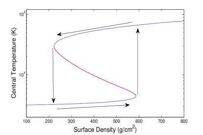
Figure 1: Representative plot of an S-curve defining local steady state thermal equilibria with limit cycle arrows. This is constructed from the laminar $\alpha$ disc modelling of FLP83. For reference the parameters were $E=3.5$, $\lambda=5$, $\mu=1$, and $\alpha_{\text{SS}}=0.0275$ (see Section 3 and the Appendix). We remark that in this figure, central temperature is plotted as ordinate. However, if the mass flow rate ${\dot{M}}$ is used instead, a curve of the same qualitative form results (FLP83).

Because for a given surface density $\Sigma$ there can be up to three $T_{c}$ associated with a thermal equilibrium, the family of equilibrium solutions sketches out a characteristic S-curve in either the $(\Sigma,\,T_{c})$ plane or, alternatively, the $(\Sigma,\,{\dot{M}})$ plane, where $\dot{M}$ is mass accretion rate. Note that $\dot{M}$ can be directly related to $T_{c}$ and $\Sigma$ (e.g. see FLP83 and section 4.2 below). In Fig. 1, we plot a representative family of such thermal equilibria in the $(\Sigma,\,T_{c})$ plane computed via the techniques of FLP83. There is a range of $\Sigma$ for which the system supports three states, two stable (indicated with a blue colour), one unstable (indicated with a red colour).

In Fig. 1 the trajectory of the outbursting limit cycle is represented by the black arrows. Consider gas physically located at the outermost disc radii and in a thermodynamic state associated with the lower branch. At this radius, mass steadily accumulates because accretion onto the primary star cannot match the mass transfer into the disc from the secondary. Consequently, the surface density increases and we travel up the lower branch until it ends, at which point the gas heats up dramatically. Once it settles on the upper branch accretion is much more efficient and a transition wave propagates through the disc (Papaloizou et al. 1983, Meyer & Meyer-Hofmeister 1984, Smak 1984a). Provided conditions are favourable and the front propagates inwards, converting the entire disc into an upper state, there will be a global outburst that results in a significant mass deposit onto the primary. Consequently, the surface density everywhere decreases until the disc undergoes a downward transition to the lower branch.

Our discussion of the thermal equilibria and limit cycles need only consider local models of an accretion disc. However, more advanced DN and LMXB models must incorporate additional global physics in order to capture the heating and cooling fronts that mediate branch changes, and ultimately to match specific observations in detail (e.g. Papaloizou et al. 1983, Smak 1984b, Ichikawa & Osaki 1992, Menou et al. 1999). Even so, all such global treatments are founded on the hysteresis behaviour of the local model (single annulus) outlined above. In this paper we concentrate on this fundamental engine of instability. Our aim is to show that it can function in the presence of turbulence generated by the MRI. This is intended as a first step in moving disc outburst modelling away from the heuristic $\alpha$ prescription. Future work can then include the detailed global physics.

3 Governing equations

We adopt the local shearing box model (Goldreich & Lynden-Bell, 1965) and a Cartesian coordinate system $(x,y,z)=(x_{1},x_{2},x_{3})$ with origin at the centre of the box. These coordinates represent the radial, azimuthal, and vertical directions respectively. Vertical stratification is neglected. The basic equations express the conservation of mass, momentum, and energy and include the induction equation for the magnetic field. They incorporate a constant kinematic viscosity $\nu$ and magnetic diffusivity $\eta.$ The continuity equation, equation of motion, and induction equations are given by

$$\frac{\partial\rho}{\partial t}+\mbox{\boldmath{$\nabla$}}\mbox{\boldmath{$\cdot$}}(\rho\mbox{\boldmath{$v$}})=0\,,$$ (3)

$$\rho\left(\frac{D\mbox{\boldmath{$v$}}}{Dt}+2\mbox{\boldmath{$\Omega$}}\times\mbox{\boldmath{$v$}}+\mbox{\boldmath{$\nabla$}}\Phi\right)=\frac{(\mbox{\boldmath{$\nabla$}}\mbox{\boldmath{$\times$}}\mbox{\boldmath{$B$}})\mbox{\boldmath{$\times$}}\mbox{\boldmath{$B$}}}{4\pi}-\mbox{\boldmath{$\nabla$}}P+\nabla\mbox{\boldmath{$\cdot$}}\mathbf{\Pi},$$ (4)

$$\frac{\partial\mbox{\boldmath{$B$}}}{\partial t}=\mbox{\boldmath{$\nabla$}}\mbox{\boldmath{$\times$}}(\mbox{\boldmath{$v$}}\mbox{\boldmath{$\times$}}\mbox{\boldmath{$B$}}-\eta\mbox{\boldmath{$\nabla$}}\mbox{\boldmath{$\times$}}\mbox{\boldmath{$B$}})\,$$ (5)

and the first law of thermodynamics is written in the form

$$\rho\frac{De}{Dt}-\frac{P}{\rho}\frac{D\rho}{Dt} = \mathbf{\Pi}:\nabla\mbox{\boldmath{$v$}}+\frac{\eta|\mbox{\boldmath{$\nabla$}}\mbox{\boldmath{$\times$}}\mbox{\boldmath{$B$}}|^{2}}{4\pi}-\Lambda.$$ (6)

Here the convective derivative is defined through

$$\frac{D}{Dt} \equiv \frac{\partial}{\partial t}+\mbox{\boldmath{$v$}}\cdot\nabla,$$ (7)

$\Omega$ is the Keplerian orbital frequency evaluated at the centre of the box, $v$ is the velocity, $B$ is the magnetic field and $e$ is the internal energy per unit mass. The tidal potential is $\Phi=-3\Omega^{2}x^{2}/2$ and $\Lambda$ is the (radiative) cooling rate per unit volume. The right hand side of Equation (6) includes contributions from viscous dissipation, Ohmic heating and radiative losses. The components of the viscous stress tensor $\mathbf{\Pi}$ are given by

$$\Pi_{ik}=\rho\nu\left(\frac{\partial v_{i}}{\partial x_{k}}+\frac{\partial v_{k}}{\partial x_{i}}-\frac{2}{3}\delta_{ik}\mbox{\boldmath{$\nabla$}}\mbox{\boldmath{$\cdot$}}\mbox{\boldmath{$v$}}\right)\,,$$ (8)

In addition, the magnetic field must satisfy $\nabla\cdot\mbox{\boldmath{$B$}}=0$. Finally, we adopt an ideal gas equation of state

$$P=\frac{2e}{3}\rho=\rho c_{s}^{2},$$ (9)

where $c_{s}^{2}={\cal R}T/\mu$ is the isothermal sound speed, with $T$ the temperature, ${\cal R}$ the gas constant, and $\mu$ the mean molecular weight.

3.1 Radiative cooling model

In order to proceed, we need to realistically account for the radiative cooling of the gas, via the term $\Lambda$. The shearing box by definition is located far from the disc’s upper and lower surfaces with periodic boundary conditions applied in the vertical direction. Nevertheless, we can approximate the box’s radiative losses in a physically meaningful way via a prescription outlined in FLP83.

Our model assumes that the cooling $\Lambda$ is a function only of time and horizontal position $(x,\,y)$. It is taken to be

$$\Lambda=2\sigma T_{e}^{4}/H_{0},$$ (10)

where $T_{e}$ is interpreted as the effective temperature at the upper and lower vertical boundary of the disc. Here $H_{0}$ is a reference scale height. The main task is to derive how the surface temperature $T_{e}$ varies in response to changes in the midplane temperature $T_{c}$.

We envisage that $T_{e}$ takes a different form in three distinct physical disc regimes.

1. The first regime corresponds to the hot optically thick conditions associated with the disc’s high accreting state. In such a state, the disc’s photospheric temperature $T_{e}$ is marginally above the value appropriate for the ionisation threshold for hydrogen ($\sim 5000$ K) and so the entire disc is optically thick. The classical relationship $T_{e}^{4}=(4/3)(T_{c}^{4}/\tau_{c})$, where $\tau_{c}$ is midplane optical depth, can be used to relate $T_{e}$ and $T_{c}.$ As most of the optical depth comes from the regions close to the midplane, $\tau_{c}$ can be evaluated using the midplane opacity.

2. The second regime corresponds to an intermediate ‘hybrid’ state in which the midplane is hot and partially ionised but the surface layers have become sufficiently cool for hydrogen ionisation to fall off sharply. As a consequence, the opacity drops near the photosphere with drastic consequences for the disc’s vertical temperature structure, as in cool stars (Hayashi & Hoshi 1961). The classical dependence of $T_{e}$ on $T_{c}$ breaks down, with the connection between the two becoming quite weak. Instead, we must determine $T_{e}$ from the outer boundary condition $\tau_{e}=1$, where $\tau_{e}$ is photospheric optical depth.

3. The third regime corresponds to the cool optically thin regime in which the entire disc, including the midplane, lies marginally below the ionisation threshold. In this regime, consideration of direct cooling then yields a simple approximate relationship between $T_{c}$ and $T_{e}$.

In the Appendix we consider each regime in turn and obtain three functional forms relating $T_{e}$ to $T_{c}$ and $\Sigma$. Our final expression for $T_{e}$ is an interpolation formula, Eq.  (36), connecting these different regimes. In summary, the prescription for finding $T_{e}$ is given by

$$T_{e}=\begin{cases}\left(4/3\tau_{c}\right)^{1/4}T_{c},&\text{in Regime 1},\\ \left(10^{36}\,E\rho_{c}^{-1/3}/\Sigma\right)^{1/10},&\text{in Regime 2},\\ \left(2\lambda\tau_{c}\right)^{1/4}T_{c},&\text{in Regime 3},\end{cases}$$ (11)

where $E$ and $\lambda$ are two dimensionless constants, and the midplane optical depth is $\tau_{c}=\kappa_{c}\Sigma$ with $\kappa_{c}$ being the opacity evaluated at the midplane density $\rho_{c}$ and temperature $T_{c}$. All dimensional quantities are in cgs units. As in FLP83 the opacity in regime 1 is taken to be

$$\kappa=1.5\times 10^{20}\rho T^{-2.5}$$ (12)

and in regime 3 it is taken to be

$$\kappa=10^{-36}\rho^{1/3}T^{10}.$$ (13)

In addition,

$$\rho_{c}=\frac{\Sigma}{2H}=\frac{\Sigma\,\Omega\,}{2}\left(\frac{\mu}{\mathcal{R}T}\right)^{1/2}.$$ (14)

Finally, we specify a constant $\mu$ for all regimes. This of course neglects partial ionization, but should not interfere especially in our qualitative results.

In FLP83, thermal equilibrium solutions are computed by matching the cooling rate, computed according to the above procedure, with the turbulent alpha heating, for which the volume heating rate is

$$\epsilon_{D}=3\alpha_{\text{SS}}\rho{\cal R}T\Omega/(2\mu),$$ (15)

where the Shakura-Sunyaev $\alpha_{\text{SS}}$ parameter is a dimensionless constant less than one (cf. Eq. (21)). These solutions may be viewed as relations between $\Sigma$ and $T_{c}$, though they are more commonly re-expressed as relations between $\Sigma$ and $T_{e}.$ Some of these S-curves are illustrated in Figs 1 and 4-6.

4 Numerical set-up

We solve equations (3)-(6) with a parallel version of ZEUS (Stone & Norman 1992a, 1992b). This uses a finite difference scheme to obtain the spatial derivatives, is first order explicit in time, and employs constrained transport to ensure $B$ remains solenoidal. Our version of ZEUS has been altered according to improvements outlined by Lesaffre & Balbus (2007), Silvers (2008), and Lesaffre et al. (2009). These simulations are conducted in a shearing box with dimensions $(H_{0},4H_{0},H_{0})$. As a check on the robustness of the main results and to verify their independence on the numerical implementation, some simulations were also performed with NIRVANA (Ziegler 1999, Papaloizou & Nelson 2003) adopting a shearing box with dimensions $(L_{x},L_{y},L_{z})=(H_{0},\pi H_{0},H_{0}).$

The reference scale height is given by

$$H_{0}=\frac{c_{s0}}{\Omega}=\left(\frac{\mathcal{R}T_{0}}{\mu\Omega^{2}}\right)^{1/2}$$ (16)

and thus corresponds to some prescribed isothermal sound speed $c_{s0}$ or, equivalently, temperature $T_{0}$. Note that as the simulations considered here are not isothermal, $c_{s0}$ need not necessarily correspond to the actual sound speed at any location or any time. In practice, however, it often approximates a volume average of the initial average sound speed (for ZEUS runs) or the sound speed under quasi-steady conditions (NIRVANA runs).

The box is periodic in the $x$ and $z$ direction and shearing periodic in the azimuthal $y$ direction (see Hawley et al. 1995). Space is scaled by $H_{0}$ and time is measured in units of $\Omega^{-1}$. Density is measured in terms of the average mass density in the box $\rho_{0}$, and magnetic field by the background field strength $B_{0}$ (see below). Finally, temperature is scaled by $T_{0}$.

The NIRVANA simulations employ a resolution of $(N_{x},N_{y},N_{z})=(128,200,128)$, where $N_{i}$ is the number of grid cells in the $i$’th direction. This resolution level was adopted in Fromang et al. (2007) and Fromang (2010) and was there found to be converged. The ZEUS simulations, on the other hand, adopt a resolution of $(128,512,128)$. Though more demanding, because of the higher resolution in the direction of shear, the ZEUS simulations can take advantage of the numerical benefits of an isotropic grid (Lesaffre & Balbus 2007). Additional runs were performed with the resolution reduced by a factor of two for both codes and these indicated no significant differences from the main results (see Section 5.4).

In order to study simulations with a range of strengths of turbulent activity, three different magnetic field configurations (and boundary conditions) were implemented: fields with zero net-flux (or zero vertical-flux), fields with net vertical-flux, and fields with net toroidal-flux (see Hawley et al. 1995). In the net field cases, we must stipulate the initial plasma beta of a run:

$$\beta=\frac{8\pi P_{0}}{B_{0}^{2}},$$ (17)

where $B_{0}$ is the strength of the mean field penetrating the box and $P_{0}=\rho_{0}H_{0}^{2}\Omega^{2}$ is the initial pressure. As $\beta$ decreases, simulations become more active and display larger effective values of $\alpha$. Furthermore, the cases with net vertical and with net toroidal flux produce turbulence manifesting similar mean values of $\alpha$ but with different characteristics (Hawley et al. 1995). This can give an indication of to what extent specification of the mean value of $\alpha$ is sufficient to characterize the thermal equilibria.

In the zero flux case, we set the initial vertical field to be of the form $B_{0}\sin(x/H_{0})$. However, provided $B_{0}$ is large enough for the MRI to be resolved, the system attains a state after some 10 orbits that is independent of the initial condition (Balbus & Hawley 1998).

For the diffusivities, we adopted parameters similar to those in Fromang et al. (2007) which compared results for zero flux simulations obtained from three codes, ZEUS, NIRVANA and the PENCIL code. These were found to be consistent and, in subsequent work of Fromang (2010), converged. We remark that Fromang et al. (2007) showed that the level of MRI turbulence critically depends on the magnetic Prandtl number $\mathrm{Pm}=\nu/\eta$, i.e. the ratio of kinematic viscosity to magnetic diffusivity. As a consequence, we set $\mathrm{Pm}=4$ to ensure sustained activity, and take

$$\nu=32\times{}10^{-5}H_{0}^{2}\Omega\quad\text{and}\quad\eta=8\times 10^{-5}H_{0}^{2}\Omega.$$ (18)

Finally, in the case of NIRVANA, the initial data was prepared from similar isothermal simulations to those carried out in Fromang et al. (2007). Heating and cooling is then ‘switched on’ at a given time after a quasi-steady turbulent state is attained. The ZEUS runs begin from large amplitude perturbations which blend a large number of MRI shearing waves, as calculated from the linear theory (Balbus & Hawley 1992). In this way a saturated turbulent state can be achieved relatively quickly and without an initial disruptive transient (Lesaffre et al. 2009).

4.1 Numerical implementation of the radiative cooling model

In this paper we are interested in thermal equilibria generated by models in which heating is provided directly through MRI turbulence. Accordingly, the cooling prescription must be implemented as an algorithm within our simulations. The values for $T_{c}$ that are input into the function $\Lambda$ (see equations (10) and (36)) is taken to be the vertically averaged temperature in the box,

$$T_{c}(x,y,t)=\frac{1}{L_{z}}\int_{0}^{L_{z}}T(x,y,z,t)\,dz,$$ (19)

and thus $\Lambda$ is a function only of $x$, $y$, and time. Consequently, the cooling rate is the same for every $z$ at a given horizontal location $(x,y)$. This is a natural consequence of using a one-zone cooling model of the type we have adopted.

As mentioned earlier, the governing equations that we numerically solve are scaled according to fiducial values for time, space, density, etc. However, when we evaluate the cooling function $\Lambda$, we must convert back to physical dimensions. This means we need to specify explicit values for $\Omega$, $T_{0}$, and $\Sigma$. All calculations were carried out adopting an angular velocity $\Omega$ corresponding to a Keplerian circular orbit of radius $3\times 10^{10}$ cm around a star of mass $1M_{\odot}$. This choice corresponds to the outer regions of an accretion disc around a white dwarf and yield $\Omega=2.22\times 10^{-3}$ s^-1 (FLP83). We explored, however, a range of values for the temperature scale $T_{0}$ and $\Sigma$, over separate simulations, in order to sketch out the various thermal equilibria in the phase space of these variables. The values were chosen so that the simulation begins near an estimated point on an S-curve calculated from an alpha-disc model. Once $\Lambda$ is calculated in dimensional units it is rescaled to simulation units and fed into the energy equation (6). In most cases, simulations remain in the same phase space neighbourhood. However departures can occur in cases where there is a thermal runaway (i.e. no nearby equilibrium). In some cases the box dimensions become mismatched to the physical conditions, at which point the simulation was terminated.

While $T_{0}$ and $\Sigma$ varied considerably, we employed two parameter sets for $(\mu,E,\lambda)$. The first set, corresponds to: $\mu=1$, $E=3.5$, $\lambda=5$. We refer to these as ‘Set 1’. The second set was that adopted by FLP83: $\mu=0.5$, $E=5.66$, and $\lambda=1$. We refer to these as ‘Set 2’. We choose two sets to extend the range of possible disc states and also display the insensivity of our qualitative results to these parameters.

4.2 Diagnostics

Of central importance in our simulations are the turbulent stresses which, via the transport of angular momentum, facilitate mass accretion and localised heating (see Balbus & Papaloizou 1999). We measure the stresses via the turbulent alpha:

$$\alpha=\frac{\langle T_{xy}\rangle}{\langle P\rangle}\equiv\frac{\langle\rho v_{x}v_{y}-B_{x}B_{y}/(4\pi)\rangle}{\langle P\rangle}$$ (20)

where $T_{xy}$ is the $xy$ component of the total turbulent stress tensor and the angle brackets indicate a box average. This is a quantity that fluctuates in time, and thus must be distinguished from the (constant) Shakura-Sunyaev alpha parameter $\alpha_{\text{SS}}$ that is used in laminar disc modelling, defined through

$$\rho\nu=\frac{2}{3}\alpha_{\text{SS}}\,\frac{P}{\Omega}.$$ (21)

The two quantities should coincide once the turbulent alpha is averaged over long times.

The turbulent stresses $T_{xy}$ extract energy from the orbital shear and, once this energy travels down a turbulent cascade, it is thermalised by Ohmic and viscous dissipation. This turbulent heating is captured directly in our model via the first two terms on the right side of (6). In a thermal quasi-steady state this heating rate $\epsilon_{D}$ must balance the radiative cooling rate $\Lambda$. If this is not achieved the temperature of the system $T$ will evolve until a thermal balance is obtained.

In a steady state laminar disc the accretion rate ${\dot{M}}$ is given by

$${\dot{M}}=3\pi{\bar{\nu}}\Sigma,$$ (22)

where ${\bar{\nu}}$ is the vertically averaged value of $\nu$ weighted by density. In a turbulent disc, the equivalent relation employing local averaged quantities is

$${\dot{M}}=\frac{2\pi}{\Omega}\int^{\infty}_{-\infty}\langle T_{r\phi}\rangle dz\approx 2\pi H_{0}\,\frac{\langle T_{xy}\rangle}{\Omega},$$ (23)

and, like $\alpha$, is a time varying quantity.

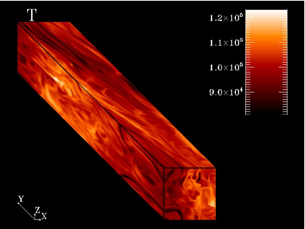
Figure 2: A screen shot of the temperature in Kelvin during a saturated equilibrium state. Parameter Set 1 is used with $\Sigma=1000$ g/cm² with net toroidal field. The upper branch solution has been achieved.

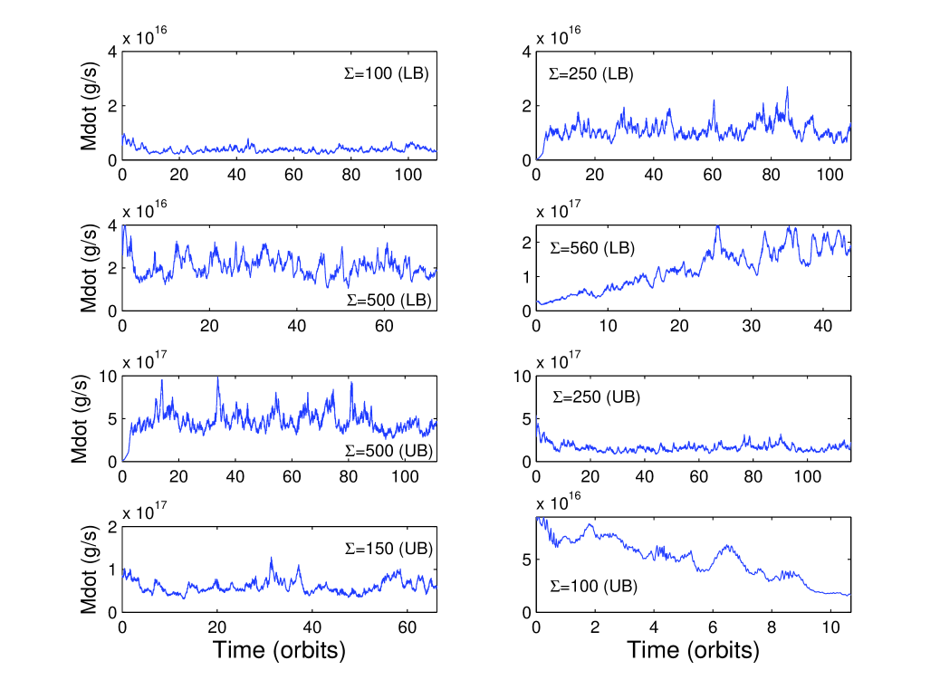
Figure 3: The time evolution of the mass accretion rate $\dot{M}$ in eight simulations for the case of net toroidal-flux and parameter set 1. Here $\beta=100$. Each simulation is distinguished by its (conserved) surface density $\Sigma$ in cgs units. In a sequence running from left to right and top to bottom, the conserved surface density moves first through increasing values for which there is a mean steady state corresponding to the lower branch (LB) of the S-curve plotted in Fig. 4. The simulation that is second from the top and on the right then moves to the upper branch (UB) as there is no available mean steady state on the lower branch. The sequence resumes with states of decreasing surface density tracing out the hot high-accreting solution on the upper branch. The final bottom right simulation then transitions to the lower branch, there being no steady state available on the upper branch for its low $\Sigma$.

5 Numerical results

We undertake numerical simulations of MRI-induced turbulence for two sets of cooling parameters. For each parameter set we investigate three different magnetic configurations: (a) zero-net flux, (b) net-vertical flux, and (c) net-toroidal flux. And for each configuration we conduct a suite of separate simulations with various $(\Sigma,\,T_{0})$ in order to sketch S-curves in each of the 6 cases.

In the net-vertical flux runs, the initial plasma beta is $\beta=10^{4}$. This large value is taken in order to minimise recurrent channel flows — an artefact of small boxes — that may skew our equilibrium results (Hawley et al. 1995, Sano & Inutsuka 2001, Latter et al. 2009). For the net-toroidal flux, stronger fields were employed and the initial beta was either $\beta=50$ or $100.$

Once heating and cooling were activated, each simulation was run until the system had relaxed towards a turbulent thermal equilibrium, if one was nearby, or had monotonically heated up or cooled down so as to change solution branches (cf. the vertical arrows in Fig. 1). In the former cases, the relaxation time depended on the heating rate and hence the magnitude of the turbulent stresses. Because of the small values of $\alpha$ in the zero flux runs, this process could take some time and these runs were typically continued for between 150 and 250 orbits. The net toroidal-flux runs exhibited larger $\alpha$ and a corresponding shorter heating time scale. They required 30 - 100 orbits to reach a quasi-steady states with meaningful statistics. Fig. 2 shows a screen shot of the turbulent vertically-averaged temperature of a representative run once a thermal equilibrium has been achieved. Here a net-toroidal flux simulation has been selected and the upper branch achieved.

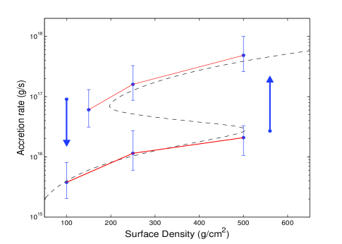
Figure 4: This figure summarises the simulations of Fig. 3 by plotting either their time averaged $\dot{M}$ in the $(\Sigma,\,\dot{M})$ plane, if a thermal equilibrium is achieved, or by showing the initial and end $\dot{M}$ if the simulation exhibits a thermal runaway. Equilibria are plotted as dots with the error bars indicating the range of fluctuations. Runaways are plotted as arrows. Note that despite the range of the fluctuations, equilibria (dots) never flipped between branches. Only simulations begun near branch edges transitioned. The analytic S-curve (dashed), provided for reference, is obtained from following the procedure of FLP83 for $\alpha_{\text{SS}}=0.034.$

In the next subsection we present a collection of 8 runs associated with parameter set 1 and a net-toroidal flux. We show their thermal solution trajectories as functions of time and how these trajectories change as we vary the surface density $\Sigma$. In this way we can trace out individual thermal states along a limit cycle in the $(\Sigma,\,\dot{M})$ plane. Our full set of numerical results are then displayed with a more detailed discussion in the following subsection, where S-curves are sketched out for all magnetic configurations and parameter sets. These, however, are presented in terms of $\Sigma$ and box-averaged temperature. Once this is done we discuss the weak dependence between the turbulent stresses and the heating, and finally issues of numerical convergence.

5.1 Simulation tracks in the $(\Sigma,\,{\dot{M}})$ plane

In laminar disc modelling it is common to describe local S-curves and limit cycles within the phase plane of $\Sigma$ and $\dot{M}$ because it is the accretion rate $\dot{M}$ that dominates the state of the disc. Accordingly, we begin by discussing a subset of our simulation results in terms of the evolution of $\dot{M}$.

In Fig. 3 we plot the evolution tracks of eight simulations with net-toroidal flux, with $\beta=100$, and parameter set 1. The simulations differ in their (conserved) surface density $\Sigma$ and initial temperature $T_{0}$. The simulations achieve either a thermal quasi-steady equilibrium near their initial state, in which $\dot{M}$ fluctuates about a well-defined mean value, or they catastrophically heat up or cool down from their initial state, with an accompanying increase/decrease in $\dot{M}$. These results are summarised by Fig. 4 in the $(\Sigma,\,\langle\dot{M}\rangle)$ plane, where the $\langle\dot{M}\rangle$ of each simulation is computed from a time average over the course of the run. Runs that achieved a thermal steady state near their initial condition are represented as dots with error bars showing the range of the fluctuations in $\dot{M}$. Runs that evolved significantly away from their initial condition are represented by arrows, the base of which denote their starting point and the tip of which their end point when the simulation was terminated.

As we progress from left to right and top to bottom through the eight panels in Fig. 3 we track the S-curve in Fig. 4 starting at the bottom left corner. First we travel towards the right along the lower branch, then up to the higher branch, then to the left along the upper branch, and finally back down to the lower branch. For the first three simulations/panels, the surface density $\Sigma$ moves through increasing values, each of which permits a cool low-accreting equilibrium. But the fourth simulation rapidly migrates from the vicinity of the lower branch: no cool low-accreting steady state is available, because it possesses a $\Sigma$ that is too large. It instead heats up and approaches an upper branch of hot solutions characterised by efficient accretion. The sequence then resumes with a procession of hot equilibria with decreasing $\Sigma$. The eighth simulation transitions from the vicinity of the upper branch to the lower branch as there is no hot high-accreting state available that corrresponds to its low surface density.

Though a single run in local geometry cannot describe a complete limit cycle from beginning to end, our sequence of multiple runs can describe the constituent parts of a cycle, state by state. This is permitted because of the separation of time-scales between the fast turbulent/thermo dynamics that determine the equilibria ($\gtrsim 1/\Omega\sim 10^{3}$ s) and the slow dynamics of the cycle, which is governed by the accretion rate ($\gtrsim 1/(\alpha\Omega)\sim 10^{5}$ s).

Despite the large range of the $\dot{M}$ fluctuations witnessed in Fig. 4 there is never any danger that the equilibrium states spontaneously undergo transitions. States on the lower and upper branches are robust and distinct, with their stability tied to (the smaller) variations in $T$ rather than $\dot{M}$. This point is is more apparent when the S-curves are plotted in the $(\Sigma,\,T)$ plane (see next subsection).

Finally, we have superimposed on Fig. 4 an analytic S-curve computed using the formalism of FLP83 with a Shakura-Sunyaev alpha of $\alpha_{\text{SS}}=0.034$. The location of the two numerical branches and the stable analytic branches is reasonably consistent. However, the numerical branches often seem more extended to the right.

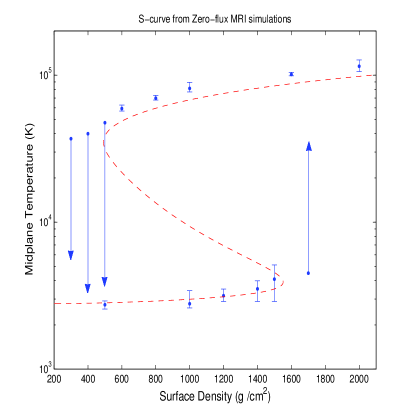
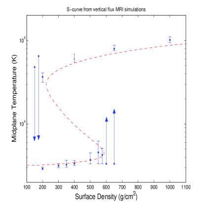
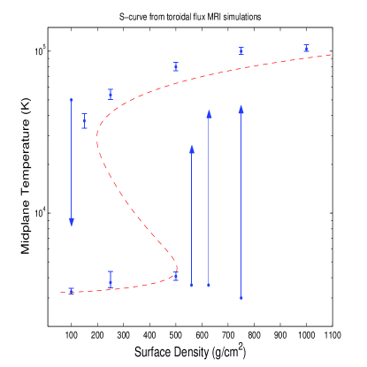
Figure 5: S-curves computed with ZEUS for parameter set 1: $(\mu,E,\lambda)=(1,3.5,5)$ and for the three magnetic configurations. The first panel corresponds to zero net-flux, the second panel to net vertical-flux (initial $\beta=10^{4}$), and the third panel to a net toroidal-flux (initial $\beta=100$). Simulation results are indicated on the $(\Sigma,T_{c})$ plane, with $T_{c}$, in K, evaluated as the volume average of the temperature, $T,$ over the box. $\Sigma$ is expressed in cgs units. Runs that attained an approximate quasi-steady state are indicated by a dot, corresponding to the time average mean volume averaged $T$, and with errorbars, indicating the maximum and minimum volume averaged $T$ once the steady state is achieved. Cases indicated with arrows pointing upward/downward underwent a heating/cooling instability, with the volume averaged $T$ on average showing a monotonic increase/decrease with time. Notation is otherwise the same as in Fig. 4. The dashed curves represent equilibrium S-curves calculated using the formalism of FLP83 for $\alpha_{\text{SS}}=0.007,\,0.0275,\,0.034$ for the zero flux, net-vertical flux, and toroidal flux cases respectively.

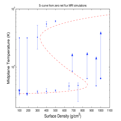
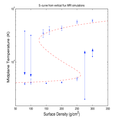
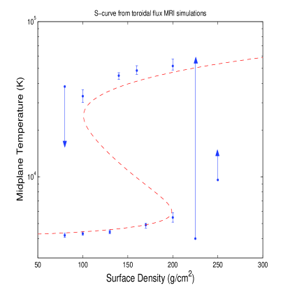
Figure 6: S-curves computed with NIRVANA and ZEUS for the second parameter set: $(\mu,E,\lambda)=(0.5,5.66,1).$ The first panel corresponds to zero net-flux, the second panel to net vertical-flux (initial $\beta=10^{4}$), and the third panel to a net toroidal-flux (initial $\beta=50$). The dashed curves represent equilibrium S-curves calculated using the formalism of FLP83, with $\alpha_{\text{SS}}=0.009,\,0.0475,\,0.07$ for the zero flux, net-vertical flux, and toroidal flux cases respectively. Notation is otherwise the same as in Fig. 5.

Paramater Set 1: Thermal quasi-equilibrium
B Configuration	$\Sigma$	$\langle T\rangle$	max($T$)	min($T$)	$\alpha$	Orbits
Zero Vertical (l.b.)	500	$2.74\times 10^{3}$	$2.91\times 10^{3}$	$2.57\times 10^{3}$	0.0062	240
	1000	$2.79\times 10^{3}$	$3.42\times 10^{3}$	$2.61\times 10^{3}$	$0.0049$	170
	1200	$3.16\times 10^{3}$	$3.51\times 10^{3}$	$2.89\times 10^{3}$	$0.0081$	350
	1400	$3.52\times 10^{3}$	$3.99\times 10^{3}$	$2.89\times 10^{3}$	0.0076	190
	1500	$4.10\times 10^{3}$	$5.12\times 10^{3}$	$2.89\times 10^{3}$	0.0079	300
Zero Vertical (u.b.)	600	$5.92\times 10^{4}$	$6.26\times 10^{4}$	$5.70\times 10^{4}$	0.0084	180
	800	$6.97\times 10^{4}$	$7.30\times 10^{4}$	$6.78\times 10^{4}$	0.0083	90
	1000	$8.14\times 10^{4}$	$8.95\times 10^{4}$	$7.69\times 10^{4}$	0.0098	190
	1600	$10.1\times 10^{4}$	$10.5\times 10^{4}$	$9.83\times 10^{4}$	0.0082	130
	2000	$11.5\times 10^{4}$	$12.7\times 10^{4}$	$10.6\times 10^{4}$	0.010	170
Net Vertical (l.b.)	200	$2.93\times 10^{3}$	$3.05\times 10^{3}$	$2.83\times 10^{3}$	0.0348	80
	300	$3.16\times 10^{3}$	$3.35\times 10^{3}$	$3.00\times 10^{3}$	0.0342	40
	350	$3.25\times 10^{3}$	$3.68\times 10^{3}$	$3.04\times 10^{3}$	0.0359	90
	400	$3.35\times 10^{3}$	$3.68\times 10^{3}$	$3.17\times 10^{3}$	0.0368	80
	500	$3.71\times 10^{3}$	$4.50\times 10^{3}$	$3.33\times 10^{3}$	0.0387	105
	550	$4.56\times 10^{3}$	$6.27\times 10^{3}$	$3.33\times 10^{3}$	0.0384	160
	575	$4.26\times 10^{3}$	$5.09\times 10^{3}$	$3.33\times 10^{3}$	0.0355	100
Net Vertical (u.b.)	200	$3.66\times 10^{4}$	$4.11\times 10^{4}$	$3.16\times 10^{4}$	0.0362	65
	400	$5.99\times 10^{4}$	$6.87\times 10^{4}$	$5.46\times 10^{4}$	0.0351	140
	650	$7.95\times 10^{4}$	$8.79\times 10^{4}$	$7.52\times 10^{4}$	0.0375	48
	1000	$10.1\times 10^{4}$	$11.1\times 10^{4}$	$9.43\times 10^{4}$	0.038	90
Net Toroidal (l.b.)	100	$3.27\times 10^{3}$	$3.44\times 10^{3}$	$3.16\times 10^{3}$	0.0476	110
	250	$3.74\times 10^{3}$	$4.37\times 10^{3}$	$3.46\times 10^{3}$	0.0507	110
	500	$4.01\times 10^{3}$	$4.33\times 10^{3}$	$3.86\times 10^{3}$	0.0422	75
Net Toroidal (u.b.)	150	$3.72\times 10^{4}$	$4.12\times 10^{4}$	$3.35\times 10^{4}$	0.0442	65
	250	$5.36\times 10^{4}$	$5.82\times 10^{4}$	$5.04\times 10^{4}$	0.0487	118
	500	$7.99\times 10^{4}$	$8.53\times 10^{4}$	$7.54\times 10^{4}$	0.0491	110
	750	$9.97\times 10^{4}$	$10.6\times 10^{4}$	$9.52\times 10^{4}$	0.0491	105
	1000	$10.3\times 10^{4}$	$10.9\times 10^{4}$	$9.97\times 10^{4}$	…	65

Table 1: Summary of the inputs and average values of simulations undertaken by ZEUS with parameter set 1: $\mu=1$, $E=3.5$, $\lambda=5$. The magnetic field configuration is varied as is the input surface density $\Sigma.$ The initial $\beta$ is $10^{4}$ for the net vertical field runs, and 100 for the net toroidal field runs. Quasi-steady thermal equilibria are attained that align with one of the two stable branches of the S-curve, with ‘l.b.’ denoting ‘lower branch’, and ‘u.b.’ denoting ‘upper branch’.

Parameter Set 2: Thermal quasi-equilibrium
B Configuration	$\Sigma$	$\langle T\rangle$	max($T$)	min($T$)	$\alpha$	Orbits
Zero Vertical (l.b.)	100	$3.51\times 10^{3}$	$3.65\times 10^{3}$	$3.36\times 10^{3}$	0.0092	120
	300	$3.74\times 10^{3}$	$3.97\times 10^{3}$	$3.51\times 10^{3}$	$0.0095$	180
	400	$3.82\times 10^{3}$	$4.25\times 10^{3}$	$3.50\times 10^{3}$	0.014	334
	500	$3.95\times 10^{3}$	$4.07\times 10^{3}$	$3.74\times 10^{3}$	$0.0095$	123
	650	$4.72\times 10^{3}$	$5.35\times 10^{3}$	$4.07\times 10^{3}$	0.011	197
	750	$4.84\times 10^{3}$	$5.35\times 10^{3}$	$2.55\times 10^{3}$	0.0105	176
Zero Vertical (u.b.)	300*	$3.27\times 10^{4}$	$4.63\times 10^{4}$	$2.04\times 10^{4}$	0.011	211
	300**	$4.64\times 10^{4}$	$5.24\times 10^{4}$	$4.03\times 10^{4}$	0.012	185
	400$\dagger$	$5.52\times 10^{4}$	$5.74\times 10^{4}$	$4.97\times 10^{4}$	0.0095	221
	400$\dagger\dagger$	$5.60\times 10^{4}$	$6.12\times 10^{4}$	$5.09\times 10^{4}$	0.011	226
	500	$6.18\times 10^{4}$	$6.37\times 10^{4}$	$5.98\times 10^{4}$	0.0095	90
Net Vertical (l.b.)	80	$3.90\times 10^{3}$	$4.08\times 10^{3}$	$3.74\times 10^{3}$	0.036	70
	100	$4.11\times 10^{3}$	$4.80\times 10^{3}$	$3.83\times 10^{3}$	0.0425	67
	150	$3.99\times 10^{3}$	$4.06\times 10^{3}$	$3.92\times 10^{3}$	0.038	33
	200	$4.14\times 10^{3}$	$4.24\times 10^{3}$	$4.03\times 10^{3}$	0.041	33
	250	$4.83\times 10^{3}$	$5.19\times 10^{3}$	$4.46\times 10^{3}$	0.042	35
Net Vertical (u.b.)	140	$3.49\times 10^{4}$	$4.08\times 10^{4}$	$2.89\times 10^{4}$	0.045	67
	160	$3.99\times 10^{4}$	$4.67\times 10^{4}$	$3.31\times 10^{4}$	0.041	40
	200	$4.33\times 10^{4}$	$4.75\times 10^{4}$	$3.90\times 10^{4}$	0.028	59
	250	$5.7\times 10^{4}$	$6.12\times 10^{4}$	$5.28\times 10^{4}$	0.038	25
	300	$6.0\times 10^{4}$	$6.34\times 10^{4}$	$5.66\times 10^{4}$	0.042	27
Net Toroidal (l.b.)	80	$4.20\times 10^{3}$	$4.33\times 10^{3}$	$4.07\times 10^{3}$	0.061	38
	100	$4.31\times 10^{3}$	$4.43\times 10^{3}$	$4.20\times 10^{3}$	0.068	50
	130	$4.41\times 10^{3}$	$4.54\times 10^{3}$	$4.30\times 10^{3}$	0.071	34
	170	$4.89\times 10^{3}$	$5.03\times 10^{3}$	$4.68\times 10^{3}$	0.08	44
	200	$5.47\times 10^{3}$	$5.87\times 10^{3}$	$5.10\times 10^{3}$	0.072	44
Net Toroidal (u.b.)	100	$3.31\times 10^{4}$	$3.63\times 10^{4}$	$3.02\times 10^{4}$	0.085	43
	140	$4.49\times 10^{4}$	$4.69\times 10^{4}$	$4.24\times 10^{4}$	0.075	45
	160	$4.84\times 10^{4}$	$5.20\times 10^{4}$	$4.58\times 10^{4}$	0.072	37
	200	$5.18\times 10^{4}$	$5.73\times 10^{4}$	$4.88\times 10^{4}$	0.054	37

Table 2: Summary of the inputs and average values for simulations undertaken by NIRVANA adopting parameter set 2: $\mu=1$, $E=5.66$, $\lambda=1$. The initial $\beta$ is $10^{4}$ for the net vertical field runs, and 50 for the net toroidal field runs. Some simulations are performed with the same value of $\Sigma$ but different initial mean temperatures: * indicates a run begun with $\langle T\rangle=3.85\times 10^{4}$, whereas ** indicates $\langle T\rangle=4.75\times 10^{4}$; $\dagger$ denotes an initial $\langle T\rangle=5.20\times 10^{4}$ and $\dagger\dagger$ denotes $\langle T\rangle=6.00\times 10^{4}$. The larger variations associated with the former pair of cases occurs because the steady state thermal equilibrium is expected to be located near the upper bend in the $S$ curve.

5.2 Thermal equilbria: S-curves as viewed in the $(\Sigma,\,\langle T\rangle)$ plane

In this subsection we present the bulk of our simulation results and plot S-curves for the cases of both parameter sets and for all three magnetic field configurations. The same qualitative behaviour emerges in every scenario, which reinforce the robustness of these features.

Tables 1 and 2 summarise the simulation results and set-up for the runs that quickly established thermal equilibria. Simulations which underwent a thermal evolution, corresponding to either secular heating or cooling, are described in Tables 3 and 4. In Figs 5 and 6 we plot S-curves for the various runs. These show the time-averaged temperature (once thermal equilibrium is achieved) as a function of surface density $\Sigma$ (a conserved input parameter). The figures graphically summarise some of the data in Tables 1-4. As in Fig. 4, the blue points with error bars represent the runs which were begun near a stable thermal equilibrium. The arrows represent ‘thermally unstable’ runs, which were begun at the base of each arrow and were evolved to a state at the tip of each arrow, at which point the simulation either approached a stable branch or was stopped.

First, the simulations reveal that the volume averaged temperature fluctuations in the turbulent equilibria are relatively small, some 10%, much smaller than for $\dot{M}$. This means that the thermal equilibria are in fact very stable: turbulent fluctuations are not so extreme as to push the system over the unstable intermediate branch in the $(\Sigma,T)$ diagram. In all the cases we simulate, equilibrium states never jump branches spontaneously. Only at the ‘corners’ of the S-curve is this a prospect. And on each corner the system could only move in one direction. As a consequence, limit cycle behaviour should follow broadly along the lines predicted by the classical theory.

The ‘runaway’ simulations represent the system switching branches on account of the fact that no equilibrium state was available. The simulations that went from the vicinity of the lower to upper branches heated up at a rate $\alpha\Omega$, as expected. The simulations that left the vicinity of the upper branch cooled at a varying rate determined by $\Lambda$. In some cases turbulence in the latter simulations died out once the volume averaged temperature in the box achieved a level much lower than the starting temperature $T_{0}$. This is because the scale height in the box becomes so small (of order the dissipation scale) that the MRI is suppressed. Similarly, the physical condition of the gas becomes mismatched to the box size when the simulations catastrophically heat up. Simulations in both cases were discontinued once this occurred.

Local simulations that begun near the S-curve ‘corners’ would often bobble around indeterminately before switching curves. In these cases the system was near criticality and therefore small fluctuations in the heating rate change the stability of the system unceasingly. A sudden change in heating may cause the local equilibrium to vanish; the gas heats up or cools only for the heating to readjust and the equilibrium state to reappear. It follows that in a limit cycle the branch jumping near branch ends can have a stochastic component. However, we reiterate we do not see such transitions between the central regions of the upper and lower branches.

Superimposed upon the numerical S-curves are representative analytical S-curves derived from FLP83, in which $\alpha_{\text{SS}}$ is a user defined parameter. These $\alpha_{\text{SS}}$ values were chosen so that good agreement was obtained with the numerical equilibria on the lower branch. Note, in particular, that once we set the analytic curves to match the lower equilibria, the upper numerical equilibria tend to exhibit slightly higher temperatures than expected from the analytic S-curves. Quite generally, the upper numerical branch is better approximated by alpha models with larger $\alpha_{\text{SS}}$ values than required on the lower branches. This could reflect the fact that the effect of turbulent heating is not accurately described by the classical $\alpha$ model given the run times of the simulations. However, it could also to some extent reflect a bias in the way the simulations were set up and carried out.

A close study indicates that the turbulent $\alpha$ weakly depends on the ratio of the average temperature $\langle T\rangle$ to the reference temperature $T_{0}$, or equivalently the mean scale height to the reference scale $H_{0}$. Very ‘hot’ (small) boxes with $T>T_{0}$ exhibit a smaller $\alpha$, while ‘colder’ (large) boxes yield larger $\alpha$, with relative differences $\sim 30\%$. This is essentially a numerical effect arising from variations in the effective Reynolds number and it can operate within any simulation. As a consequence, there is some low level indeterminacy in both the properties of the equilibrium solutions and the exact locations of the S-curve corners. Their existence and gross properties, however, remain. Another, less important, consequence of this ‘alpha feedback’ is the larger amplitude and intermittent thermal fluctuations in the saturated turbulent states, as compared to isothermal models.

We remark that the need for a branch-dependent $\alpha,$ in the context of $\alpha$ disc modelling, was recognised early in order to obtain decent matching of outburst behaviour with observations (Smak 1984a, Lasota 2001). However, for the reasons mentioned above, caution should be exercised in the interpretation of our numerical local $\alpha$ determinations in this context. Finally, note that the levels of turbulence and values of $\alpha$ increase with imposed toroidal or vertical magnetic flux. Thus if the flux were to increase as a system transitioned from a low state to a high state, the higher state would be associated with a larger value of $\alpha.$ Thus global disc simulations, for which net-flux need not be conserved locally, could potentially lead to such local $\alpha$ variations.

5.3 Turbulent stresses and heating

We compared the box averaged pressure (and temperature) with the turbulent stress in our quasi-steady equilibria. In Fig. 7 we plot a representative evolution of these two fluctuating quantities. As is clear, on the orbital time-scale there only exists a weak dependence between pressure and the turbulent stress (described by $\alpha$). There are three discrepancies. First, pressure lags behind the turbulent stress by roughly an orbit, which indicates that on short times the causal relationship is from viscous stress to pressure and not the other way around, in agreement with Hirose et al. (2009). Peaks in $\alpha$ describe intense large-scale events, the energy of which subsequently tumbles down a cascade to reach dissipative scales. The gas heats up and the pressure increases. This process, however, is not instantaneous and the original $\alpha$ signal is significantly modified (‘smoothed-out’) by the time that it manifests itself as heating (see Pearson et al. 2004 for similar results in forced isotropic turbulence). Second, the volume averaged pressure and $\alpha$ time series are dissimilar; in particular, the volume averaged pressure appears at best as a heavily convolved version of $\alpha$. Lastly, variations in $\alpha$ are much larger than related variations in the volume averaged pressure, which are relatively mild, with the former $\sim$30%, and the latter less than $5$%.

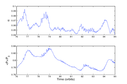
Figure 7: Plots of the turbulent stress, quantified by $\alpha$, versus time and the volume averaged pressure versus time. Parameters correspond to Set 1; there is a net toroidal-flux associated with initial $\beta=100$, and $\Sigma=250$ (UB) (see Table 1). It is clear that the latter tracks the stress imperfectly, with much of the short time scale stochastic variability seen in the stress washed out. Gross features are also associated with a time-lag of about an orbit.

This poor correlation between the viscous stress and pressure on short times casts doubt on the existence of thermal instabilities that rely on these two quantities to be functionally dependent (Shakura & Sunyaev 1976, Abramowicz et al. 1988). Indeed, numerical simulations of the MRI in radiation pressure dominated discs reveal no thermal instability (Hirose et al. 2009). Recently, linear stability analyses have been conducted that allow the pressure to lag behind stress, and vice-versa. These show that, despite this impediment, instability can in fact persist, especially with the short time-lags witnessed in our simulations (Lin et al. 2011; Ciesielski et al. 2012). It would appear then that the main obstacle to instability in turbulent models of discs is due to something else, perhaps the stochastic nature of the viscous stress which is not faithfully reproduced in the behaviour of the volume averaged pressure (Janiuk and Misra 2012).

Finally, note that over long times the turbulent stress $T_{xy}$ and pressure are correlated. Thus turbulent accretion on the hot upper branch of equilibria is greater than accretion in the colder states (cf. Section 5.1).

5.4 Numerical convergence

Finally, we briefly discuss issues associated with the numerics. Parameter set 1 was primarily undertaken with ZEUS and parameter set 2 with NIRVANA, however the two codes were run on an overlap set of some 8 simulations. The comparison yielded good agreement in both $\langle T\rangle$ and $\alpha$, with discrepancies within the range of the fluctuations. It follows that not only are our qualitative results robust with respect to parameter choices and magnetic configurations, they are robust with respect to numerical method.

In addition, we performed a short study in order to confirm that the simulations were adequately converged with respect to resolution and Reynolds number. A representative sample of runs were taken and we evaluated the quantities $\alpha$ and $\langle T\rangle$ for different Reynolds numbers while keeping the Prandtl number constant and equal to 4. In summary we found that doubling the kinematic viscosity $\nu$ (halving the Reynolds number) led to changes in $\alpha$ and $\langle T\rangle$ that were less than $5\%$. This reproduces the very weak Reynolds number dependence uncovered by Fromang (2010). Moreover, the result held whether we took 64 grid points per $H_{0}$ or 128 points. Thus we were assured that these quantities were satisfactorily converged.

Next we kept the diffusion coefficients fixed and varied the resolution. We evaluated the above quantities at both 64 and 128 grid cells per $H_{0}$. The lower resolution runs yielded slightly lower $\langle T\rangle$ but the discrepancy was within $10\%$. This small decline is understandable because at coarser resolutions more of the turbulent energy is removed by the grid and thus less captured by physical Ohmic and viscous heating. As a consequence, there is slightly less direct heating. That said, the effect is small and in general no greater than the statistical fluctuations of the runs. It leads in no way to any change in the qualitative behaviour exhibited.

Parameter Set 1: Thermal runaways
B Configuration	$\Sigma$	initial $T$	final $T$	Orbits
Zero Vertical (c)	300	$3.7\times 10^{4}$	$6.0\times 10^{3}$	60
	400	$4.0\times 10^{4}$	$3.5\times 10^{3}$	125
	500	$4.75\times 10^{4}$	$2.7\times 10^{3}$	178
Zero Vertical (h)	1700	$4.5\times 10^{3}$	$3.4\times 10^{4}$	535
Net Vertical (c)	150	$4.8\times 10^{4}$	$6.3\times 10^{3}$	20
	175	$6.5\times 10^{4}$	$7.1\times 10^{3}$	31
	188	$6.0\times 10^{4}$	$7.8\times 10^{3}$	52
Net Vertical (h)	600	$3.3\times 10^{3}$	$1.1\times 10^{4}$	101
	650	$3.3\times 10^{3}$	$1.4\times 10^{4}$	108
Net Toroidal (c)	100	$5.0\times 10^{4}$	$9.0\times 10^{3}$	14
Net Toroidal (h)	560	$3.6\times 10^{3}$	$2.5\times 10^{4}$	43
	625	$3.6\times 10^{3}$	$4.1\times 10^{4}$	73
	750	$3.0\times 10^{3}$	$4.4\times 10^{4}$	68

Table 3: Summary of the inputs and range of values found for simulations undertaken ZEUS adopting parameter set 1: $\mu=1$, $E=3.5$, $\lambda=5$. The magnetic field configuration is varied as is the input surface density $\Sigma$. These simulations resulted in thermal runaways, i.e. persistent heating or cooling as indicated by either (h) or (c) . This is because they were initially located near the corners of $S$ curves in the surface density time averaged mean temperature plane. In the latter case this occured on a time scale of a few orbits in some simulations. In general very large changes to the mean temperature in these simulations eventually resulted in the computational box becoming mismatched to the putative scale height. Accordingly, they were then not continued.

Parameter Set 2: Thermal runaways
B Configuration	$\Sigma$	initial $T$	final $T$	Orbits
Zero Vertical (c)	100	$3.18\times 10^{4}$	$3.18\times 10^{3}$	5.6
	186	$3.18\times 10^{4}$	$3.19\times 10^{3}$	17
Zero Vertical (h)	686	$8.49\times 10^{3}$	$1.70\times 10^{4}$	270
	850	$6.34\times 10^{3}$	$1.78\times 10^{4}$	155
	950	$4.75\times 10^{3}$	$1.50\times 10^{4}$	54
	1000	$6.37\times 10^{3}$	$4.07\times 10^{4}$	119
	1100	$2.00\times 10^{3}$	$1.17\times 10^{4}$	92
	1200	$6.00\times 10^{3}$	$3.18\times 10^{4}$	254
	1200	$8.00\times 10^{3}$	$5.92\times 10^{4}$	215
Net Vertical (c)	80	$3.82\times 10^{4}$	$6.37\times 10^{3}$	3.8
	100	$3.18\times 10^{4}$	$5.31\times 10^{3}$	5.25
Net Vertical (h)	275	$2.00\times 10^{3}$	$1.62\times 10^{4}$	81
	300	$1.27\times 10^{4}$	$1.78\times 10^{4}$	33
Net Toroidal (c)	80	$3.82\times 10^{4}$	$1.59\times 10^{4}$	5.9
Net Toroidal (h)	225	$4.00\times 10^{3}$	$5.56\times 10^{4}$	66
	250	$9.55\times 10^{3}$	$1.46\times 10^{4}$	43

Table 4: As in table 3 but for simulations undertaken by NIRVANA and ZEUS adopting parameter set 2: $\mu=0.5$, $E=5.66$, $\lambda=1$.

6 Conclusion

In this paper we performed a suite of numerical simulations of the MRI in local geometry with the ZEUS and NIRVANA codes. Both viscous and Ohmic heating is included, while the radiative cooling is approximated by a physically motivated cooling function that summarises the strong effect of temperature on the ability of the disc gas to retain heat. Different magnetic configurations (zero flux, net-toroidal flux, net-vertical flux) and parameters were trialed, with little change in the qualitative results.

Our simulations unambiguously exhibit the development of thermal instability and hysteresis. In particular, through a sequence of runs we can sketch out characteristic S-curves in the phase space of $(\Sigma,T_{c})$ and $(\Sigma,\dot{M})$, which are central to the classical outburst model. It hence appears that MRI turbulence is not so intermittent as to endanger the robustness of the cycle. Temperature fluctuations are well-behaved and relatively small and there is no spontaneous jumping from one stable branch to the other. Only near the ‘corners’ of the S-curve does significant stochasticity enter, as then the existence or not of a local equilibrium is uncertain. This feature will add some degree of low level ‘noise’ to the observed outburst time-series. In addition, the $\alpha$ we record on the two stable branches differ slightly but systematically. Because of the constraints of our local model, this result is more suggestive than anything else. However, it does indicate that in global disc simulations we may indeed see a systematic difference in the two branches, as required by the classical theory.

Finally, on the orbital time the turbulent stresses and pressure only weakly depend on each other in our simulations. Pressure always lags behind the turbulent stress, and thus the causality is from the stress to the pressure, via the turbulent heating (in agreement with Hirose et al. 2009). Moreover, the pressure response is a significantly ‘smoothed out’ echo of the turbulent stress features. Both facts indicate that thermal instability driven by turbulent heating variations, in which the stress is a function of pressure, may not operate in real discs. On long times, however, there is necessarily a feedback of the pressure on the stress, which leads to different accretion rates on the two branches of the S-curve.

Our work presents a first step towards unifying simulations of full MHD turbulence with the correct thermal and radiative physics of outbursting DNe and LMXBs, and possibly young stellar objects. We have begun with with the most basic model that yields the correct physics: local simulations of gas inhabiting a single radius in the disc with a simple radiative prescription. This is a ‘ground zero’ test of the compatibility of the MRI with the putative thermal limit cycles of outbursting discs. If MRI-turbulence had failed in this basic setting it would probably fail in more advanced models as well. Now that we are assured of this compatability, a variety of further work may be attempted. For instance, simulations could be performed in vertically stratified shearing boxes with more realistic radiation physics (in the flux-limited diffusion approximation with appropriate opacities). In addition, cylindrical MRI simulations should be performed with the FLP83 cooling prescription, anologous to the global $\alpha$ disc calculation of Papaloizou et al. (1983). Such simulations would describe how real turbulence mediates the heating and cooling fronts that propagate through the disc during a transition between branches.

Appendix A Radiative cooling model

In this appendix we detail how the cooling prescription of Section 3.2 was derived. In particular we show how the effective temperature $T_{e}$ is calculated within each of the three important gas regimes introduced.

A.1 Regime 1: the optically thick hot regime

The radiative cooling function can be written as a flux in the diffusion approximation by $\Lambda=\nabla\cdot\mbox{\boldmath{$F$}}$ where

$$\mbox{\boldmath{$F$}}=-\frac{4acT^{3}}{3\kappa\rho}\nabla T,$$ (24)

in which $\kappa$ is the opacity, $a=4\sigma/c$ is the Stefan-Boltzmann radiation constant and $c$ is the speed of light. Setting the optical depth as

$$\tau=\int^{\infty}_{z}\kappa(x,y,z^{\prime})\rho(x,y,z^{\prime})dz^{\prime},$$ (25)

we obtain the vertical component of $F$ in the form

$$F_{z}=\frac{4acT^{3}}{3}\frac{\partial T}{\partial\tau}.$$ (26)

We integrate from near the disc surface where $T=T_{e},$ (the effective temperature), and $\tau=\tau_{e}\sim 1$ to the mid plane where $z=0$, $T=T_{c}$ and $\tau=\tau_{c}.$ Thus we obtain

$$T^{4}_{c}-T_{e}^{4}=\int^{\tau_{c}}_{\tau_{e}}\frac{3F_{z}}{ac}d\tau,$$ (27)

where $T_{c}$ is the mid plane temperature.

In the hot optically thick Regime 1, $\tau_{c}\gg\tau_{e}\sim 1$ and $T^{4}_{c}\gg T_{e}^{4}$ so that (27) implies

$$T^{4}_{c}\sim\int^{\tau_{c}}_{1}\frac{3F_{z}}{ac}d\tau\sim\frac{3\tau_{c}}{4}T_{e}^{4},$$ (28)

where we have approximated $F_{z}$ to be constant and equal to its surface value $acT_{e}^{4}/4.$ This equation relates the effective temperature $T_{e}$ to the central temperature $T_{c}$.

To complete the prescription we take the scale height to be

$$H=({\cal{R}}T_{c}/\mu)^{1/2}\Omega^{-1},$$ (29)

and set the surface density to

$$\Sigma=2\rho_{c}H.$$ (30)

Finally, as most of the optical depth arises from the regions near the midplane, we approximate Eq. (25) by

$$\tau_{c}=\kappa_{c}\Sigma/2,$$ (31)

where $\kappa_{c}$ is the opacity evaluated at the density $\rho_{c}$ and the midplane temperature $T_{c}.$ In this hot ionised regime, we can approximate $\kappa$ by the following formula:

$$\kappa=1.5\times 10^{20}\rho T^{-2.5},$$ (32)

(FLP83). So for specified $\Omega$, the above relationships enable $T_{e}$ (and hence $\Lambda$) to be related to conditions in the mid plane, and hence $T_{c}$ and $\Sigma$.

A.2 Regime 2: the warm transitional regime

This regime exhibits a cooler disc midplane that is still well ionised but surface layers that are $\lesssim 5000$ K, and which are poorly ionised. As a result, near the photosphere $\kappa$ not only drops significantly but becomes a steeply increasing function of temperature. It follows that the requirement $\tau\sim 1$ at the photosphere determines the thermal structure of the disc, as in cool stars (Hayashi & Hoshi 1961). Instead of (28) one must impose the condition $\tau_{e}\approx 1$, where $\tau_{e}$ is the optical depth at the location where $T=T_{e}$. As the optical surface is $\sim H$ above the mid plane, it converts to a relationship between the disc surface density $T_{e}$ and $T_{c}$ that leads to the central unstable part of the S-curve when thermal equilibria are considered.

We introduce the quantity $\tau_{e}^{*}$ which we define through $\tau_{e}^{*}=\kappa_{e}\Sigma$ with $\kappa_{e}$ being the opacity evaluated at the central density $\rho_{c}$ but with the photospheric temperature $T_{e}$. It is anticipated that $\tau_{e}^{*}$ overestimates the optical depth of material above the disc photosphere $\tau_{e}$ by some factor of order unity. This factor we quantify through the dimensionless constant $E$, so that

$$E\,\tau_{e}^{*}=\tau_{e}\approx 1$$ (33)

Once the dependence of $\kappa_{e}$ on $T_{e}$ and $\rho_{c}$ is specified, equation (33) supplies a means to obtain $T_{e}$, and hence $\Lambda$, when the disc is in Regime 2. Finally, an approximate functional form of $\kappa$ in this regime of incomplete hydrogen ionisation is

$$\kappa=10^{-36}\rho^{1/3}T^{10},$$ (34)

(FLP83).

A.3 Regime 3: the cool optically thin regime

In this regime the vertical structure of the disc is isothermal with $T\approx T_{c}$. However, because the disc is optically thin in the vertical direction, $F_{z}$ is reduced from $acT_{c}^{4}/4$ by a factor $\sim 2\tau_{c}.$ Thus we set

$$T_{e}^{4}=2\lambda\tau_{c}T_{c}^{4},$$ (35)

where $\lambda$ is a dimensionless constant of order unity that takes account of appropriate frequency averaging and any other necessary corrections arising from a more complete discussion of radiation transport. This condition also connects $T_{e}$ to $T_{c}$ and $\Sigma$. The central optical depth in this regime $\tau_{c}$ is computed using Eq. (31) and the opacity prescription introduced in Eq. (34).

A.4 Interpolated form

The prescription for $T_{e}$ is given in Eq. (11) for each of the three regimes. In numerical simulations one could switch from one form to the other according to the local value of $T_{c}$; we however employ an analytic interpolation of the three forms, as in FLP83. In Eq. (11), the effective temperature $T_{e}$ takes one of three forms, which we denote by either $T_{1},\,T_{2}$ or $T_{3}$ where the subscript indicates the associated regime. These three functions are then interpolated via the following:

$$T_{e}^{4} = \frac{(T_{1}^{4}+T_{2}^{4})T_{3}^{4}}{\left[(T_{1}^{4}+T_{2}^{4})^{1/2}+T_{3}^{2}\right]^{2}},$$ (36)

(FLP83). It is this algebraic expression for $T_{e}$ that is used in Equation (10) to evaluate $\Lambda$. The two free parameters $\lambda$ and $E$ can be chosen to fit results obtained from vertical integrations with standard local $\alpha$ modelling. In Fig. (A1) we plot the resulting functional dependence of $T_{e}$ on the central temperature $T_{c}$ with the three regimes indicated on the curve. In regimes 1 and 3 the effective temperature increases steeply with central temperature, while in the transitional regime 2 the dependence is very weak on account of the rapid changes in opacity near the surface. In this intermediate regime the radiative cooling rate is very ‘flat’ and, consequently, thermal instability ensues (cf. Eq. (2)).

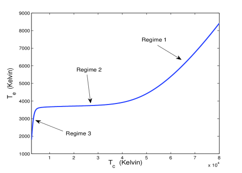
Figure 8: The effective temperature $T_{e}$ as a function of central temperature $T_{c}$ as determined from the FLP83 cooling prescription, cf. Eq. (11). Parameters are $\mu=1$, $E=3.5$ and $\lambda=5$. In addition, we have indicated on the curve which regime is dominant.

References

- (1) Abramowicz, M. A., Czerny, B., Lasota, J. P., Szuszkiewicz, E., 1988. ApJ, 332, 646.
- (2) Armitage, P. J., Livio, M., Pringle, J. E., 2002. MNRAS, 324, 705.
- (3) Balbus, S. A., Hawley, J. F., 1992. ApJ, 400, 610.
- (4) Balbus, S. A., Hawley, J. F., 1998. RvMP, 70, 1.
- (5) Balbus, S. A., Papaloizou, J. C. B., 1999. ApJ, 521, 650.
- (6) Bell, K. R., Lin, D. N. C., 1994. ApJ, 427,987.
- (7) Ciesielski, A., Wielgus, M., Kluzniak, W., Sadowski, A., Abramowicz, M., Lasota, J.-P., Rebusco, P., 2012. AA, 538, 148.
- (8) Faulkner, J., Lin, D. N. C., Papaloizou, J., 1983. MNRAS, 205, 359.
- (9) Ferreira, B. T., Ogilvie, G. I., 2009. MNRAS, 392, 428.
- (10) Fromang, S., 2010. AA, 514, L5.
- (11) Fromang, S., Papaloizou, J., Lesur, G., Heinemann, T., 2007. AA, 476, 1123.
- (12) Gallagher, J. S., Starrfield, S., 1978. AA, 12 171.
- (13) Gammie, C. F., 1996. ApJ, 553, 174.
- (14) Goldreich, P., Lynden-Bell, D., 1965. MNRAS, 130, 125.
- (15) Hawley, J. F., 2000. ApJ, 528, 462.
- (16) Hawley, J. F., Gammie, C. F., Balbus, S. A., 1995. ApJ, 440, 742.
- (17) Hayashi, C., Hoshi, R., 1961. PASJ, 13, 450.
- (18) Hirose, S., Krolik, J. H., Blaes, O., 2009. ApJ, 691, 16.
- (19) Hoshi, R., 1979. Prog. Theor. Phys. 61, 1307.
- (20) Ichikawa, S., Osaki, Y., 1992. PASJ, 44, 15.
- (21) Janiuk, A., Misra, R., 2012. AA accepted, (arXiv:1203.0139).
- (22) Kato, S, 2003. PASJ, 55, 801.
- (23) Lasota, J.-P., 2001. New Astr. Rev. 45, 449.
- (24) Lasota, J.-P., 2012. In: Eds Giovannelli, F., Sabau-Graziati, L., The Golden Age of Cataclysmic Variables and Related Objects, in press (arXiv:1111.0209)
- (25) Latter, H. N., Lesaffre, P., Balbus, S. A., 2009. MNRAS, 394, 715.
- (26) Lesaffre, P., Balbus, S. A., 2007. MNRAS, 381, 319.
- (27) Lesaffre, P., Balbus, S. A., Latter, H. N., 2009. MNRAS, 396, 779.
- (28) Lightman, A. P., Eardley, D. M., 1974. ApJ, 187, L1.
- (29) Lin, D.-B, Gu, W.-M., Lu, J.-F., 2011. MNRAS, 415, 2319.
- (30) McClintock, J. E., Remillard, R. A., 2006. In: Eds Lewin, W., van der Klis, M., Compact stellar X-ray sources, Cambridge Astrophysics Series, No. 39. Cambridge Uni. Press, Cambridge UK.
- (31) Menou, K., Hameury, J.-M, Stehle, R., 1999. MNRAS, 305, 79.
- (32) Meyer, F., Meyer-Hofmeister, E., 1981. A&A, 104, L10
- (33) Meyer, F., Meyer-Hofmeister, E., 1984. A&A, 132, 143
- (34) Papaloizou, J.C.B., Nelson, R.P., 2003. MNRAS, 339, 983.
- (35) Osaki, Y., 1974. PASJ, 26, 429.
- (36) Osaki, Y., 1994. PASJ, 26, 429.
- (37) Papaloizou, J., Faulkner, J., Lin, D. N. C., 1983. MNRAS, 205, 487.
- (38) Papaloizou, J. C. B., Pringle, J. E., 1984. MNRAS, 208, 721.
- (39) Pearson, B. R., Yousef, T. A., Haugen, N. E. L., Brandenburg, A., Krogstad, P.-A., 2004. PhRvE, 70, 6301.
- (40) Pringle, J. E., 1981. ARAA, 19, 137.
- (41) Sano, T., Inutsuka, S., 2001. ApJ, 561, L179.
- (42) Shara, M. M., 1989. PASP, 101, 5.
- (43) Shakura, N., I., Sunyaev, R. A., 1973. AA, 24, 337.
- (44) Shakura, N., I., Sunyaev, R. A., 1976. MNRAS, 175, 613.
- (45) Silvers, L. J., 2008. MNRAS, 385, 1036.
- (46) Smak, J., 1971. AcA, 21, 15.
- (47) Smak, J., 1984a. AcA, 34, 161.
- (48) Smak, J., 1984b. PASJ, 96, 5.
- (49) Starrfield, S., Sparks, W. M., Truran, J. W., Wiescher, M. C., 2000, ApJS, 127, 485.
- (50) Stone, J. M., Norman, M., L., 1992a. ApJS, 80, 753.
- (51) Stone, J. M., Norman, M., L., 1992b. ApJS, 80, 791.
- (52) Stone, J. M., Hawley, J. F., Gammie, C. F., Balbus, S. A., 1996. ApJ, 463, 656.
- (53) Warner, B., 1995. Cataclysmic variable stars. Cambridge Uni Press, Cambridge UK.
- (54) Zhu, Z, Hartmann, L., Gammie, C., McKinney, J. C., 2009. ApJ, 701, 62.
- (55) Zhu, Z., Hartmann, L., Gammie, C. F., Book, L. G., Simon, J. B., Engelhard, E., 2010. ApJ, 713, 1134.
- (56) Ziegler, U., 1999. CoPhC, 116, 65.