Planck intermediate results

We make use of the Planck all-sky survey to derive number counts and spectral indices of extragalactic sources – infrared and radio sources – from the Planck Early Release Compact Source Catalogue (ERCSC) at 100 to 857 GHz (3 mm to 350 $\mu$m). Three zones (deep, medium and shallow) of approximately homogeneous coverage are used to permit a clean and controlled correction for incompleteness, which was explicitly not done for the ERCSC, as it was aimed at providing lists of sources to be followed up. Our sample, prior to the 80 % completeness cut, contains between 217 sources at 100 GHz and 1058 sources at 857 GHz over about 12,800 to 16,550 deg² (31 to 40 % of the sky). After the 80 % completeness cut, between 122 and 452 and sources remain, with flux densities above 0.3 and 1.9 Jy at 100 and 857 GHz. The sample so defined can be used for statistical analysis. Using the multi-frequency coverage of the Planck High Frequency Instrument, all the sources have been classified as either dust-dominated (infrared galaxies) or synchrotron-dominated (radio galaxies) on the basis of their spectral energy distributions (SED). Our sample is thus complete, flux-limited and color-selected to differentiate between the two populations. We find an approximately equal number of synchrotron and dusty sources between 217 and 353 GHz; at 353 GHz or higher (or 217 GHz and lower) frequencies, the number is dominated by dusty (synchrotron) sources, as expected. For most of the sources, the spectral indices are also derived. We provide for the first time counts of bright sources from 353 to 857 GHz and the contributions from dusty and synchrotron sources at all HFI frequencies in the key spectral range where these spectra are crossing. The observed counts are in the Euclidean regime. The number counts are compared to previously published data (from earlier Planck results, Herschel, BLAST, SCUBA, LABOCA, SPT, and ACT) and models taking into account both radio or infrared galaxies, and covering a large range of flux densities. We derive the multi-frequency Euclidean level – the plateau in the normalised differential counts at high flux-density – and compare it to WMAP, Spitzer and IRAS results. The submillimetre number counts are not well reproduced by current evolution models of dusty galaxies, whereas the millimetre part appears reasonably well fitted by the most recent model for synchrotron-dominated sources. Finally we provide estimates of the local luminosity density of dusty galaxies, providing the first such measurements at 545 and 857 GHz.

1 Introduction

Figure 1: Comparison between our Planck 857 GHz mask (red indicates regions removed from the analysis) and the WMAP 7-year KQ75 mask (green means removed); unlike the case for the mask employed in this paper, the WMAP mask excludes some point sources. The background (blue) is the sky area used for our analysis. This map is a Mollweide projection of the sky in Galactic coordinates.

Among other advantages, all-sky multifrequency surveys have the benefit of probing rare and/or bright objects in the sky. One reason to probe bright objects is to study the number counts of extragalactic sources and their spectral shapes. In the far-infrared (FIR) the sources detected by these surveys are usually dominated by low-redshift galaxies with $z<0.1$, as found by IRAS at 60 $\mu$m (Ashby et al., 1996) but a few extreme objects like the lensed F10214 source (Rowan-Robinson et al., 1991) also appear. However, the population in the radio band is dominated by synchrotron sources (in particular, blazars) at higher redshift (see de Zotti et al., 2010, for a recent review). Previous multifrequency all-sky surveys were carried out in the infrared (IR) range by the IRAS satellite (between 12 and 100 $\mu$m; Neugebauer et al. 1984), and more recently by Akari (between 2 and 180 $\mu$m; Murakami et al. 2007) and WISE (between 3.4 and 22 $\mu$m; Wright et al. 2010). Early, limited sensitivity surveys were carried out in the IR and microwave range by COBE (between 1.2 $\mu$m and 1 cm; Boggess et al. 1992), and more recently in the microwave range by WMAP (between 23 and 94 GHz; Bennett et al. 2003; Wright et al. 2009; Massardi et al. 2009; de Zotti et al. 2010).

Planck’s all-sky, multifrequency surveys offer several advantages to all of the above. The frequency range covered is wide, extending from 30 to 857 GHz; observations at all frequencies were made simultaneously, reducing the influence of source variability; the calibration is uniform; and the delivered catalogue of sources used in this paper was carefully constructed and validated.

Figure 2: Comparison between our Planck 353 GHz mask (red means removed) and WMAP 7-year KQ85 mask (green). The background (blue) is the sky area used for the analysis.

Figure 3: Cumulative distribution of Planck hit counts on the sky (here at 857 GHz with Nside=2048), with the corresponding integration time per sky pixel (given on the top axis). The three sky zones used in the analysis are defined at 857 GHz: shallow (50 to 75 % of the hit count distribution, short-spaced lines, blue); medium (75 to 95 % of the hit counts, medium-spaced lines, green); and deep (95 % and above hits, widely-spaced lines, red).

The Planck frequency range fully covers the transition between the dust emission dominated regime (tracing star formation), and the synchrotron regime (tracing active galactic nuclei). The statistical analysis of the populations in this spectral range has never been done before. At large flux densities (typically 1 Jy and above), number counts from all-sky surveys of extragalactic FIR sources show a Euclidean component, i.e. a distribution of the number of source per flux density bin $S_{\nu}$ at observed frequency $\nu$ ($dN/dS_{\nu}$ in Jy^-1 sr^-1) proportional to $S_{\nu}^{-2.5}$ (see Eq.  1). This result is in line with expectations from a local Universe uniformly filled with non-evolving galaxies (Lonsdale & Hacking, 1989; Hacking & Soifer, 1991; Bertin & Dennefeld, 1997; Massardi et al., 2009; Wright et al., 2009). In the radio range, the Euclidean part is modified by the presence of higher-redshift sources. At flux densities smaller than typically 0.1 to 1 Jy, an excess in the number counts compared to the Euclidean level is an indication of evolution in luminosity and/or density of the galaxy populations. This effect is clearly seen in deeper surveys in the FIR (e.g. Genzel & Cesarsky 2000; Dole et al. 2001, 2004; Frayer et al. 2006; Soifer et al. 2008; Bethermin et al. 2010a); in the submillimetre (submm) range (e.g. Barger et al. 1999; Blain et al. 1999; Ivison et al. 2000; Greve et al. 2004; Coppin et al. 2006; Weiss et al. 2009; Patanchon et al. 2009; Clements et al. 2010; Lapi et al. 2011); – and in the millimetre and radio ranges (e.g. de Zotti et al. 2010; Vieira et al. 2010; Vernstrom et al. 2011).

Figure 4: The three sky zones used in the analysis at 857 GHz: deep (red); medium (green); and shallow (blue); These are based on the 857 GHz hit counts.

The Planck all-sky survey covers nine bands between 30 and 857 GHz. It gives us for the first time robust extragalactic counts over a wide area of sky at these wavelengths, and the first all-sky coverage between 3 mm (WMAP) and 160 $\mu$m (Akari) – e.g. see Table 1 of Planck Collaboration VII (2011). The counts in turn give us powerful constraints on the long-wavelength spectral energy distribution (SED) of the dusty galaxies investigated e.g. by IRAS, and on the short-wavelength SED of the active galaxies studied at radio wavelengths, e.g. by WMAP or ground-based facilities.

For Planck’s six highest frequency bands (100 to 857 GHz, we present here the extragalactic number counts and spectral indices of galaxies selected at high Galactic latitude and using identifications. Planck number counts and spectral indices of extragalactic radio-selected sources were already published for the frequency range 30 to 217 GHz using results from the LFI and HFI instruments (Planck Collaboration XIII, 2011). The transition between synchrotron-dominated sources and thermal dust-dominated occurs in the crucial spectral range 200-800 GHz . Thus our broader frequency data allow a better spectral characterisation of sources.

We use the WMAP 7 year best-fit $\Lambda$CDM cosmology (Larson et al., 2011), with $H_{0}$ = 71  km s^-1 Mpc^-1, $\Omega_{\Lambda}$ = 0.734 and $\Omega_{\rm M}$ = 0.266.

Figure 5: The three sky zones used in the analysis at 100 GHz: deep (red); medium (green); and shallow (blue). These are based on the 100 GHz hit counts.

Figure 6: Completeness (vs. flux density of sources) coming from the Monte-Carlo runs for the ERCSC and derived for each zone. The horizontal dashed line represents our threshold for number count analysis.

2 Planck data, masks and sources

Planck (Tauber et al., 2010; Planck Collaboration I, 2011) is the third generation space mission to measure the anisotropy of the cosmic microwave background (CMB). It observes the sky in nine frequency bands covering 30–857 GHz with high sensitivity and angular resolution from 31^′ to 5^′. The Low Frequency Instrument LFI; (Mandolesi et al., 2010; Bersanelli et al., 2010; Mennella et al., 2011) covers the 30, 44, and 70 GHz bands with amplifiers cooled to 20 K. The High Frequency Instrument (HFI; Lamarre et al. 2010; Planck HFI Core Team 2011a) covers the 100, 143, 217, 353, 545, and 857 GHz bands with bolometers cooled to 0.1 K. Polarization is measured in all but the highest two bands (Leahy et al., 2010; Rosset et al., 2010). A combination of radiative cooling and three mechanical coolers produces the temperatures needed for the detectors and optics (Planck Collaboration II, 2011). Two Data Processing Centers (DPCs) check and calibrate the data and make maps of the sky (Planck HFI Core Team, 2011b; Zacchei et al., 2011). Planck’s sensitivity, angular resolution, and frequency coverage make it a powerful instrument for galactic and extragalactic astrophysics as well as cosmology. Early astrophysics results are given in Planck Collaboration VIII–XXVI 2011, based on data taken between 13 August 2009 and 7 June 2010. Intermediate astrophysics results are now being presented in a series of papers based on data taken between 13 August 2009 and 27 November 2010.

The Planck data used in this paper (unlike other intermediate Planck papers) come entirely from the Early Release Compact Source Catalogue, or ERCSC (Planck Collaboration VII, 2011; Planck Collaboration, 2011). This in turn is based on Planck’s first 1.6 sky surveys, data taken between 13 August 2009 and 7 June 2010. First results from the ERCSC are published as Planck early papers (Planck Collaboration XIII, 2011; Planck Collaboration XIV, 2011; Planck Collaboration XV, 2011; Planck Collaboration XVI, 2011). In this paper, we use only HFI data, covering the 100–857 GHz range in six bands.

2.1 Galactic masks

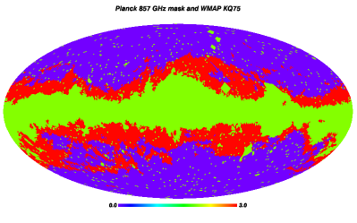
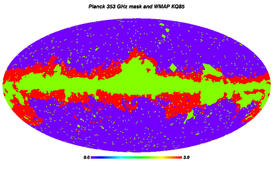
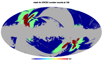
To obtain reliable extragalactic number counts, uncontaminated by Galactic sources, we mask out areas of the sky strongly affected by Galactic sources, defining a set of “Galactic masks”. These are based on removing a fraction of the sky above a specified level in sky surface brightness. We use two masks, one at high frequencies (857 and 545 GHz), and one at lower frequencies (353 GHz and below). The use of two different masks is motivated by the different astrophysical components dominating the higher HFI frequencies and the lower frequencies, which are not necessarily spatially correlated. While emission from Galactic dust dominates at 857  GHz, its spectrum decreases with decreasing frequency. On the contrary, the synchrotron and free-free components dominate at 100 GHz.

Before applying a brightness cut to the maps, we degrade the angular resolution of the maps from 1.^′5 ($N_{\rm side}$=2048 in Healpix; Górski et al. 2005) down to 55^′($N_{\rm side}$=64). The maps at low resolution are then interpolated at the original high angular resolution. Creating a Galactic mask using this procedure has the double benefit of: 1) not masking the bright sources (because they are smoothed away); and 2) smoothing the Galactic structure. We checked to make sure that even the brightest sources remained unmasked after applying this smoothing.

The 857 GHz Galactic mask keeps 48 % of the sky for analysis (thus removing 52 % of the sky), and this corresponds to a cut of 2.2 MJy sr^-1 at 857 GHz. This mask is applied at 857 and 545 GHz. The 353 GHz Galactic mask keeps 64 % of the sky for analysis (thus removing 36 % of the sky), and corresponds to a cut of 0.28 MJy sr^-1 at 353 GHz.This mask is applied at 353, 217, 143 and 100 GHz.

Figs. 1 and 2 show the Planck masks, comparing them with the WMAP 7 year KQ75 and KQ85 masks (Gold et al., 2011; Jarosik et al., 2011). Note that we do not use the WMAP masks in this work.

2.2 Three zones in the sky: deep, medium and shallow

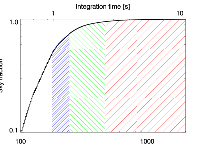
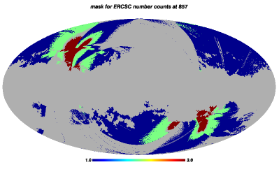
Three main zones are identified to ensure reasonably homogeneous coverage of the sky by the Planck detectors at each frequency, thereby allowing a clean and simple estimate of the completeness. As noted above, the Planck data used here correspond to approximately 1.6 complete surveys of the sky; in addition each survey has non-uniform coverage of the sky (Planck Collaboration I, 2011; Planck HFI Core Team, 2011a, b). While performing statistics on sources drawn from a non-uniformly covered survey is feasible, both the nature of the Planck data (including scanning strategy, and masking of planets (see the ERCSC article Planck Collaboration VII 2011) and its heterogeneous coverage (see Fig. 3) make it difficult to implement. We therefore select three zones in the sky, in each of which the observations are approximatively homogeneous in integration time.

The hit count can be defined by counting the number of times a single Planck detector observes one sky position in the sky. The hit count can also be defined for a particular frequency band: it is the number of times each sky pixel has been hit by any Planck detector at a given frequency. We will be using this latter definition. This quantity is similar to $N_{\rm obs}$ in WMAP data files.

The three zones have hit counts varying by not more than a factor of two, except in the smaller deep zone (at the ecliptic poles) where there is high redundancy. They are defined as (and illustrated in Fig. 3):

• deep: $<$5% of the best covered sky fraction (or 95 % or more of the cumulative hit count distribution at a given frequency);

• medium: 5 to 25% of the best covered sky fraction (or 75 to 95 % of the cumulative hit count distribution at a given frequency);

• shallow: 25 to 50% of the best covered sky fraction (or 50 to 75 % of the cumulative hit count distribution at a given frequency).

Thus, pixels in the deep zone (at a given frequency) all have a hit count value greater than or equal to the hit count value corresponding to 95 % of the total distribution at this frequency. Note that each frequency map has different hit counts, due to the focal plane geometry; each zone will thus have slight differences in geometry from one frequency to another, leading to slightly different surface areas. Table 2 summarizes the surface area of each zone; typically, the deep zone covers 1000 deg², the medium zone about 3000 deg², and the shallow about 12000 deg². Fig. 4 (or 5) shows the three different zones used in this analysis: deep, medium and shallow at 857 GHz (100 GHz), respectively.

Table 1: Percentage and number of Planck source identifications using the SIMBAD and NED databases.

        Galactic

        Extragal         Insecure         Secure         Unident         Total

Zone         % $$N$$         %         %         %         %

857 deep.         91.2 73         2.5 2         1.2 1         5.0 4         100 80

medium.         95.5 255         1.9 5         0.0 0         2.6 7         100 267

shallow .         94.6 697         1.6 12         0.8 6         3.0 22         100 737

545 deep .         76.5 39         7.8 4         2.0 1         13.7 7         100 51

medium .         91.1 143         2.5 4         0.0 0         6.4 10         100 157

shallow .         91.8 301         2.1 7         0.9 3         5.2 17         100 328

353 deep .         81.6 31         2.6 1         5.3 2         10.5 4         100 38

medium .         87.0 94         0.9 1         2.8 3         9.3 10         100 108

shallow .         78.0 170         4.6 10         4.6 10         12.8 28         100 218

217 deep .         77.3 17         0.0 0         22.7 5         0.0 0         100 22

medium .         92.5 62         1.5 1         1.5 1         4.5 3         100 67

shallow .         88.5 170         0.5 1         4.2 8         6.8 13         100 192

143 deep .         86.7 13         0.0 0         13.3 2         0.0 0         100 15

medium .         100.0 48         0.0 0         0.0 0         0.0 0         100 48

shallow .         96.8 182         0.5 1         1.6 3         1.1 2         100 188

100 deep .         77.8 14         0.0 0         22.2 4         0.0 0         100 18

medium .         100.0 45         0.0 0         0.0 0         0.0 0         100 45

shallow .         93.9 154         0.0 0         3.7 6         2.4 4         100 164

Table 2: Number of extragalactic sources by zone before (after) the completeness cut, and the surface area of the zones.

$$\nu N$$       Before (After) Completeness Cut      Surface Area [deg²] [GHz]      Deep Medium Shallow Total      Deep Medium Shallow Total 857.      77 (24) 262 (115) 719 (313) 1058 (452)      880 2288 9800 12969 545.      46 (8) 153 (69) 318 (143) 517 (220)      874 2324 9551 12749 353.      35 (14) 104 (59) 198 (151) 337 (224)      1086 2971 12373 16431 217.      17 (15) 65 (57) 183 (71) 265 (143)      1104 3169 11900 16174 143.      13 (8) 48 (44) 184 (90) 245 (142)      1111 2972 11977 16061 100.      14 (6) 45 (39) 158 (77) 217 (122)      1072 2870 12611 16554

Table 3: Number of extragalactic sources used in the deep (D), medium (M), and shallow (S) number counts, and the corresponding number of unidentified sources.

$$N_{\rm used} N_{\rm unidentified} S_{\nu} \ldots \ldots \ldots \ldots \ldots \ldots \ldots \ldots \ldots \ldots \ldots \ldots \ldots \ldots \ldots \ldots \ldots \ldots \ldots \ldots \ldots \ldots \ldots \ldots \ldots \ldots \ldots \ldots \ldots \ldots \ldots \ldots \ldots \ldots \ldots \ldots \ldots \ldots \ldots \ldots \ldots \ldots \ldots \ldots \ldots \ldots \ldots \ldots \ldots \ldots \ldots \ldots \ldots \ldots \ldots \ldots \ldots \ldots \ldots \ldots \ldots$$/ [Jy] 857 GHz 545 GHz 353 GHz 217 GHz 143 GHz 100 GHz D M S D M S D M S D M S D M S D M S 0.398 0.303–0.480 7/0 28/1 92/9 3/0 12/0 81/1 0.631 0.480–0.762 8/0 31/4 83/14 3/0 13/1 34/2 2/0 13/0 43/0 4/0 15/0 68/3 1.000 0.762–1.207 4/0 18/2 38/7 4/0 8/0 21/1 4/0 10/0 25/0 4/0 11/0 47/1 1.585 1.207–1.913 5/0 26/6 78/9 1/1 6/0 14/0 1/0 4/0 11/0 2/0 4/0 12/0 2/0 7/0 13/0 2.512 1.913–3.032 11/0 31/1 139/4 0/0 20/1 28/1 1/0 2/0 8/0 1/0 3/0 3/0 5/0 3/0 11/0 3.981 3.032–4.805 7/0 33/2 95/4 1/0 16/1 20/1 1/0 6/0 2/0 1/0 1/0 3/0 2/0 3/0 6.310 4.805–7.615 3/0 22/2 41/7 1/0 6/0 8/1 1/0 1/0 1/0 1/0 2/0 10.000 7.615–12.069 2/0 20/1 23/1 1/0 1/0 5/0 1/0 1/0 1/0 15.849 12.069–22.801 1/0 9/0 15/0 0/0 0/0 4/0 2/0

Figure 7: Distribution of spectral indices (for the sources present in the ERCSC at a given frequency in our sample with completeness of 80 % or above). Here $\alpha^{217}_{143}$ is shown as a dotted line, $\alpha^{353}_{217}$ as a dashed line, and $\alpha^{857}_{545}$ as a solid line. The region $2\leq\alpha\leq 4$ is typical of thermal dust emission. In red we show the dusty sources, whereas in blue we show the synchrotron sources. The sources in all three samples (deep, medium, and shallow) are combined here. Note that, as expected, the 100 GHz, and 143 GHz samples are dominated by radio galaxies, whereas the 545 GHz and 857 GHz samples are dominated by dusty galaxies. At 217 GHz and 353 GHz we observe the transition between the two populations, with significant numbers of both types being present in the samples.

2.3 Sample selection and validation

The sample is drawn from the ERCSC (Planck Collaboration VII, 2011), which was constructed to contain high SNR sources. Notice that at high frequency, the noise is dominated by the confusion, mainly due to faint extragalactic sources and Galactic cirrus (Condon, 1974; Hacking et al., 1987; Franceschini et al., 1989; Helou & Beichman, 1990; Franceschini et al., 1991, 1994; Toffolatti et al., 1998; Dole et al., 2003; Negrello et al., 2004; Dole et al., 2006). The selection is performed with the following steps at each HFI frequency independently:

• select sources within each zone: deep, medium and shallow;

• select point sources, using the keyword “EXTENDED” set to zero;

These criteria should favour the presence of galaxies rather than Galactic sources. To validate this, we make three checks in addition to using conservative masks.

1. We measure the mid-IR to  submm flux density ratios of known Galactic cold cores (from the Planck Early Cold Core catalogue, ECC, Planck Collaboration XXIII 2011) and conversely of known galaxies in the ERCSC. Using WISE (Wright et al., 2010) W3 and W4 bands (when available with the first public release), and the 857 GHz HFI band, we measure a factor of 100 to 200 between the submm-to-mid-infared ratios of galaxies and ECC sources. When measuring this ratio in our sample, we see that the submm-to-mid-infared colours of all sources in our sample are compatible with galaxy colours, and not with ECC colours.

2. The CIRRUS flag in the ERCSC gives an estimate of the normalised neighbour surface density of sources at 857 GHz, as a proxy for cirrus contamination. The median value of the CIRRUS flag in our sample is 0.093 at 857 GHz, a low value compatible with no cirrus contamination when used in conjunction with the EXTENDED=0 flag (e.g. Herranz et al. 2012).

3. We query the NED and SIMBAD databases at the positions of all our ERCSC sources using a 2.^′5 search radius. Each Planck source has many matches (many of them completely unrelated, e.g. foreground stars), and the identification is more complex at higher frequencies. However, as we show later, our $N(>S)$ cumulative distribution of sources is always less than 200 sources per steradian, i.e. less than $3.3\times 10^{-4}$ ERCSC sources per 2.^′5 search radius on average. We thus search for the most probable match by identifying the source type in this order: Galactic, then extragalactic. The Galactic types include supernova remnants, planetary nebulae, nebulae, Hii regions, stars, molecular clouds, globular/star clusters. We call a source “Galactic unsecure” when one of the two databases returns no identification and the other a Galactic identification. We do not use “Galactic secure” or “Galactic un-secure” sources in the analysis in this paper. The statistics of identifications is given in Table 1.

Our final sample is composed of confirmed galaxies, the vast majority being NGC, IRAS, radio galasy and blazar objects, as well as some unidentified sources (a small fraction of the total number). The few completely unidentified sources, where no SIMBAD or NED ID was found, are interpreted as potential galaxies, and hence are included in our counts, because they have a small cirrus flag value (see point 2 above). Their relatively small number don’t change the results presented in this article, wether or not we include these sources.

Table 2 summarises the source number and surface area of each zone (deep, medium and shallow). We find a total number of sources ranging from 217 at 100 GHz to 1058 at 857 GHz.

2.4 Completeness

The ERCSC Pipeline (Planck Collaboration VII, 2011) used extensive Monte-Carlo simulations ( to account for systematic and sky noise) to assess various parameters such as positional or flux density accuracies. Here, we use the results of those runs to estimate the completeness in each of the three zones, as presented in Fig. 6. The uncertainties in completeness are at the 5 % level, as discussed in Planck Collaboration VII (2011) and Planck Collaboration (2011). The correction for incompleteness is then applied to the number counts of each zone separately.

We use a completeness level threshold of 80 % for all frequencies. This ensures: 1) minimal source contamination; 2) no photometric biases (Planck Collaboration, 2011); and 3) good photometric accuracy (Planck Collaboration, 2011) – see Sect. 2.5. The number of sources actually used to estimate the number counts is given in Tab. 3, which also includes the number of unidentified sources. In the end, we use a number of sources ranging from 122 at 100 GHz to 452 at 857 GHz (Tab. 2).

Figure 8: Fraction of galaxy types as a function of frequency, on the sample having completeness of 80 % and above: dusty (red squares) and synchrotron (blue triangles). Error bars are Poissonian.

Table 4: Planck number counts at 353, 545, and 857 GHz.

      857 GHz       545 GHz       353 GHz

$$S_{\nu}$$ [Jy]                     

Mean Range       [Jy^1.5 sr^-1] [sr^-1]       [Jy^1.5 sr [sr^-1]       [Jy^1.5 sr^-1] [sr^-1]

0.631 0.480–0.762                     

1.000 0.762–1.207                     

1.585 1.207–1.913                     

2.512 1.913–3.032                     

3.981 3.032–4.805                     

6.310 4.805–7.615                     

10.000 7.615–12.069                     

15.849 12.069–22.801                     

Table 5: Planck number counts at 100, 143, and 217 GHz.

      217 GHz       143 GHz       100 GHz

$$S_{\nu}$$ [Jy]                     

Mean Range       [Jy^1.5 sr^-1] [sr^-1]       [Jy^1.5 sr [sr^-1]       [Jy^1.5 sr^-1] [sr^-1]

0.398 0.303–0.480                     

0.631 0.480–0.762                     

1.000 0.762–1.207                     

1.585 1.207–1.913                     

2.512 1.913–3.032                     

3.981 3.032–4.805                     

6.310 4.805–7.615                     

10.000 7.615–12.069                     

2.5 Photometry

The photometry of the ERCSC is extensively detailed in Planck Collaboration VII (2011) as well as in the explanatory supplement Planck Collaboration (2011). Here we use the “FLUX” field for flux densities. Notice that 100 and 217 GHz flux densities can be affected by Galactic CO lines (Planck HFI Core Team, 2011b).

We would like to emphasise that the extensive simulations performed in the process of generating/validating the ERCSC allow us to derive reliable completeness estimates for each zone (see Sect. 2.4) and also to estimate the quality of the photometry. In the faintest flux density bins that we are using (corresponding to 80 % completeness), there is no photometric offset, and the photometric accuracy from the Monte-Carlo simulations (Planck Collaboration, 2011, ; Fig. 7 for reference) is about: 35 % at 480 mJy for 100 GHz; 30 % at 300 mJy for 143 GHz; 20 % at 300 mJy for 217 GHz; 20 % at 480 mJy for 353 GHz; 20 % at 1207 mJy for 545 GHz; and 20 % at 1913 mJy for 857 GHz. This scatter in the faintest flux density bins strongly decreases at larger flux densities. Note that photometric uncertainties can bias the determination of the counts slope (e.g. Murdoch, Crawford & Jauncey, 1973); at our completeness level, the effect is negligible.

From our sample, we also create “Band-filled catalogues”. For each frequency/zone sample, we take each source position from the ERCSC and perform aperture photometry from the corresponding images in the other frequencies. We adopt 4 $\sigma$ as the detection threshold. These aperture photometry measurements (and upper limits) are used for the spectral classification of sources and in the spectral index determinations, but not in the number counts measurements (which rely only on ERCSC flux densities). We define the spectral index $\alpha$ by $S_{\nu}\propto\nu^{\alpha}$.

The derived spectral indices are used to determine the colour correction of the ERCSC flux densities (Planck HFI Core Team, 2011b). This correction changes the flux densities by at most 5 % at 857 GHz, 15 % at 545 GHz, 14 % at 353 GHz, 12 % at 217 GHz, and 1 % at 143 GHz and 100 GHz.

Table 6: Planck number counts of dusty galaxies at 217, 353, 545, and 857 GHz.

$$S_{\nu} {dN\over dS_{\nu}}S_{\nu}^{2.5} \ldots \ldots \ldots 3.2\pm 0.7 \ldots \ldots 23.6\pm\kern 4.00002pt3.1 2.3\pm 0.8 \ldots \ldots 18.5\pm\kern 4.00002pt3.2 1.8\pm 0.9 \ldots 129.0\pm 21.1 12.5\pm\kern 4.00002pt3.4 \ldots 463.6\pm\kern 4.00002pt70.2 100.3\pm 19.8 11.7\pm\kern 4.00002pt4.5 1.7\pm 1.7 609.0\pm\kern 4.00002pt\kern 4.00002pt6.0 151.5\pm 32.5 13.3\pm\kern 4.00002pt6.7 \ldots 573.4\pm 103.4 129.4\pm 37.5 \ldots \ldots 755.2\pm 150.3 119.5\pm 47.8 13.2\pm 13.3 \ldots 837.1\pm 200.5 136.2\pm 70.4 26.4\pm 26.5 \ldots$$ [Jy]        [Jy^1.5 sr^-1] Mean Range       857 GHz 545 GHz 353 GHz 217 GHz 0.398 0.303–0.480        0.631 0.480–0.762        1.000 0.762–1.207        1.585 1.207–1.913        2.512 1.913–3.032        3.981 3.032–4.805        6.310 4.805–7.615        10.000 7.615–12.069        15.849 12.069–22.801       

Table 7: Planck number counts of synchrotron galaxies at 100, 143, 217, 353, 545, and 857 GHz.

$$S_{\nu} {dN\over dS_{\nu}}S_{\nu}^{2.5} \ldots \ldots \ldots 13.3\pm 1.7 \kern 4.00002pt8.5\pm\kern 4.00002pt1.1 \ldots \ldots \ldots \kern 4.00002pt7.0\pm\kern 4.00002pt1.4 \kern 4.00002pt9.2\pm 1.6 13.5\pm\kern 4.00002pt2.1 21.9\pm\kern 4.00002pt3.0 \ldots \ldots \kern 4.00002pt7.9\pm\kern 4.00002pt2.0 12.8\pm 2.6 16.9\pm\kern 4.00002pt3.1 28.6\pm\kern 4.00002pt4.3 \ldots 2.4\pm 1.7 \kern 4.00002pt5.0\pm\kern 4.00002pt2.1 13.6\pm 3.6 15.4\pm\kern 4.00002pt3.8 18.8\pm\kern 4.00002pt4.3 2.6\pm 2.6 4.3\pm 3.1 \kern 4.00002pt6.7\pm\kern 4.00002pt3.4 \kern 4.00002pt5.1\pm 3.0 13.6\pm\kern 4.00002pt5.0 23.2\pm\kern 4.00002pt6.5 4.5\pm 4.6 8.7\pm 6.2 10.0\pm\kern 4.00002pt5.8 10.1\pm 5.9 13.6\pm\kern 4.00002pt6.9 16.5\pm\kern 4.00002pt7.5 \ldots \ldots \ldots 13.5\pm 9.6 13.6\pm\kern 4.00002pt9.7 13.2\pm\kern 4.00002pt9.4 \ldots \ldots \ldots \ldots 13.6\pm 13.6 26.3\pm 18.7 \ldots \ldots 26.4\pm 26.5 \ldots \ldots \ldots$$ [Jy]        [Jy^1.5 sr^-1] Mean Range       857 GHz 545 GHz 353 GHz 217 GHz 143 GHz 100 GHz 0.398 0.303–0.480        0.631 0.480–0.762        1.000 0.762–1.207        1.585 1.207–1.913        2.512 1.913–3.032        3.981 3.032–4.805        6.310 4.805–7.615        10.000 7.615–12.069        15.849 12.069–22.801       

3 Classification of galaxies into dusty or synchrotron categories

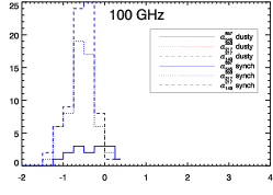
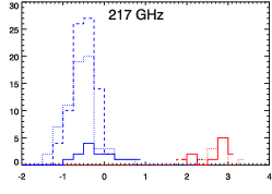
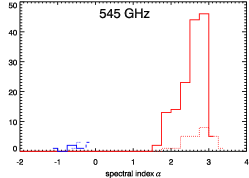
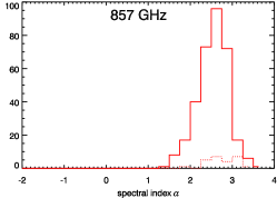
For the purposes of this paper, we aim for a basic classification based on SEDs that separates sources into those dominated by thermal dust emission and those dominated by synchrotron emission. (Free-free emission does exist, but is not dominant, e.g., Peel et al. 2011). In order to classify our sources by type, we start with the band-filled catalogues discussed in Section 2.5. Thermal dust emission is expected to show spectral indices in the range $\alpha$ $\sim$ 2 – 4. On the other hand, colder temperature sources can show lower $\alpha^{857}_{545}$, if the 857 GHz measurement falls near the spectral peak. Also, the presence of a strong synchrotron component, or perhaps a free-free emission component, would start to flatten the SED below $\sim$ 353 GHz. With such issues in mind, we have set up the following classification algorithm:

• all sources with $\alpha^{857}_{545}$ $\geq$ 2, or $\alpha^{545}_{353}$ $\geq$ 2 are assigned a “dusty” classification;

• all sources where both of these spectral indices are lower than 2, including non-detections, are assigned “synchrotron” classification.

The resulting classification is summarised in Fig. 7, showing the spectral index distributions for each type as a function of observed frequency.

However, some sources are difficult to classify, and could be part of an “intermediate dusty” or “intermediate synchrotron” type. These intermediate sources can be defined as follows:

• being dusty (according to our criterion above) but also having $\alpha^{857}_{100}<1$

• being synchrotron (according to our criterion above) but also being detected either at 857 or 545 GHz, and undetected at 353 and 217 and 143 GHz, i.e. sources that show both a significant dust component and a strong synchrotron component.

Figure 9: Planck differential number counts, normalised to the Euclidean value (i.e. $S^{2.5}dN/dS$), compared with models and other data sets. Planck counts: total (black filled circles); dusty (red circles); synchrotron (blue circles). Four models are also plotted: de Zotti et al. (2005, dealing only with synchrotron sources – solid line); Tucci et al. (2011, dealing only with synchrotron sources – dots); Bethermin et al. (2011, dealing only with dusty sources – long dashes); Serjeant & Harrison (2005, dealing only with local dusty sources – short dashes). Other data sets: Planck early counts for 30 GHz-selected radio galaxies (Planck Collaboration XIII, 2011) at 100, 143 and 217 GHz (open diamonds); Herschel ATLAS and HerMES counts at 350 and 500 $\mu$m from Oliver et al. (2010) and Clements et al. (2010); BLAST at the same two wavelengths, from Bethermin et al. (2010b); all shown as triangles. Left vertical axes are in units of Jy^1.5 sr^-1, and the right vertical axis in Jy^1.5.deg^-2.

Among the sources included in the number counts analysis, fewer than 10 % are classified as “intermediate”. This fraction rises significantly if we remove the completeness cut due to the increasing photometric uncertainties at lower flux densities (see Appendix A for details). Examples of both “dusty” or “synchrotron” sources with somewhat unusual SEDs are discussed in Appendix B .

4 Planck extragalactic number counts between 100 and 857 GHz

The Planck extragalactic number counts (differential, normalised to the Euclidean slope, and completeness-corrected) are presented in Fig. 9 and Tables 4 and 5. They are obtained using a mean of the 3 zones (weighted by the surface area of each zone).

The error budget in the number counts is made up of: (i) Poisson statistics (ii); the 5 % uncertainty in the completeness correction (iii); the absolute photometric calibration uncertainty of 2 % at and below 353 GHz, and 7 % above 545 GHz (Planck HFI Core Team, 2011a, b). According to e.g. Eq. 1 of Bethermin et al. (2011), calibration uncertainties produce errors scaling as the 1.5 power in the Euclidean, normalized, differential number counts.

Notice that for our bright counts, the error budget is dominated by sample variance of nearby sources and consequently by small-number statistics. For instance, the small wiggle seen in the counts at the three highest frequencies (seen at 600 mJy at 353 GHz, 4 Jy at 545 GHz and 10 Jy at 857 GHz) is due to a few tens of local NGC sources in the medium zone (see Appendices B and C).

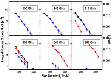
Integral (i.e. cumulative) combined number counts are shown in Fig. 11. Although error bars are highly correlated, these counts provide a useful estimate of the source surface density. The completeness correction is also applied here, and we use the same cuts in flux density as for the differential counts. Tab. 4 and 5 also give the $N>S$ values.

5 Further Results & Discussion

5.1 Nature of the Galaxies at submillimetre and millimetre wavelengths

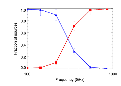
The change in the nature of sources (synchrotron dominated vs. dusty) with frequency was first observed in the Planck data in Planck Collaboration VII (2011). Our new sample allows a more precise quantification because of its completeness. The statistics of synchrotron vs. dusty galaxies are summarised in Fig. 8, showing the fraction of galaxy type as a function of frequency. We estimate the uncertainty in the classification to be of the order of 10 % (see Appendix A). The striking result is the almost equal contribution of both source types near 300 GHz. The high frequency channels (545 and 857 GHz) are, unsurprisingly, dominated ($>90\thinspace\%$) by dusty galaxies. The low frequency channels are, unsurprisingly, dominated ($>95\thinspace\%$) by synchrotron sources at 100 and 143 GHz. At 217 GHz, fewer than 10 % of the sources show a dust-dominated SED.

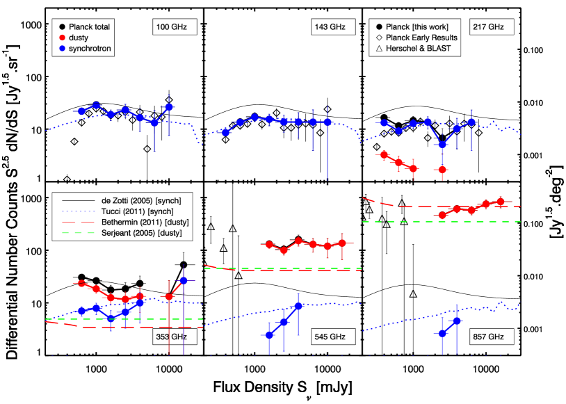
All the sources from our complete sample have an identified spectral type (by construction), and we can compute the number counts separately for synchrotron and dusty galaxies. Fig. 9, 10 and 11 show the differential and integral number counts by type, also given in Tables 6 and 7. We note that at 353 GHz, about two thirds of the number counts are made-up by dusty sources. At 217 GHz (545 GHz) there is a minor contribution (10 % or less) of the dusty (synchrotron) sources contributing to the counts. These number counts of extragalactic dusty and synchrotron sources are an important step towards further constraining models of galaxy SED and to including the results in more general models of galaxy evolution (see below).

5.2 Planck Number Counts Compared with Other Datasets

The number counts are in fairly good agreement at lower frequencies (100 to 217 GHz) with the counts published in the Planck early results, based on a 30 GHz selected sample (Planck Collaboration XIII (2011); represented as diamonds in Fig. 9 and 10). The effect of incompleteness in the latter is seen in the fainter flux density bins, below about 500 mJy. We also notice a slight disagreement around 400 mJy at 217 GHz, where our counts of synchrotron galaxies exceed the Planck early counts by a factor of 1.7 ($13.7\pm 1.5$ vs. $8.2\pm 0.9\thinspace$Jy^1.5 sr^-1). This discrepancy can be easily understood: our current selection of synchrotron sources is not the same as the one adopted in the Planck Early results paper Planck Collaboration XIII (2011), in which a more restrictive criterion was used ($\alpha^{217}_{143}<0.5$). If we adopt the same criterion as in that paper, we find no statistically significant difference between the two estimates of the number counts.

Our estimates of counts also seem consistent with the Herschel ATLAS and HerMES counts (Clements et al., 2010; Oliver et al., 2010) at high frequency (545 and 857 GHz) as well as BLAST at the same two wavelengths (Bethermin et al., 2010b), although there is no direct overlap in flux density and small number statistics affect the brightest Herschel points.

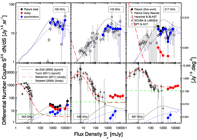
The ACT 148 GHz data (Marriage et al., 2011) and SPT 150 and 220 GHz (Vieira et al., 2010) data are also plotted in Fig. 10, together with SCUBA and LABOCA data at 353 GHz (Borys et al., 2003; Coppin et al., 2006; Scott et al., 2006; Beelen et al., 2008; Weiss et al., 2009). The ACT and SPT data, when added to the Planck data at 143 GHz, cover more than four orders of magnitude in flux density.

Finally, we checked that our counts are in agreement with the Planck Sky Model (Delabrouille et al., 2012).

Figure 10: Same as Fig. 9, but on a wider flux density scale and with the addition of ACT (Marriage et al., 2011) and SPT (Vieira et al., 2010) data shown as squares at 143 and 217 GHz, and SCUBA and LABOCA data shown as stars at 353  GHz (Borys et al., 2003; Coppin et al., 2006; Scott et al., 2006; Beelen et al., 2008; Weiss et al., 2009). Notice that we added the model of Bethermin et al. (2011) at 500 $\mu$m (dash-dot) to comply with the Herschel data taken at that wavelength (and not at 545 GHz).

Figure 11: Planck integral number counts (filled circles); dusty (red); synchrotron (blue). Vertical axes are in number per steradian; right axis is in number per square degree. Counts are completeness-corrected. The same faint flux density cut as for differential counts is applied.

Figure 12: Planck differential number counts at 857 GHz, normalised to the Euclidean (i.e. $S^{2.5}dN/dS$). Planck counts: total (black filled circles); dusty galaxies (red circles). Models: Bethermin et al. (2011) (long red dashes – dusty); Serjeant & Harrison (2005) (short green dashes – dusty); Rahmati & van Der Werf (2011) (black dash-dot-dot-dot line). Other: Lagache et al. (2004); Negrello et al. (2007); Rowan-Robinson (2009); Valiante et al. (2009); Pearson & Khan (2009); Franceschini et al. (2010); Lacey et al. (2010); Wilman et al. (2010).

5.3 Planck Number Counts and Models

5.3.1 Models

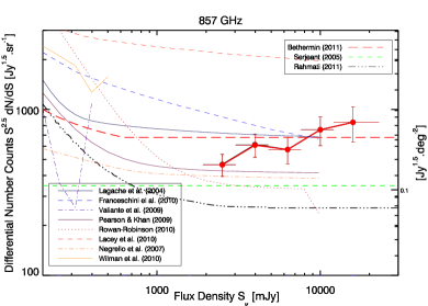
Fig. 9 and 10 display our present estimates of number counts of extragalactic point sources, based on ERCSC data, together with predictions from recent models of the numbers and evolution of extragalactic sources. These models focus either on radio-selected sources – i.e. sources with spectra dominated by synchrotron radiation at mm/submm wavelengths (“synchrotron sources”): de Zotti et al. (2005) and Tucci et al. (2011) – or on far-IR selected sources – i.e. sources with spectra dominated by thermal cold dust emission at mm/submm wavelengths (“dusty sources”): Serjeant & Harrison (2005) and Bethermin et al. (2011). Many other models exist in the literature, among which are Le Borgne et al. (2009), Negrello et al. (2007), Pearson & Khan (2009), Rowan-Robinson (2009), Valiante et al. (2009), Franceschini et al. (2010), Lacey et al. (2010), Marsden et al. (2011), Wilman et al. (2010), and Rahmati & van Der Werf (2011). A comparison is given with these models in Fig. 12 for 857 GHz.

The de Zotti et al. (2005) model focusses on radio sources, both flat- and steep-spectrum, the latter having a component of dusty spheroidals and GPS (GHz peaked spectrum) sources. It includes cosmological evolution of extragalactic radio sources, based on an analysis of all the main source populations at GHz frequencies. It currently provides a good fit to all data on number counts and on other statistics from $\sim 5\thinspace$GHz up to $\sim 100\thinspace$GHz. This model adopts a simple power-law, with a very flat spectral index ($\alpha\simeq-0.1$), for extrapolating the spectra of the brightest extragalactic sources (essentially “blazar sources”) to frequencies above 100 GHz.

The Tucci et al. (2011) models provide a description of three populations of radio sources: steep-, flat-, and inverted-spectrum. The flat-spectrum population is further divided into Flat-Spectrum Radio Quasars (FSRQ), and BL Lacs. The main novelty of these models is the statistical prediction of the “break” frequency, $\nu_{\rm M}$, in the spectra of blazar jets modeled by classical, synchrotron-emission physics. The most successful of these models, “C2Ex”, assumes different distributions of break frequencies for BL Lac objects and Flat Spectrum Radio Quasars, with the relevant synchrotron emission coming from more compact regions in the jets of the former objects. This model, developed to fit both the Atacama Cosmology Telescope (ACT) data (Marriage et al., 2011) at 148 GHz and the results published in the Planck Early paper Planck Collaboration XIII (2011), is able to give a very good fit to all published data on statistics of extragalactic radio sources: i.e. number counts and spectral index distributions. The model “C2Ex” also correctly predicts the number of blazars observed in the Herschel Astrophysical Terahertz Large Area Survey (H-ATLAS) at 600 GHz, as discussed in López-Caniego et al. (2012).

The Serjeant & Harrison (2005) model is based on the SED properties of local galaxies detected by IRAS and by SCUBA in the SLUGS sample (Dunne et al., 2000). These local SEDs are used in many models, including the Lapi et al. (2011) model (based on Lapi et al. 2006 and Granato et al. 2004) which links dark matter halo masses with the mass of black holes and the star formation rate.

Bethermin et al. (2011) present a backwards evolution model, taking into account IR galaxies, which is a parametric model fitting the fainter counts. It contains two families of SEDs: normal and starburst, from Lagache et al. (2004).

5.3.2 Synchrotron sources

The de Zotti et al. (2005) model over-predicts the number counts of extragalactic “synchrotron” sources detected by Planck at HFI frequencies. The main reason for this disagreement is the spectral “steepening” observed in ERCSC sources above about 70 GHz Planck Collaboration XIII (2011); Planck Collaboration XV (2011), and already suggested by other data sets González-Nuevo et al. (2008); Sadler et al. (2008).

The more recent “C2Ex” model by Tucci et al. (2011) is able to give a reasonable fit to the Planck number counts on bright extragalactic radio sources from 100 up to 545 GHz (and marginally at 857 GHz where our data are noisy). However, our current data at 100 and 217 GHz are consistently higher than the model number counts of synchrotron sources in the faintest flux density bin probed by ERCSC completeness-corrected data (300 and 600 mJy, respectively). On the whole, however, the “C2Ex” model accounts well for the observed level of bright extragalactic radio sources up to 545 GHz.

5.3.3 Dusty sources

The Serjeant & Harrison (2005) model performs reasonably well at 857 GHz, but is lower than our observations at 545 and 353 GHz. The Bethermin et al. (2011) model has the same trend – it is compatible with the data at 857 GHz, but is lower than the observations by a factor of about 3 at 353 and 545 GHz. This is likely due to the limits of that model’s validity at high flux density (typically above one Jy). For both models, the likely origin of the discrepancy with our new, Planck, high-frequency data is the models’ inaccurate description of local SEDs. Since the counts of bright sources at high frequency depend mainly on the SED of low-$z$, IR galaxies, rather than on cosmological evolution at higher redshifts, any discrepancy with models is telling us more about their accuracy in reproducing the averaged SED of the low-$z$ Universe than about any cosmological evolution. This effect is also seen as a discrepancy in the Euclidean level (Sect. 5.4 and Fig. 13).

5.3.4 Other models

Fig. 12 shows the predictions of more models at 857 GHz. Most of the models do not explicitly include the counts at such high flux densities (and/or are subject to numerical uncertainties, like Valiante et al. 2009; Wilman et al. 2010). We thus suggest that future model predictions extend up to a few tens of Jy in order to provide a good anchor for the SEDs at low redshift. At 857 GHz, many models disagree with our data, e.g.Negrello et al. (2007), Franceschini et al. (2010), Lacey et al. (2010), Rahmati & van Der Werf (2011), Rowan-Robinson et al. (2010). Other models agree or marginally agree with our data, e.g. Lagache et al. (2004); Pearson & Khan (2009); Bethermin et al. (2011).

5.3.5 Main results

The two main results from the comparison with models are: 1) the good agreement of the Tucci et al. (2011) model with our counts of synchrotron-dominated sources, including for the first time at 353, 545 and marginally at 857 GHz; and 2) the failure of most models to reproduce the dusty-dominated sources between 353 and 857 GHz. This latter point is likely due to errors in the SEDs of local galaxies used (i.e. at redshifts less than 0.1 and flux densities larger than 1 Jy).

Figure 13: Euclidean level $p$ (plateau in $S^{2.5}dN/dS$, see Eq.  1) for bright sources, expressed in number of galaxies times Jy^1.5 sr^-1 (or Jy^1.5deg^-2 on the right axis) averaged between approximately 1 and 3 Jy at microwave to mid-IR frequencies. We specifically show: our Planck HFI results (black circles), and separately dusty sources (red circles) and synchrotron sources (blue circles). The dusty 545 GHz point is almost on top of the total Planck point. Also shown are: Planck Early results (purple diamonds) from Planck Collaboration XIII (2011); WMAP-5year (red squares) from Wright et al. (2009); Massardi et al. (2009); de Zotti et al. (2010); IRAS 25, 60 and 100 $\mu$m results (purple triangles) from Hacking & Soifer (1991), Lonsdale & Hacking (1989), and Bertin & Dennefeld (1997); and Spitzer 24, 70 and 160 $\mu$m (blue stars) from Bethermin et al. (2010a). We also plot the models (solid lines): Serjeant & Harrison (2005), based on IRAS and SCUBA data and dealing with dusty galaxies (SH05 green plus signs); Bethermin et al. (2011) (B11 light blue plus signs) dealing with dusty galaxies; de Zotti et al. (2005) (D05 red crosses) dealing with synchrotron sources; Tucci et al. (2011) (T11 blue crosses) for synchrotron sources. Values are given in Tab. 8.

5.4 Beyond the number counts

5.4.1 Planck observations of the Euclidean level

The Euclidean level of the number counts, described as the plateau level, $p$, in the normalised differential number counts at high flux density,

$$dN/dS=p\ S^{-2.5}$$ (1)

mainly depends on the SED shape of galaxies (local galaxies in the case of high frequency observations).

Figure 13 shows $p$ over more than two orders of magnitude in observed frequency, from the mid-IR to the radio range. The values of $p$ are reported in Table 8. The Euclidean level was determined using number counts above 1 Jy (except in the case of Spitzer, where number counts at fainter flux densities were used). Beyond our measurements at Planck HFI frequencies (total in black, but also shown by source type: dusty and synchrotron), we also show the Planck early results at LFI and HFI 100 GHz frequencies Planck Collaboration XIII (2011), as well as WMAP-5year results at Ka Wright et al. (2009) and in all bands Massardi et al. (2009); de Zotti et al. (2010), and finally IRAS 25, 60 and 100 $\mu$m results Lonsdale & Hacking (1989); Hacking & Soifer (1991); Bertin & Dennefeld (1997). The Spitzer level at 24, 70 and 160 $\mu$m comes from counts above 8, 70 and 300 mJy, respectively (Bethermin et al., 2010a). We also plot the models of Serjeant & Harrison (2005) (based on IRAS and SCUBA 850 $\mu$m local colors), of de Zotti et al. (2005), of Bethermin et al. (2011), and of Tucci et al. (2011).

As expected from our data on number counts discussed above, our current and the early Planck estimates are in good agreement at 100 GHz. Also, the Planck LFI and WMAP estimates agree within the error bars. The Planck contribution is unique in disentangling the dusty from synchrotron sources in the key spectral regime around 300 GHz where the two populations contribute equally to the Euclidean level.

Likewise, the Planck measurements of synchrotron sources between 30 and 217 GHz at LFI frequencies and lower HFI frequencies are very well reproduced by the Tucci et al. (2011) model “C2Ex”, as is the Euclidean level for synchrotron sources at 353 GHz.

The Planck measurements lie above the Serjeant & Harrison (2005) and Bethermin et al. (2011) models at the three upper HFI frequencies between 353 and 857 GHz. There are two explanations for this: (1) the presence of synchrotron galaxies in equal numbers to dusty galaxies between 217 and 353 GHz which are not seen in the IRAS 60 $\mu$m selected sample; and (2) the cold dust component in the local Universe. Although the presence of cold dust has been known for some time (Stickel et al., 1998; Dunne et al., 2000), its effects may have been underestimated, as suggested in Planck Collaboration XVI (2011). There is a significant and largely unexplored cold ($T<20$ K) component in many nearby galaxies. This excess of submm emission is statistically confirmed here. At 545 GHz for instance, we measure $p=(125\pm 16)\thinspace$Jy${}^{1.5}\thinspace$sr^-1 for the dusty galaxies; the Serjeant & Harrison (2005) model predicts $45$ Jy^1.5 sr^-1 (a factor of 2.7 lower) and the Bethermin et al. (2011) predicts $10\thinspace$Jy^1.5 sr^-1 (a factor of 12 lower). At 353 GHz, we measure $p=13\pm 7$ Jy^1.5 sr^-1 for the dusty galaxies, while the Serjeant & Harrison (2005) model predicts $4.92$ Jy^1.5 sr^-1 (a factor of 2.7 lower). This is in line with the cooler 60 $\mu$m:450 $\mu$m colour (i.e, smaller 60/450 flux ratio) found in ERCSC sources (Planck Collaboration XVI, 2011, e.g. their figure. 4). Unlike the case of the SLUGS sample (Dunne et al., 2000), Planck ERCSC sources can have 60 $\mu$m:450 $\mu$m flux ratios up to ten times smaller.

5.4.2 Link between the Euclidean level for dusty galaxies and the local luminosity density

In the IR and submm, the bright counts of dusty galaxies probe only the local Universe, which can be approximated as a Euclidean space filled with non-evolving populations. The volume $V_{\rm max}$ where a source with a luminosity density $L_{\nu}$ is seen with a flux density larger than $S_{\nu,\rm lim}$ is:

$$V_{\rm max}=\frac{4\pi}{3}D_{\rm max}^{3}=\frac{4\pi}{3}\left(\frac{L_{\nu}}{4\pi S_{\nu,\rm lim}}\right)^{\frac{3}{2}},$$ (2)

where $D_{\rm max}$ is the maximum distance at which a source can be detected, and $S_{\nu,\rm lim}$ the limiting flux density at frequency $\nu$. The contribution of sources with $L_{\nu}-dL_{\nu}/2<L_{\nu}<L_{\nu}+dL_{\nu}/2$ to the counts is then

$$\frac{dN(S_{\nu}>S_{\nu,\rm lim})}{dL_{\nu}}=\frac{d^{2}N}{dL_{\nu}dV}\times\frac{L_{\nu}^{\frac{3}{2}}}{S_{\nu,\rm lim}^{\frac{3}{2}}6\sqrt{\pi}},$$ (3)

. where $N(S_{\nu}>S_{\nu,\rm lim})$ is the number of sources brighter than $S_{\nu,\rm lim}$ over the entire sky and $\frac{d^{2}N}{dL_{\nu}dV}$ the local luminosity function. The integral counts $dN(S_{\nu}>S_{\nu,\rm lim})/d\Omega$ are linked to this local luminosity function by:

$$\frac{dN(S_{\nu}>S_{\nu,\rm lim})}{d\Omega}=\frac{1}{4\pi}\int_{L_{\nu}=0}^{\infty}\frac{d^{2}N}{dL_{\nu}dV}\times\frac{L_{\nu}^{\frac{3}{2}}}{S_{\nu,\rm lim}^{\frac{3}{2}}6\sqrt{\pi}}\ dL_{\nu}$$ (4)

The differential counts $d^{2}N/(dS_{\nu}d\Omega)$ are thus

$$\frac{d^{2}N}{dS_{\nu}d\Omega}=\frac{S_{\nu}^{\frac{-5}{2}}}{16\pi^{\frac{3}{2}}}\int_{L_{\nu}=0}^{\infty}\frac{d^{2}N}{dL_{\nu}dV}\times L_{\nu}^{\frac{3}{2}}\ dL_{\nu}$$ (5)

, and the level $p$ of the Euclidean plateau is thus

$$p_{\nu}=\frac{1}{16\pi^{\frac{3}{2}}}\int_{L_{\nu}=0}^{\infty}\frac{d^{2}N}{dL_{\nu}dV}\times L_{\nu}^{\frac{3}{2}}\ dL_{\nu}$$ (6)

.

The local monochromatic luminosity density $\rho_{\nu}$ can be computed as

$$\rho_{\nu}=\int_{L_{\nu}=0}^{\infty}\frac{d^{2}N}{dL_{\nu}dV}\times L_{\nu}\ dL_{\nu}$$ (7)

If we assume a single mean color $C$ between frequencies $\nu_{1}$ and $\nu_{2}$ (with $S_{\nu_{1}}=CS_{\nu_{2}}$) for all the sources, we simply have the relation

$$\frac{\rho_{\nu_{2}}}{\rho_{\nu_{1}}}=C.$$ (8)

We make this assumption for simplicity. Note, however, that the strongly peaked distributions of spectral indices from Figure 7 at 857 and 545 GHz are consistent with this assumption. At 353 GHz, the lowest frequency we consider in this analysis, the situation is complicated by the appearance of some synchrotron sources. Their effect, however, is small compared to other uncertainties in the calculation of $\rho$. If we perform the same analysis on the level of the Euclidean plateau, we obtain

$$\frac{p_{\nu_{2}}}{p_{\nu_{1}}}=C^{\frac{3}{2}}.$$ (9)

The quantities $p_{\nu}$ and $\rho_{\nu}$ are thus linked by

$$\frac{\rho_{\nu_{2}}}{\rho_{\nu_{1}}}=\left(\frac{p_{\nu_{2}}}{p_{\nu_{1}}}\right)^{\frac{2}{3}}$$ (10)

We could use $\rho_{60}$ (the IRAS local luminosity density at 60 $\mu$m) and $p_{60}$ (the Euclidean level at 60 $\mu$m) as a reference, in order to derive $\rho_{\nu}$, the luminosity density of dusty galaxies at frequency $\nu$ (with IRAS as a reference):

$$\rho_{\nu}=\left(\frac{p_{\nu}}{p_{60}}\right)^{\frac{2}{3}}\rho_{60}$$ (11)

However, the extrapolation of the dust emission from the FIR to the (sub-)millimetre wavelengths is uncertain (as our data show). We might instead want to use the luminosity density estimated at 850 $\mu$m from previous studies, and correct it to account for the excess observed by Planck. We can thus use:

$$\rho_{\nu}=\left(\frac{p_{\nu}}{p_{850}}\right)^{\frac{2}{3}}\rho_{850}$$ (12)

Both the 60 $\mu$m-based and the 850 $\mu$m-based estimates are shown in Fig. 14 and discussed in the next section.

5.4.3 Estimate of the local luminosity density for dusty galaxies

We use two reference wavelengths to derive $\rho_{\nu}$:

$\bullet$ at 60 $\mu$m we use IRAS data: $\rho_{60}$ is estimated by Soifer & Neugebauer (1991) and Takeuchi et al. (2006); $p_{60}$ by Soifer & Neugebauer (1991) and Bertin & Dennefeld (1997);

$\bullet$ at 850 $\mu$m we use SCUBA SLUGS: $\rho_{850}$ is estimated by Dunne et al. (2000) and Takeuchi et al. (2006); $p_{850}$ by Serjeant & Harrison (2005).

The values from these references are: $\rho_{60}=4.08\times 10^{7}h$ L_⊙ Mpc^-3 and $p_{60}=891.3$ Jy^1.5 sr^-1 at 60 $\mu$m; $\rho_{850}=9.45\times 10^{4}h$ L_⊙ Mpc^-3 and $p_{850}=4.92$ Jy^1.5 sr^-1. The use of two reference wavelengths is driven by the oversimplified hypothesis of a constant color $C$ between two frequencies (assumptions described in Sect. 5.4.2). Computing $\rho_{\nu}$ using two different reference wavelengths allows us to estimate the impact of this hypothesis.

The results of our estimated luminosity densities from this simple model are shown in Fig. 14: lower points using the SCUBA 850 $\mu$m reference (Eq. 12); upper points using the IRAS 60 $\mu$m reference (Eq. 11). The values are given in Tab. 9.

As expected, our Planck indirect upper estimate is higher than SLUGS at 353 GHz if we use 850 $\mu$m as a reference. This is clearly consistent with our value of $p$ being 2.7 times higher, implying a factor of 2 (i.e. $2.7^{2/3}$) in the luminosity densities. On the other hand, our 353 GHz estimate using 60 $\mu$m as a reference falls way above the SCUBA estimate at 850 $\mu$m. This again illustrates that caution is required when extrapolating FIR colors to the submm.

The true luminosity density should lie between our lower and upper estimates; the ratio equals 13.5. At 353 GHz, our estimate using SCUBA as a reference should be more appropriate to use than the IRAS extrapolation.

Figure 14: Luminosity density $\rho_{\nu}$ (in units of $h$ ${\rm L}_{\mathord{\odot}}$  Mpc^-3) of dusty galaxies, derived from the Euclidean level $p$ and scaled to the luminosity density of: SCUBA 850 $\mu$m data Dunne et al. (2000); Serjeant & Harrison (2005) (see Eq. 12); or IRAS 60 $\mu$m data Soifer & Neugebauer (1991); Bertin & Dennefeld (1997); Takeuchi et al. (2003) (see Eq. 11). Red circles: estimate from Planck for dusty galaxies (this work); green diamonds: compilation from Takeuchi et al. (2006); black dots: model from Serjeant & Harrison (2005). Values are given in Tab.  9. Our Planck estimates lie in the shaded area. Note that we take $h=0.71$ here.

6 Conclusion and Summary

From the Planck all-sky survey, we derive extragalactic number counts based on the ERCSC Planck Collaboration VII (2011) from 100 to 857 GHz (3 mm to 350 $\mu$m). We use an 80 % completeness cut on three homogeneous zones, covering a total of about 16000 deg² ($f_{\rm{sky}}\sim$0.31 to 0.40) outside a Galactic mask. We provide, for the first time, bright extragalactic source counts at 353, 545 and 857 GHz (i.e., 850, 550 and 350 $\mu$m; see Fig. 9). Our counts are in the Euclidean regime, and generally agree with other data sets, when available (Fig. 10).

Using multi-frequency information to classify the sources as dusty- or synchrotron-dominated (and measure their spectral indices), the most striking result is the contribution to the number counts by each population. The cross-over takes place at high frequencies, between 217 and 353 GHz, where both populations contribute almost equally to the number counts. At higher or lower frequencies, counts are quickly dominated by one or other population. We provide for the first time number counts estimates of synchrotron-dominated sources at high frequency (353 to 857 GHz) and dusty-dominated sources at lower frequencies (217 and 353 GHz).

Our counts provide new constraints on models which extend their predictions to bright flux densities. Existing models of synchrotron-dominated sources are not far off from our observations, with the model “C2Ex” of Tucci et al. (2011) performing particularly well at reproducing the synchrotron-dominated source counts up to 545 GHz (and marginally up to 857 GHz, where our statistics become sparse). Perhaps less expected is the failure of most models of dusty sources to reproduce all the high-frequency counts. The model of Bethermin et al. (2011) agrees marginally at 857 GHz but is too low at 545 GHz and at lower frequencies, while the model of Serjeant & Harrison (2005) is marginally lower at 857 GHz, fits the data well at 545 GHz, but is too low at 353 GHz. The likely origin of the discrepancies is an inaccurate description of the SEDs for galaxies at low redshift in these models. Indeed a cold dust component, seen e.g. by Planck Collaboration XVI (2011), is rarely included in the models at low redshift. This failure to reproduce high-frequency counts at bright flux density should not have any impact on the predictions at fainter flux densities and higher redshifts, as is shown in the good fit to Herschel counts. Nevertheless it tells us about the ubiquity of cold dust in the local Universe, at least in statistical terms.

Finally, in Fig. 13, we provide a review of the Euclidean plateau level $p$ of the number counts, spanning nearly three orders of magnitude in both frequency and counts. The values of $p$ are calculated for flux densities above 1 Jy, except in the case of Spitzer where fainter objects are used. Fig. 13 compares these results with some relevant models. The $p$ value is usually not well reproduced by models (at least for de Zotti et al. 2005; Serjeant & Harrison 2005; Bethermin et al. 2011) in the synchrotron- or dust-dominated regimes. The Tucci et al. (2011) model, on the contrary, reproduces our observations of synchrotron sources, up to 545 GHz. This multifrequency diagnostic is a powerful tool for investigating the SEDs of galaxies in the context of cosmological evolution – at relatively low redshifts for the dusty galaxies. We derive a range of values for the local luminosity density for dusty galaxies, based on simple considerations and using the SCUBA 850 $\mu$m and IRAS 60 $\mu$mluminosity density as a reference.

The Planck multi-frequency all-sky survey is very rich dataset, in particular for extragalactic studies (e.g. Negrello et al. 2012). The final Planck catalogue of sources will be based on five complete sky surveys, while the present work is based on only 1.6 surveys. With this improved data set, we expect to provide further constraints on the synchrotron and dust-dominated populations at all frequencies, and over a wider range in redshift.

Table 8: Values of $p$, the Euclidean plateau level (in Jy^1.5 sr^-1) from and Planck and other satellite data. The column ”flag” indicates the nature of the sources (a=all; d=dusty; s=synch).

$$\nu p [ ] {}^{-1}] \pm \pm \pm \pm \pm \pm \pm \pm \pm \pm \pm \pm \pm \pm \pm \pm \pm \pm \pm \pm \pm \pm \pm \pm \pm \pm \pm$$ Flag Experiment Reference GHz [Jy^1.5 sr 100 22 5 s Planck PlanckCollab2012 143 15 1 s Planck PlanckCollab2012 217 11 3 s Planck PlanckCollab2012 353 21 4 a Planck PlanckCollab2012 545 128 17 a Planck PlanckCollab2012 857 627 152 d Planck PlanckCollab2012 353 15 6 d Planck PlanckCollab2012 545 125 15 d Planck PlanckCollab2012 353 7 9 s Planck PlanckCollab2012 545 3 3 s Planck PlanckCollab2012 30 38 8 s Planck PlanckCollab2011 44 29 12 s Planck PlanckCollab2011 70 25 5 s Planck PlanckCollab2011 100 20 3 s Planck PlanckCollab2011 143 13 2 s Planck PlanckCollab2011 217 10 2 s Planck PlanckCollab2011 33 31 1 s WMAP Wright2009 23 37 7 s WMAP Massardi2009 33 37 22 s WMAP Massardi2009 41 32 15 s WMAP Massardi2009 61 19 6 s WMAP Massardi2009 12000 63 1 d IRAS Soifer91Bertin97 5000 891 1 d IRAS Soifer91Bertin97 3000 3019 1 d IRAS Soifer91Bertin97 12500 43 5 d Spitzer Bethermin2010 4285 2252 143 d Spitzer Bethermin2010 1875 5261 743 d Spitzer Bethermin2010

Table 9: Values of $\rho_{\nu}$, the luminosity density of dusty galaxies (in $h$ L_⊙ Mpc^-3), inferred from the Euclidean plateau level $p$ and scaled to the luminosity density at 850 $\mu$m (upper values) and 60 $\mu$m (lower values).

$$\nu \rho_{\nu} \mu \rho_{\nu} \mu [ ] h h (1.99\pm 0.57)\times 10^{5} (2.69\pm 0.77)\times 10^{6} (8.18\pm 0.69)\times 10^{5} (1.10\pm 0.09)\times 10^{7} (2.39\pm 0.39)\times 10^{6} (3.23\pm 0.52)\times 10^{7}$$ [scaled 850 m] [scaled 60 m] GHz [ L_⊙ Mpc^-3] [ L_⊙ Mpc^-3] 353 545 857

Appendix A Spectral classification; effect of intermediate sources and photometric noise

In this appendix, we investigate the fate and influence of the so-called “intermediate” sources as defined in Sect. 3.

Figure 15: As in Fig. 8, the fraction of source type (dusty, red squares; synch, blue triangles) as a function of frequency. The difference is that we have now included the “intermediate” population (green diamonds). We can see that at most 13 % of our classification as dusty or synchrotron can be affected by intermediate sources. Our number counts by type (above 80 % completeness) are thus almost unaffected by these intermediate type sources.

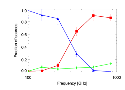
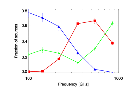
Fig. 15 shows the fraction of sources (like Fig. 8) by type (dusty, synchrotron, and now intermediate) as a function of frequency computed for sources above 80 % completeness. The fraction is at most 13 %, and is on average around 7 %. The intermediate source population thus has no impact on our number counts by type.

We conclude that a genuine population of intermediate sources exist (i.e. having both a thermal dust emission component and a synchrotron component) but its contribution in number is less than typically 10 % (Fig. 15). Notice that a free-free emission can also play a role in the spectrum flattening around 100 GHz (Peel et al., 2011).

We notice, however, that this intermediate populations lies at the faint end of the flux distribution (i.e. they usually are among the faintest sources of our sample). To investigate further if the presence of intermediate sources is linked to the level of photometric noise, we performed the classification on our whole sample, thus including sources at fluxes below the 80 % completeness limit. The results, shown in Fig. 16, indicates that the higher the photometric noise the more sources are classified as intermediate.

When using the total sample (i.e. with sources fainter that the 80 % completeness cut), the fraction of intermediate sources increases, but those sources are always at the faint end of the flux distribution: the effect of the photometric noise is thus mainly responsible for the uncertain classification. This emphasises that we should use highly-complete samples for such statistical analysis, in order not to be biased towards mis-classification.

Figure 16: Like Fig. 15, the fraction of source type (dusty, red squares; synchrotron, blue triangles; green diamonds, intermediate) as a function of frequency. The difference is that we have now included the whole catalogue, i.e. including sources affected by more photometric noise below the 80 % completeness limit cut. The effect of increasing noise is to induce more sources to be classified as intermediate.

Appendix B Some peculiarities; individual sources or groups of sources

While the SEDs of some particular sources have been published in the Planck early papers Planck Collaboration XIV (2011); Planck Collaboration XV (2011); Planck Collaboration XVI (2011), we review here some specific sources detected at low or high frequency, but with unexpected classifications.

B.1 Low-frequency dusty galaxies

There are seven low-frequency sources (three detected at 100 GHz and four at 143 GHz) that are classified as dusty galaxies. This kind of classification is not necessarily expected, unless we detect local galaxies showing both radio and infrared components. For this reason we check them individually.

1) PLCKERC100 G062.69$-$14.07: There is no radio identification in NVSS & GB6 or in NED, and no detection at LFI frequencies. This source is likely correctly classified as a dusty galaxy.

2) PLCKERC100 G140.41$-$17.39: This source is found with NED to be NGC 891. There is no LFI detection, but detections in NVSS/GB6. We might be seeing two spectral components (dusty and synchrotron) of this nearby galaxy.

3) PLCKERC100 G141.42+40.57: This is NGC3034 (M82). As above we are sensitive to both components of this nearby and well-studied galaxy.

4) PLCKERC143 G001.33$-$20.49: No LFI detection nor radio identification. This source is correctly classified as a dusty galaxy.

5) PLCKERC143 G148.59+28.70: This source is likely a blazar with an almost flat spetrcum at high frequencies and detections in NVSS and GB6. This source is likely incorrectly classified as dusty, because of the small jump in flux at 545 GHz.

6) PLCKERC143 G236.47$-$14.38: No LFI detection nor radio identification. This source is correctly classified as a dusty galaxy.

7) PLCKERC143 G349.61$-$52.57: No LFI detection. At 0.2 to 20 GHz it is identified as a flat-spectrum source but its high-frequency spectrum shows a clear dusty behaviour. This source is correctly classified as a dusty galaxy, although a clear radio component is detected.

B.2 High frequency synchrotron galaxies

There are four sources classified at synchrotron sources at 857 GHz. We also check them individually.

1) PLCKERC857 G206.80+35.82: This is a confirmed blazar detected with WMAP . This source is correctly classified as synchrotron-dominated.

2) PLCKERC857 G237.75$-$48.48: This is a confirmed blazar detected with WMAP and ATCA. This source is correctly classified as synchrotron-dominated.

3) PLCKERC857 G250.08$-$31.09: This is a confirmed blazar detected with WMAP and ATCA. This source is correctly classified as synchrotron-dominated.

4) PLCKERC857 G148.24+52.44: This is NGC 3408, quite faint for Planck at high frequencies (812 mJy at 857 GHz and not detected at 545 GHz). This source, although in our sample defined in Sect. 2.3, was not used in the number counts because of the low completeness level at this flux density.

B.3 Bump at 4 Jy at 545 GHz in the medium zone

As discussed in Sect. 4 and shown in Fig. 17, there is an excess of 545 GHz sources in the medium zone at 4 Jy, which is also seen at 857 GHz at 10 Jy and at 353 GHz at 1 Jy. This bump is created at 545 by 18 sources (between 3 and 5 Jy). Among the sources, we find NGC 3147, NGC 4449, NGC 4217, NGC 3992, NGC 4088, NGC 4096, NGC 4051, NGC 3631, NGC 3938, IC 0750, NGC 4244, NGC 3726, NGC 4214, NGC 7582 and NGC 7552. At 857 GHz, we find 20 sources between 7.6 and 12 Jy, with many in common with the list above. These sources are not physically associated and are spread over a large surface of the sky, although the majority lie around (150 deg., 60 deg.) in Galactic coordinates.

Figure 17: Planck differential number counts (total, dusty and synchrotron) at 6 frequencies between 100 and 857 GHz, normalized to the Euclidean, for each zone (filled circles): deep (red), medium (green) and shallow (blue). Diamonds are from Planck HFI Planck Collaboration XIII (2011), triangles from Herschel SPIRE (Oliver et al., 2010; Clements et al., 2010) and BLAST Bethermin et al. (2010b). The bump at 4 Jy at 545 GHz (and at 10 Jy at 857 GHz) in the medium zone is discussed in Sect. B.3.

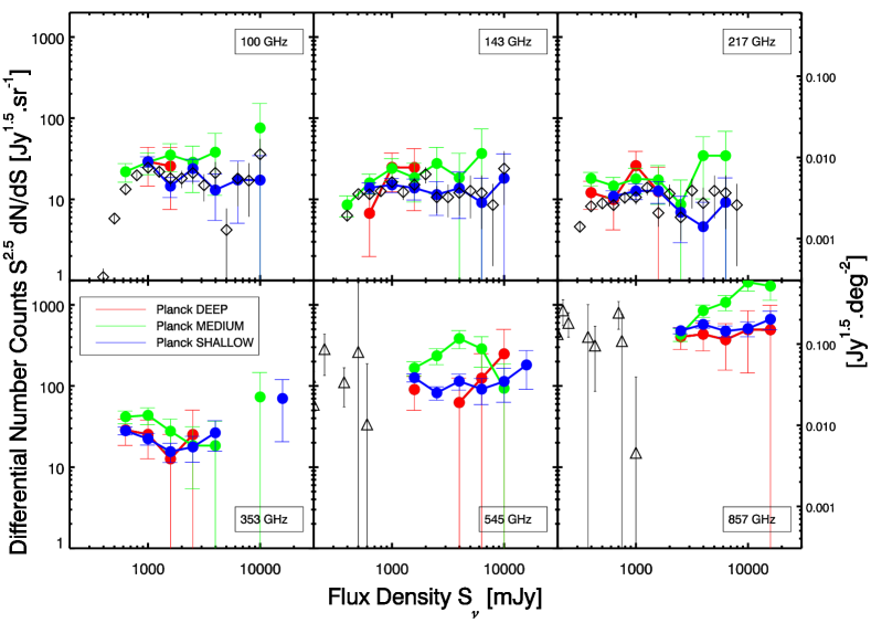
Appendix C Number counts by zone

Fig. 17 shows the number counts for each of the three zones: deep, medium, and shallow. This illustrates the sample variance, as mentioned in Appendix B.3.

Since, with the exception of one zone at 545 GHz, there is little difference between the counts in different zones, this figure also demonstrates that the weight given to each zone in calculating the total number counts has little influence on the result.