An Adaptive Online Ad Auction Scoring Algorithm for Revenue Maximization

Keywords: ad auction, sponsored search, adaptive algorithms, search engines, revenue maximization

1 Introduction

Sponsored search becomes an easy platform to match potential consumers’ intent with merchants’ advertising. Advertisers express their willingness to pay for each keyword in terms of bids to the search engine. When a user’s query matches the keyword, the search engine evaluates the bids and allocates slots to the advertisers that are displayed along side the unpaid algorithmic search results. The advertiser only pays the search engine when its ad is clicked by the user and the price-per-click is determined by the bids of other competing advertisers.

It seems natural to assume that the number of clicks an ad will get when displayed depends on some ad-specific factors. For example, when a potential buyer searches the key word “tennis racquet", an ad with “The Lowest Prices Guaranteed!" seems to be more intriguing and more likely to result in a click than an ad with “Save on Tennis Racquets". Besides, an online tennis store that has built a high reputation among the internet shoppers is more likely to attract more clicks than an online tennis store that keeps leaving customers negative experiences. There are many other measures of “ad quality" search engines may also consider in deciding which ads to display and at which positions.

These measures are incorporated into an “ad quality" scoring system that is widely used by the major search engines. For example, Google ranks ads by bid times the corresponding ad-quality score. When the ad-quality score of each advertiser is interpreted as the expected number of clicks the corresponding ad can generate once it is displayed, then the ads are ranked in the order of their expected revenue. This interpretation of the ad-quality score conveys a message to the advertisers: the search engine wants the higher ranked slots, those more likely to receives clicks, to go to the ads expected to generate higher revenues for it. It is not strange that all search engines’ goal in selling the ad slots is revenue maximization, but how do they achieve the goal through the ad-quality scoring remains a secrete to the advertisers. A simple example can show that, though intuitively appealing, ranking ordered by bid times expected click-through rate might not be the optimal ranking to generate maximum revenue for the search engine. Then two problems become interesting: What is a good scoring strategy for the search engine to maximize its revenue? Does the interpretation of the ad-quality score truly represents what the ad-quality score does in the process of revenue maximization?

In this paper, we study the scoring strategy of the search engine for the purpose of revenue maximization. Section 2 gives the preliminaries needed for our analysis. After specifying the ad auction model rules, notations and the related literature, we show some ad scoring examples that motivated this work. In Section 3, we focus on the complete information setting, where advertisers’ values are known. Our analysis shows that when there are more advertisers than slots, there is a scoring strategy that induces a Nash equilibrium formed by the set of truthful bids. Under such an equilibrium, the search engine takes all the social surplus and the socially optimal ranking of the advertisers is the optimal ranking for maximizing the search engine’s revenue. Furthermore, we show that under such a truthful bidding Nash equilibrium, when the click-through rate for an advertiser at a certain slot takes a product form of an ad-specific factor and a position-specific factor, there exists a $0\left(N^{2}\right)$ time algorithm to find the socially optimal ranking of the advertisers which also maximize the search engine’s revenue.

In Section 4, we move to the incomplete information case where advertisers’ values are not known by the search engine. Based on some rational advertisers behavior arguments, we propose an adaptive online algorithm that dynamically scores ads to reveal advertisers’ values and to manipulate their rankings to maximize the search engine’s total revenue. In Section 5, we test the algorithm under the 8-slot sponsored ads setting used by Google, Microsoft (Bing.com) and Yahoo! and simulation results show that the performance of the algorithm agrees very well with our theoretical analysis. We conclude the paper in Section 6.

2 Preliminaries

2.1 Auction rules

We focus on a single keyword slot auction, where there are $N$ advertisers competing for $S$ slots. Without loss of generality, we assume $S\geq N$, since redundant slots can remain blank. Let $i=1,...,N$ index advertisers and $j=1,...,S$ index slots. Let $v_{i},b_{i}$ be the value, bid of advertiser $i$ for a particular keyword and $p_{i,j}$ be the price per click advertiser $i$ pays at slot $j$. Let $e_{i}\,>0$ be the ad-quality score the search engine assigns to advertiser $i$ to represent a measure of the predicted click-through rate advertiser $i$ will generate and $x_{i,j}$ be the actual click-through rate advertiser $i$ receives at slot $j$ per hour.

We follow the rules of the auction described in [1] by Varian that are used by the major search engines.

(1) Each advertiser $i$ chooses a bid $b_{i}$.

(2) The advertisers are ordered by bid times predicted click-through rate $b_{i}\times e_{i}$.

(3) The price that advertiser $i$ pays for a click is the minimum necessary to retain its position.

(4) If there are fewer bidders than slots, the last bidder pays a reserve price $p_{r}$.

2.2 Previous literature

When $e_{i}\equiv 1$ for all the advertisers, the above described auction becomes the Generalized Second Price Auction (GSP) first developed and adopted by Google in 2002, where advertisers are ranked by their bids and the advertiser assigned slot $j$ pays the price per click equal to the bid of the advertiser assigned slot $j+1$. Early studies on some basic properties of GSP are independently reported by Edelman et al. [2] and Varian [3].

In their analysis, the ad auction problem is modeled as a game where each advertiser is a player who uses bidding as strategy to maximize its surplus, i.e., the value of the clicks it receives minus the price it pays the search engine for those clicks. The game becomes of special interest when in equilibrium, each advertiser prefer its current slot to other slots and has no incentive to change how it is bidding. Here is the formal definition.

Definition 1. Given the advertisers’ value $\left(v_{1},...,v_{N}\right)$, a Nash equilibrium is the set of bids so that given these bids, no advertiser has an incentive to change its bid. Specifically, a Nash Equilibrium (NE) satisfies, for any advertiser $i$,

$$\left(v_{i}-p_{i,j}\right)x_{i,j}\geq\left(v_{i}-p_{i,j^{\prime}}\right)x_{i,j^{\prime}}\text{ \ \ for all slots }j^{\prime}\neq j.$$

Varian in [3] studies the bidding behavior under the GSP auction and shows every advertiser has a range for the bid to place to maintain its current position. He derives many meaningful results when the advertisers’ bidding profile and the corresponding pay per click prices reach a subset of Nash Equilibrium, namely the symmetric Nash equilibrium (SNE). Based on the lower and upper bounds of the SNE bids, Varian derives the lower and upper bounds of the total revenue a search engine can obtain [3] and further estimates advertisers’ surpluses based on the prices per click they pay [1].

Lahaie [4] gives a good study on the two auctions, one with all $e_{i}$ being equal and the other with $e_{i}$ representing the expected click-through rate and names them “rank by bid" and “rank by revenue" respectively. Both complete and incomplete settings are considered and estimation of the search engine’s revenue is given. However, there is no analysis of revenue-maximizing scoring strategy for the searching engine.

The most relevant work to ours can be found in Liu and Chen [Liu06] where the “ad-quality" score is referred to as the “weighting factor". They study in the incomplete information setting both the “efficient" weighting factor that maximize the total social surplus and the “optimal" weighting factor that maximize the search engine’s revenue. However, they only focus on the ad auction model with one slot and the quality type for the advertisers is binary (high or low), while we study multiple advertisers and slots and obtain the corresponding results through equilibrium analysis in the complete information setting.

2.3 Motivating Examples

In [3] Varian gives the lower and upper bounds of the total revenue a search engine can obtain by selling the ad positions but does not discuss whether this revenue under the symmetric Nash equilibrium is optimal. Here, a simple example shows that when the ad-quality score $e_{i}$ accurately predicts the click-through rate for each advertiser $i$, the resulting ranking based on $b_{i}\times e_{i}$ might not generate the maximum revenue for the search engine.

Table 1 gives the different click-through rates three advertisers Coke, Pepsi and Dr. Pepper will get under different rankings for the key word “soda drink" in a 3-slot ad auction. Let us assume that Coke and Pepsi are the only two advertisers that sell cola and potential buyers looking for cola will either click on Coke or Pepsi. Further assume Coke has a bigger brand name and whenever placed at the same position will always receive a higher click-through rate than Pepsi ($x_{Coke,j}>x_{Pepsi,j}$).

Table 1: Click-through rates under different rankings for Coke, Pepsi and Dr. Pepper.

Advertiser Rank $$x_{i,j}$$ Rank Rank Rank Rank Rank

Coke 1 70 1 80 2 50 2 70 3 40 3 50

Pepsi 2 30 3 20 1 50 3 30 1 60 2 50

Dr. Pepper 3 20 2 30 3 20 1 35 2 30 1 35

Tables 2-4 give the advertisers’ bids, surpluses and the search engine’s revenue generated under 3 different scoring and ranking scenarios. Drink X is always the one that does not get a slot.

Table 2: Bids and quality scores for the key word “soda drink", senario 1.

Advertiser $$e_{i}$$ Rank

Coke 70 $0.05 3.5 1 $0.03 $0.10 70 $4.9 $2.1

Pepsi 30 $0.07 2.1 2 $0.067 $0.10 30 $1.0 $2.0

Dr. Pepper 20 $0.10 2.0 3 $0.07 $0.10 20 $0.60 $1.4

Drink X 20 $0.07 1.4 4 $0 $0.07 0 $0 $0

Table 3: Bids and quality scores for the key word “soda drink", senario 2.

Advertiser $$e_{i}$$ Rank

Pepsi 50 $0.07 3.5 1 $0.05 $0.10 50 $2.5 $2.5

Coke 50 $0.05 2.5 2 $0.04 $0.10 50 $3.0 $2.0

Dr. Pepper 20 $0.10 2.0 3 $0.07 $0.10 20 $0.6 $1.4

Drink X 20 $0.07 1.4 4 $0 $0.07 0 $0 $0

Table 4: Bids and quality scores for the key word “soda drink", senario 3.

Advertiser $$e_{i}$$ Rank

Pepsi 40 $0.08 3.2 1 $0.06125 $0.10 50 $1.875 $3.125

Coke 50 $0.05 2.5 2 $0.04 $0.10 50 $3.0 $2.0

Dr. Pepper 20 $0.10 2.0 3 $0.07 $0.10 20 $0.6 $1.4

Drink X 20 $0.07 1.4 4 $0 $0.07 0 $0 $0

In scenario 1, Coke, Pepsi and Dr. Pepper are enjoying surpluses of $4.9, $1.0 and $0.60 per hour respectively and generating $2.1, $2.0 and $1.4 per hour for the search engine. In such a setting, Dr. Pepper does not have an incentive to move up in the ranking or otherwise it needs to pay at least $0.105 per click which is greater than its value of $0.10 per click. Dr. Pepper does not have an incentive to move down either since that will make its surplus 0. Coke and Pepsi would also prefer their current positions. To see this, if Coke moves down one slot, it needs to pay at least $0.0286 and receives 50 clicks per hour. This ends up with a surplus of $3.5714, which is less than the $4.9 surplus it is making now. Similarly, if Pepsi moves down one slot, its surplus becomes $0.8 and if Pepsi moves up on slot, its surplus is -$0.8333, both are less than its current surplus $1.0. Finally, Drink X does not want to move up one slot because it has to pay $0.10 which will make its current 0 surplus being negative. Therefore, scenario 1 is an NE. Further more, the quality scores for Coke, Pepsi  and Dr. Pepper perfectly predict the actual click-through rates after the ranking and reflect the fact that Coke has a relatively higher “ad quality" than Pepsi. However, this “full mark" scoring generates the lowest revenue among the 3 scenarios.

In scenario 2, quality scores for Coke and Pepsi are changed to be the same of 50 with the remaining advertisers’ scores unchanged. This change results in the swap of ranking for Coke and Pepsi compared with scenario 1. It is easy to check scenario 2 also represents an NE in advertisers bidding and that bidding profile is exactly the same as in scenario 1, but with $0.4 more revenue generated for the search engine. Here, quality scores also perfectly predict the actual click-through rates but do not show the fact that Coke has a better “ad quality" than Pepsi.

Tables 2-3 together show that if the purpose of scoring is to accurately predict the click-through rates and thus the expected revenue from each advertiser, scores do not necessarily need to reflect the true relative “ad qualities".

Scenario 3 generates the highest revenue for the search engine among the 3 scoring profiles and forms another NE with an increased bid of Pepsi from $0.07 to $0.08. This increase in bid is a result of the decreased ad-quality score for Pepsi compared with scenario 2. It is interesting to note that increasing the bid from $0.07 to $0.08 does not increase Pepsi’s pay per click rate but eliminates Coke’s incentive of moving up one slot. In this scenario, the scores reflect the relative “ad qualities" for Coke and Pepsi but do not agree with the actual click-through rates.

The above described simple example shows many interesting observations about ad-quality scoring and ranking.

1. Rankings can be changed by manipulating the ad-quality scores $e_{i}$ for corresponding advertisers to serve the purpose of increasing the search engine’s revenue. This can be done with (i.e., scenario 3) or without (i.e., scenario 2) changing the bidding profile of the advertisers.

2. The scoring profile that gives the search engine more revenue does not necessarily need to reflect better the relative “ad-qualities" of advertisers or the actual click-through rate after the ranking.

3. Changes in the ad-quality scores can result in the advertisers’ bids moving from one NE to another. Any increase in the search engine’s revenue comes from the decrease in the advertisers’ total surpluses.

3 Scoring Strategy in Complete Information Setting

The nature of the ad-quality score and the dynamic interactions between the search engine’s scoring and the advertisers bidding make search engine revenue maximization far from a straightforward business. Under the same scoring profile, there might be multiple NE bidding sets and multiple resulting rankings. The existence of multiple equilibria also adds to the difficulty in reasoning about the search engine revenue generated by the ad auction, since it depends on which equilibrium (potentially from among many) is selected by the advertisers. In light of this, we choose to start our analysis with the socially optimal ranking, which is independent with the search engine and advertisers’ behavior. Besides, the maximum social surplus obtained under the socially optimal ranking serves naturally as an upper bound for the search engine’s maximum achievable revenue.

Let us add fake slots with click-through rates $x_{\cdot,j}=0$ for $j=S+1,...,N$ to make the total number of slots match the total number of advertisers. Let $\sigma$ be a one-to-one permutation function from the advertisers’ index set $\left\{1,...,N\right\}$ to the slots index set $\left\{1,...,N\right\}$, so that for advertiser $i$, $\sigma\left(i\right)$ gives its rank. Let $\Pi_{i}\left(\sigma\right)$ be the surplus for advertiser $i$ with respect to ranking $\sigma$ and $\Pi_{ad}\left(\sigma\right)=\sum_{i=1}^{N}\Pi_{i}\left(\sigma\right)$ be the corresponding total surpluses for all advertisers. For any permutation $\sigma$, the social surplus $\Pi_{social}\left(\sigma\right)$ is the sum of total advertisers’ surpluses $\Pi_{ad}\left(\sigma\right)$ and the search engine’s surplus $\Pi_{se}\left(\sigma\right)$, where

$$\Pi_{social}\left(\sigma\right) = \Pi_{ad}\left(\sigma\right)+\Pi_{se}\left(\sigma\right)$$

$$= \sum_{i=1}^{N}\left(v_{i}-p_{i,\sigma\left(i\right)}\right)x_{i,\sigma\left(i\right)}+\sum_{i=1}^{N}p_{i,\sigma\left(i\right)}x_{i,\sigma\left(i\right)}$$

$$= \sum_{i=1}^{N}v_{i}x_{i,\sigma\left(i\right)}$$

Definition 2. A socially optimal ranking $\sigma^{\ast}$ is the permutation that maximize the social surplus, where

$$\sigma^{\ast}=\arg\max_{\sigma}\Pi_{social}\left(\sigma\right)=\arg\max_{\sigma}\sum_{i=1}^{N}v_{i}x_{i,\sigma\left(i\right)}$$

Before we move on to analyze the scoring strategy for the search engine, we assume the goal for any advertiser is surplus maximization.

Definition 3. Given the values of the advertisers $\left(v_{1},...,v_{N}\right)$, an equalizing scoring profile for the search engine is defined as a scoring profile $e^{\ast}=\left(e_{1}^{\ast},...,e_{N}^{\ast}\right)$ such that $e_{i}^{\ast}v_{i}=e_{i^{\prime}}^{\ast}v_{i^{\prime}}$ for all $i\neq i^{\prime}$.

By definition, an equalizing scoring profile always exists, i.e., $e_{i}^{\ast}=1/v_{i}$ for all $i$. If $e^{\ast}$ is an equalizing scoring profile, for any $k>0$, $ke^{\ast}$ is also an equalizing scoring profile. The following Theorem 1 shows that where there are more advertisers than slots with $N>S$, under an equalizing scoring profile, the set of truthful bids forms a Nash equilibrium. Furthermore, in such an NE, the search engine extracts all the surpluses from the bidders making the search engine’s surplus equal the total social surplus.

Theorem 1. When there are more advertisers than slots, $N>S$, under any equalizing scoring profile $e^{\ast}$, the set of truthful bids $b^{\ast}=\left(v_{1},...,v_{N}\right)$ is an NE. The surplus for each advertiser $\Pi_{i}=0$ and the search engine’s surplus $\Pi_{se}=\Pi_{social}$. The resulting ranking can be any permutation $\sigma$ of the advertisers.

Proof. Given the set of truthful bids $b^{\ast}=\left(v_{1},...,v_{N}\right)$, we have $\ b_{i}=v_{i}$ and thus the price advertiser $i$ paying is $p_{i}=v_{1}e_{1}/e_{i}=v_{i}$, for all $i=1,...,N$. Without loss of generality, suppose advertiser $1$ bids above its value $v_{1}$. In this case, it is assigned the top slot and the price for the top slot changes to $p_{1,1}=e_{i}v_{i}/e_{1}=v_{1}$ which leads to no positive surplus. Hence, this deviation is not strictly profitable. If an advertiser bids below its value then it loses a slot if it had been allocated one since $N>S$, or otherwise, it continues to have no slot allocated. Again, no positive surplus. This shows the set of bids $b^{\ast}=\left(v_{1},...,v_{N}\right)$ is an NE.

Each advertiser’s surplus $\Pi_{i}\left(\sigma\right)=\left(v_{i}-p_{i,\sigma\left(i\right)}\right)x_{i,\sigma\left(i\right)}=0$. Since this is true for any permutation $\sigma$, any permutation $\sigma$ can be the resulting ranking from the set of truthful bids $b^{\ast}=\left(v_{1},...,v_{N}\right)$.                                                                     $\blacksquare$

In the proof of Theorem 1, it shows that under an equalizing scoring profile $e^{\ast}$, the set of truthful bids forms an NE but does not indicate whether this NE is unique. It is easy to check that a set of bids where one advertiser bids above its value while all other advertisers bids their values also represents an NE and therefore, the truthful bidding set is not the unique NE that an equalizing scoring profile $e^{\ast}$ will induce.

In Theorem 2, we show that when $N>S$, under the equalizing scoring profile $e^{\ast}$ and the set of truthful bids $b^{\ast}$, among the $N!$ possible NE permutations, the one that maximize the search engine’s surplus is the socially optimal ranking $\sigma^{\ast}$.

Theorem 2. When $N>S$, under the equalizing scoring profile $e^{\ast}$, the set of truthful bids $b^{\ast}$ and the socially optimal ranking $\sigma^{\ast}=\arg\max_{\sigma}\sum_{i=1}^{N}$ $v_{i}x_{i,\sigma\left(i\right)}$ together form an NE where each advertiser has $0$ surplus and the search engine has its maximum revenue equal to the maximum social surplus $\Pi_{se}^{\ast}=\sum_{i=1}^{N}$ $v_{i}x_{i,\sigma^{\ast}\left(i\right)}$.

Proof. The results follow directly from Theorem 1.          $\blacksquare$

It is commonly assumed that the expected click-through rate of advertiser $i$ in slot $j$ can be written as the product of an ad-specific factor $q_{i}$ and a position-specific factor $s_{j}$, specifically $x_{ij}=q_{i}s_{j}$. While this product form is not generally true in practice, it makes the ad-specific factor and the position specific factor separable and usually leads to particularly simple analytical results.

Assumption 1. The expected click-through rate advertiser $i$ gets in slot $j$ can be expressed in a product form $x_{ij}=q_{i}s_{j}$, where $q_{i}\geq 0$ is an ad-specific factor and $s_{j}\geq 0$ is a position-specific factor. Furthermore, we assume the position-specific factors are in a descending order with respect to the ranking of the slots, that is $s_{j}>s_{j^{\prime}}$, for all $j<j^{\prime}$.

Theorem 3. Under Assumption 2, a permutation $\sigma$ is the socially optimal ranking iff for any adjacently ranked advertisers $\left(i,i^{\prime}\right)$, where $\sigma\left(i\right)=\sigma\left(i^{\prime}\right)-1$, $v_{i}x_{i,\sigma\left(i\right)}+v_{i^{\prime}}x_{i^{\prime},\sigma\left(i^{\prime}\right)}\geq v_{i}x_{i,\sigma\left(i^{\prime}\right)}+v_{i^{\prime}}x_{{}_{i,}\sigma\left(i\right)}.$

Proof. $``\Rightarrow"$. Obvious by the definition of social optimality.

$``\Leftarrow"$. Substituting $\sigma\left(i^{\prime}\right)=\sigma\left(i\right)+1$, $x_{i},_{\sigma\left(i\right)}=q_{i}s_{\sigma\left(i\right)}$ and $x_{i^{\prime}},_{\sigma\left(i^{\prime}\right)}=q_{i^{\prime}}s_{\sigma\left(i^{\prime}\right)}$ into $v_{i}x_{i,\sigma\left(i\right)}+v_{i^{\prime}}x_{i^{\prime},\sigma\left(i^{\prime}\right)}\geq v_{i}x_{i,\sigma\left(i^{\prime}\right)}+v_{i^{\prime}}x_{{}_{i,}\sigma\left(i\right)}$, we have

$$v_{i}q_{i}s_{\sigma\left(i\right)}+v_{i^{\prime}}q_{i}s_{\sigma\left(i\right)+1} \geq v_{i}q_{i}s_{\sigma\left(i\right)+1}+v_{i^{{}^{\prime}}}q_{i^{\prime}}s_{\sigma\left(i\right)}$$

$$v_{i}q_{i}\left(s_{\sigma\left(i\right)}-s_{\sigma\left(i\right)+1}\right) \geq v_{i^{\prime}}q_{i^{\prime}}\left(s_{\sigma\left(i\right)}-s_{\sigma\left(i\right)+1}\right)$$

By the descending property of the position-specific factors, we have $s_{\sigma\left(i\right)}-s_{\sigma\left(i\right)+1}>0$, which gives $v_{i}q_{i}\geq v_{i^{\prime}}q_{i^{\prime}}$. Since this is true for all adjacently ranked advertisers $\left(i,i^{\prime}\right)$, it means the permutation $\sigma$ is a ranking based on the descending order of $v_{i}q_{i}$. Without loss of generality, we re-index the advertisers such that for all $i<i^{\prime}$, $v_{i}q_{i}\geq v_{i^{\prime}}q_{i^{\prime}}$. Then $\sigma\left(i\right)=i$, meaning advertiser $i$ is assigned to slot $i$ for all $i=1,...,N$.

Now let us assume the socially optimal ranking is $\sigma^{\ast}\neq\sigma$. Then there is at lease one $i$, such that $\sigma^{\ast}(i)\neq i$. Let $k=\min\left\{i|\sigma^{\ast}(i)\neq i\right\}$ and $k^{\prime}$ be the index of the advertiser such that $\sigma^{\ast}\left(k^{\prime}\right)=k$. Define another permutation $\sigma^{\prime}$ that only differs with $\sigma^{\ast}$ by swapping the ranks of advertisers $k$ and $k^{\prime}$. Specifically, $\sigma^{\prime}\left(k\right)=\sigma^{\ast}\left(k^{\prime}\right)$, $\sigma^{\prime}\left(k^{\prime}\right)=\sigma^{\ast}\left(k\right)$ and $\sigma^{\prime}\left(i\right)=\sigma^{\ast}\left(i\right)$, for all $i\neq k,k^{\prime}$. The social surplus under the new permutation $\sigma^{\prime}$ is

$$\Pi_{social}\left(\sigma^{\prime}\right)$$

$$= \Pi_{social}\left(\sigma^{\ast}\right)-v_{k}x_{k,\sigma^{\ast}\left(k\right)}-v_{k^{\prime}}x_{k^{\prime},\sigma^{\ast}\left(k^{\prime}\right)}$$

$$+v_{k}x_{k,\sigma^{\prime}\left(k\right)}+v_{k^{\prime}}x_{k^{\prime},\sigma^{\prime}\left(k^{\prime}\right)}$$

$$= \Pi_{social}\left(\sigma^{\ast}\right)+v_{k}q_{k}\left(s_{\sigma^{\prime}\left(k\right)}-s_{\sigma^{\ast}\left(k\right)}\right)$$

$$-v_{k^{\prime}}q_{k^{\prime}}\left(s_{\sigma^{\ast}\left(k^{\prime}\right)}-s_{\sigma^{\prime}\left(k^{\prime}\right)}\right)$$

$$= \Pi_{social}\left(\sigma^{\ast}\right)+\left(v_{k}q_{k}-v_{k^{\prime}}q_{k^{\prime}}\right)\left(s_{\sigma^{\ast}\left(k^{\prime}\right)}-s_{\sigma^{\ast}\left(k\right)}\right)$$

$$\geq \Pi_{social}\left(\sigma^{\ast}\right)$$

The last inequality follows the fact that $k$ is the first advertiser that does not satisfy $\sigma^{\ast}(i)=i$ and therefore $v_{k}q_{k}-v_{k^{\prime}}q_{k^{\prime}}\geq 0$ and $s_{\sigma^{\ast}\left(k^{\prime}\right)}-s_{\sigma^{\ast}\left(k\right)}>0$. Since $\sigma^{\ast}$ is a socially optimal ranking, $\sigma^{\prime}$ is also a socially optimal ranking. By sequentially swapping all the out-of-place $i$s, we will finally obtain the permutation $\sigma\left(i\right)=i$ and $\Pi_{social}\left(\sigma\right)\geq\Pi_{social}\left(\sigma^{\ast}\right)$. Therefore, $\sigma\left(i\right)=i$ is the socially optimal permutation.                                                                        $\blacksquare$

The proof of Theorem 3 shows a constructive way of finding the socially optimal ranking under the equalizing scoring profile by sequentially swapping neighboring ads seeking improvement of the total revenue until no improvement can be made. The is an example where local search leads to global optimum and the search algorithm costs no more than a bubble sort!

Theorems 1-3 all together serve as the theoretical foundation for constructing the adaptive online ad-auction scoring algorithm shown in the next section.

4 An adaptive online ad-auction scoring algorithm

In this section, we develop an adaptive online ad-auction scoring algorithm to maximize the search engine’s revenue in the incomplete information case where the values of the advertisers are not known to the search engine.

4.1 Arguments on Advertisers Behavior

Before we move on to the algorithm construction, we make two arguments of the advertiser behavior based on the surplus maximization assumption for each advertiser

Argument 1. An advertiser will not bid above its true value.

We have shown in the complete information setting, at least with the equalizing scoring profile, one advertiser bids above its value and other bids their values is an NE and therefore overbidding is not an infeasible strategy. However, in practice, the search engine does not provide an advertiser with its own or others “ad-quality" scores or others bids. While over time, an advertiser is likely to learn all the information to identify that itself is in an equilibrium, try bidding over its value always has a chance of being penalized with negative surplus.

Argument 2. If being left out without having a slot, an advertiser will bid its true value.

By surplus maximization, the goal for any advertiser joining the auction is to get a slot and maximize its surplus. Since the bid is an advertiser’s only strategy to get itself a slot, when keeps missing a slot, it will at least try to express its maximum willingness to pay to see whether that can get it a slot.

Though we are not proving the above two arguments, they are not unreasonable in practice, especially when the scoring mechanism is kept totally secret by the search engine. In what follows, we propose an adaptive online ad auction scoring algorithm for the search engine revenue maximization taking advantage of the above two arguments. Though the results we get may be too ideal in reality, it illustrates a possible approach to reveal advertisers’ values and shows insights into what will happen when the search engine have a way to accurately estimate advertisers’ values.

4.2 Algorithm Construction

Theorems 1-3 show that in complete information setting, how a search engine may maximize its revenue, 1) apply an equalizing scoring profile; 2) induce truthful bidding; 3) find the socially optimal ranking.

To apply the equalizing scoring strategy, the search engine must have a mechanism to find out first the values of the advertisers. Once the values are found, an optimization procedure is needed to search for the optimal ranking to maximize the revenue. Accordingly, we have in our scoring algorithm a “value revealing" module and an “optimal rank searching" module to implement these two functionalities simultaneously. The idea is based on the following.

1. We divide the set of advertisers into two sets, one set $U$ contains all the advertisers whose values are not known yet, the other set $V=\left\{1,...,N\right\}\backslash U$ contains those whose values are revealed already. By Argument 2, after the first NE is reached, $V\neq\phi$.

2. The value revealing module applies equalizing scoring strategy to all the advertisers in $V$ to make their $e_{i}\times v_{i}$ equal (and therefore everyone is forced to bid their true value) and then gradually increases $e_{i}s$ (while making sure all $e_{i}\times v_{i}$ increase the same amount) to push out surpluses from the advertisers in set $U$. Since the ad-quality scores for advertisers in $U$ are not increased, an advertiser in $U$ will ultimately be forced to lose its slot and reveal its value to the search engine. This is when the advertiser leaves the set $U$ and enters $V$.

3. Once a new advertiser $i$ enters $V$, the optimal rank searching module applies sequential swaps to the new member $i$ and its neighboring advertiser $j$ by making a small $\varepsilon>0$ difference between $e_{i}b_{i}$ and $e_{j}b_{j}$. The swap will keep going until no increase in the search engine’s revenue can be obtained. By Theorem 3, when advertisers enter the set $V$ gradually, the optimal rank searching module makes sure all the advertisers in the set $V$ are ordered in a way that is consistent with the social optimal ranking.

4. Any time an advertiser’s score is changed, the algorithm will let all the advertisers settle into a new NE. By the way how the value revealing module works, for any $i\in V$ and $j\in U$, we always have $e_{i}v_{i}<e_{j}v_{j}$, and the auction rules will make sure the permutation $\sigma$ resulted from NE has $\sigma\left(i\right)>\sigma\left(j\right)$.

5. The algorithm continues until the set $U$ is emptied. This is when all the advertisers’ values are revealed and resulting permutation $\bar{\sigma}$ is the socially optimal ranking $\sigma^{\ast}$.

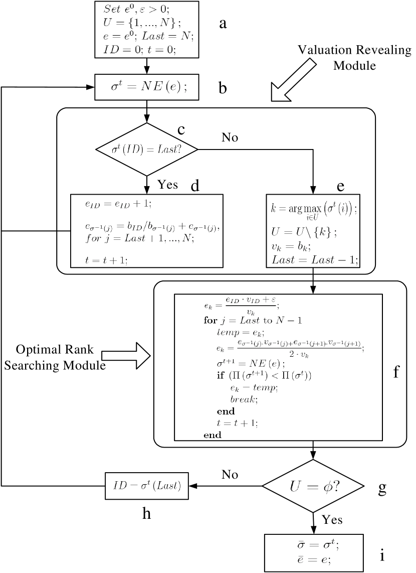
Figure 1: Flow chart for the adaptive scoring algorithm

Figure 1 illustrates the flow chart with pseudo code for the adaptive ad scoring algorithm. $\sigma^{-1}$ is the inverse function of $\sigma$ so that given a slot index $j\,$, $\sigma^{-1}\left(j\right)$ returns the index of the advertisers occupying slot $j$.

$ID$ is the index of the advertiser in the set $V$ that has the highest rank, where $ID=\arg\min_{i}\left\{\sigma\left(i\right)|i\in V\right\}$. $Last$ is the index of the slot that equals the total number of advertisers in set $U$ plus 1, where $Last=\left|U\right|+1$. $NE\left(\cdot\right)$ is a function that takes the input of a scoring profile $e=\left(e_{1},...,e_{N}\right)$, simulates the Nash equilibrium of advertisers’ bids and then returns a resulting permutation $\sigma$. $t$ keeps track of the total number of score adjustments needed for the algorithm.

Under Assumption 1 and by Theorems 1-3, the final ranking $\bar{\sigma}$ obtained by the proposed algorithm is the socially optimal ranking $\sigma^{\ast}$. The total search engine revenue $\Pi_{se}\rightarrow$ $\Pi_{social}\left(\sigma^{\ast}\right)$ as $\varepsilon\rightarrow 0$.

5 Empirical analysis: implementation and results

We test the proposed algorithm under the 8-slot sponsored ad setting used by Google, Microsoft (Bing.com) and Yahoo! with 9 advertisers. Given 8 slots, 9 advertisers, there will be $9!\approx 360,000$ click-through rate distribution vectors. We first show that our algorithm finds the social optimal ranking when the system parameters $v$, $q$ and $s$ take static values. We then show that in a dynamic environment, our algorithm is able to adapt to the changes of these parameters in a timely fashion.

Finally, we relax the assumption that the click-through rate takes a product form of a ad-specific factor and a position-specific factor and make the click-through rate also dependent on the relative positions among the advertisers. Under this new model for click-through rate, our algorithm can not claim optimality. However, we show by simulation that the maximum revenue for the search engine obtained by our algorithm is close to the optimal search engine revenue.

5.1 8-Slot Auction with Static System Parameters

We set the user value vector as $v=$(19, 8, 7, 6, 5, 4, 13, 12, 1), the position-specific factor vector as $s=$(65, 50, 40, 36, 30, 18, 12, 10, 0) and the ad-specific factor vector as $q=$(35, 45, 35, 20, 50, 20, 10, 70, 5). (we need these two vectors to generate the actual click through rates $x$ for different permutations). The socially optimal ranking for this scenario is $\sigma^{\ast}=$(2, 3, 5, 7, 4, 8, 6, 1, 9) and the optimal social surplus $\Pi_{social}(\sigma^{\ast})=123,180$.

We set the initial scores for all the advertisers to be $100$, i.e., $e^{0}=\left(100,...,100\right)$. The algorithm runs $338$ iterations (i.e., it adjusts the ad-quality scores 338 times) before it stops. We show in Table. 4 the output of the algorithm, where $\bar{b}_{i}$, $\bar{e}_{i}$, $\bar{p}_{i}$ denote the final bidding, ad-quality score and price for each advertiser $i$ respectively.

Table 4: Output of the algorithm for static case.
Advertiser $i$	rank $\bar{\sigma}(i)$	$\bar{b}_{i}\times\bar{e}_{i}$	$\bar{b}_{i}$	$\bar{p}_{i}$
1	2	1909	19	18.94
2	3	1903	8	7.97
3	5	1893.7247	7	6.997
4	7	1892.5	6	5.992
5	4	1895	5	4.997
6	8	1890	4	3.987
7	6	1893.125	13	12.995
8	1	1915	12	11.962
9	9	1886	1	0

We also obtain the final revenue for the search engine to be $\Pi_{se}(\bar{\sigma})=122,032.85$, which is $99.07\%$ of the social optimal revenue $\Pi_{social}({\sigma}^{\ast})=123,180$.

Our first observation is that the output ranking $\bar{\sigma}$ equals the social optimal ranking $\sigma^{\ast}$. The second observation is that the price $\bar{p}_{i}$ each advertiser $i$ pays almost equal to its individual value $v_{i}$, which means each advertiser has almost no surplus left. Combining the previous two observations, we conclude that the search engine gets almost all the surplus. We see that this is indeed the case when we compare $\Pi_{social}(\sigma^{\ast})$ and $\Pi_{se}(\bar{\sigma})$. The third observation is that $e_{i}\times b_{i}$ is ranked the same as the advertiser ranking, with the advertiser who ranks higher gets larger $e_{i}\times b_{i}$. This property ensures that the rule of the ranking is observed, i.e., the search engines should order the advertisers by $b_{i}\times e_{i}$.

Fig.2 shows the evolution of the values $e_{i}^{t}\times b_{i}^{t}$ for all advertisers and illustrates how our algorithm works. In this example, advertiser 9 has both the lowest value and ad-specific factor, therefore remains ranked last throughout the process. Advertiser $6$ has the next lowest value and is forced by the value revealing module to bid its value at approximately $t=150$. This is when the two trajectories $e_{6}^{t}\times b_{6}^{t}$ and $e_{9}^{t}\times b_{9}^{t}$ meet and advertiser 6 enters the set $V$ from then on. Then advertiser $5$, who has the third lowest value, is forced to bid its value at approximately $t=175$. This process goes on until at time $t=334$, when advertiser $1$, who has the highest value, is forced to bid its value. At this point, the $b_{i}^{t}\times e_{i}^{t}$ becomes almost equal for everyone.

We notice that advertisers join the set $V$ in the order of their values. However, the final rank $\bar{\sigma}$ is in the order of $q_{i}\times v_{i}$ by the work of the optimal rank searching module. The small $\varepsilon$ difference in $e_{i}\times b_{i}$ plays the role of maintaining the relative positions of the advertisers in $V$ according to the social optimal ranking. Because of this $\varepsilon$ difference in $e_{i}\times b_{i}$, the price each advertiser pays is slightly lower than its true value and therefore making the search engine’s revenue a little less than the total social surplus. This little gap can be view as a cost to the search engine in order to keep the advertisers ranked in the way it wants.

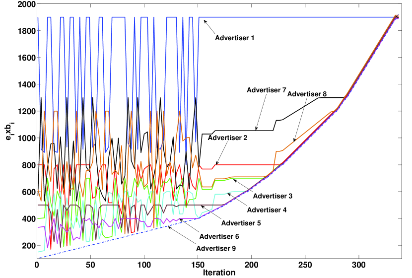
Figure 2: Evolution of $e_{i}\times b_{i}$ produced by the algorithm for all advertisers.

5.2 8-Slot Auction with Dynamic System Parameters

In this subsection, we show that once our algorithm has found a socially optimum ranking, it is able to track small changes in the individual value, the position-specific factor, or the ad-specific factor in a timely fashion.

In order to do so, we assume that these parameters are time varying, and we use $v^{u}$, $q^{u}$ and $s^{u}$ to denote the value of these parameters at time instance $u$, respectively. We are interested in the number of adjustments of the ad-quality scores the search engine needs to perform before the old optimum profile (optimal ranking and optimal scores) can adapt to the new system parameters and arrives at a new optimum profile.

Now, we generate the parameters at time $u$ by $v^{u}=\hat{v}+\epsilon_{v}^{u}$, $q^{u}=\hat{q}+\epsilon_{q}^{u}$, $s^{u}=\hat{s}+\epsilon_{s}^{u}$, where $\hat{v}$, $\hat{q}$ and $\hat{s}$ are the mean values of the parameters; $\epsilon_{v}^{u}$, $\epsilon_{q}^{u}$ and $\epsilon_{s}^{u}$ are the noisy realization to these parameters at time $u$; and $v^{u}$, $q^{u}$ and $s^{u}$ are the actual values these parameters take at time $u$.

The simulation setting is as follows. In order to compare the results obtained in the previous subsection, we choose $\hat{v}=$(19, 8, 7, 6, 5, 4, 13, 12, 1), $\hat{q}=$(65, 50, 40, 36, 30, 18, 12, 10, 5), $\hat{s}=$(35, 45, 35, 20, 50, 20, 10, 70, 0), which are the same as the corresponding static parameters in the previous subsection. We set $\epsilon_{q}\sim\mathcal{N}(0,36)$, $\epsilon_{s}\sim\mathcal{N}(0,25)$ and $\epsilon_{v}\sim\mathcal{N}(0,0.1)$. This setting implies position-specific factors are more volatile than the ad-specific factors and the values of the advertisers are almost static.

We run the algorithm 11 times. The initial setting is $v^{1}=\hat{v}$, $q^{1}=\hat{q}$, $s^{1}=\hat{s}$, with a randomized initial ranking and $e_{i}^{0}=100$ for all advertisers. The values of $v$, $q$, $s$ remain the same until the algorithm finds the social optimum profile at time $u$, then $v^{u+1},$ $q^{u+1}$ and $s^{u+1}$ are perturbed by $\epsilon_{q}$, $\epsilon_{s}$ and $\epsilon_{v}$. The algorithm restarts by using the ranking and ad-quality score profile obtained at time $u$, and adjusts the scores to adapt to the new values of $v^{u+1}$, $q^{u+1}$ and $s^{u+1}$.

In Fig. 3, we show the evolution of resulting ranking produced by our algorithm.

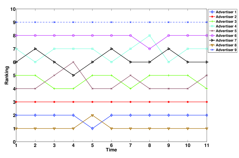
Figure 3: Evolution of $\bar{\sigma}^{u}$ produced by the algorithm for all advertisers.

In Fig. 4, we show the number of adjustments of the ad-quality scores needed for each time instance. We compare two cases in this graph. Case 1: $\epsilon_{q}\sim\mathcal{N}(0,36)$, $\epsilon_{s}\sim\mathcal{N}(0,25)$, $\epsilon_{v}\sim\mathcal{N}(0,0.1)$; Case 2: $\epsilon_{q}\sim\mathcal{N}(0,100)$, let $\epsilon_{s}\sim\mathcal{N}(0,64)$, $\epsilon_{v}\sim\mathcal{N}(0,1)$. It is clear that the parameters of Case 2 are much more volatile than those of case 1. We observe that more volatility in the system parameters results in more adjustments for the algorithm to find the optimal ranking. However, in both cases, once the algorithm finds the social optimal ranking in time instance $1$, the adjustments needed for the algorithm to adapt to the new parameters in the subsequent time instances are small.

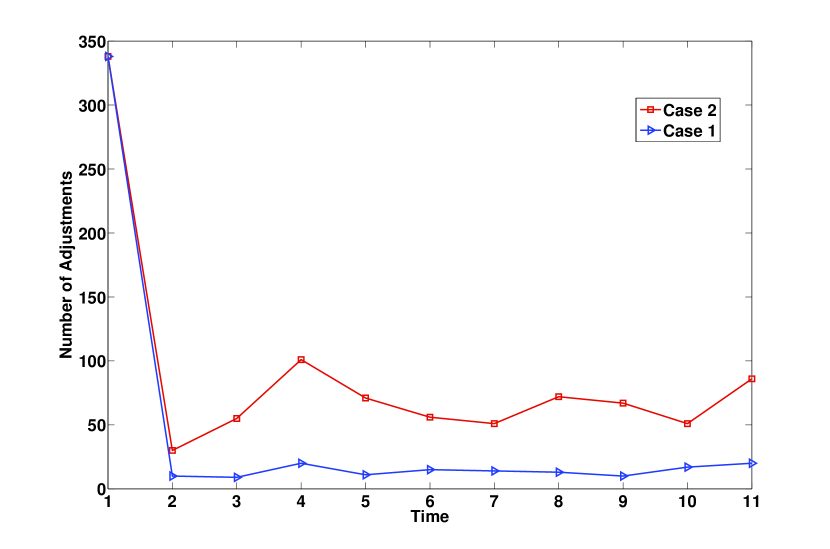
Figure 4: The number of score adjustments needed for each perturbation of the system parameters.

5.3 8-Slot Auction with Modified Click-Through Rate Model

We first describe a modified click-through rate model that takes into consideration the effect relative position between direct competitors on the click-through rates. We assume that among the 9 advertisers, some of them are direct competitors in selling the same type of product (we call them “Group 1 Advertisers"), while the rest of them are not in direct competition with any of the other advertisers (we call them “Group 2 Advertisers"). An example for this situation in reality is that when we search "EOS Camera" on www.goole.com, 6 of the sponsored ads are related to the web sites that sells new Canon EOS cameras; 1 of them sells refurbished EOS cameras, and 1 of them sells magazines relate to Canon EOS cameras. We further assume that there are a fixed number of people that will only click on Group 1 adds (we call them “Group 1 Users"), and they click on each ad $i$ in Group 1 with a probability proportional to $q_{i}s_{i}$. Assume there are a fixed number of people that might click on any of the ads shown, with a probability proportional to each ad’s $q_{i}s_{i}$ . Based on this click-through rate model, the swap of the positions of any two advertisers will result in the change of click-through rate of all other advertisers and our algorithm can no longer guarantee a social optimal ranking every time.

We set the number of Group 1 and Group 2 Advertisers to be $6$ and $3$, respectively; set the number of Group 1 and Group 2 Users to be $400$ and $200$, respectively. We ran the algorithm on $100$ auctions based on the modified click-through rate model with randomly generated parameters $(v,~{}q,~{}e)$. We have obtained a $91.6\%$ averaged ratio of $\Pi_{se}(\bar{\sigma})$ and $\Pi_{se}(\sigma^{\ast})$ for all runs, with a standard deviation of $0.0549$. Although it is less than the averaged ratio we get from the product click-through rate model (almost always larger than $99\%$), it can be seen as a reasonably satisfactory result.

5.4 Efficiency of the Algorithm

The proof of Theorem 3 shows that the optimal rank searching module in the proposed algorithm takes $O\left(N^{2}\right)$ total number of ad-quality score adjustments before the algorithm terminates. While the number of score adjustments in the value revealing module depends on the initial scoring and increment size of the score adjustment, it is polynomial in terms of the input size $v_{i}q_{i}$, for $i=1,...,N$.   The biggest uncertainty that affects the efficiency of the algorithm comes from the function $NE\left(\cdot\right)$. In practice, in order for the revenue to stabilize to determine whether a swap of the neighboring advertisers is profitable, it is required that every time after the scoring profile is adjusted, the advertisers form a certain bidding equilibrium. We argue that over time, the advertisers are likely to learn all relevant information to make an equilibrium decision. Furthermore, this equilibrium does not necessarily need to be an NE and therefore does not require each advertiser to have complete information about others’ behavior. In our implementation with complete information assumption, the algorithm finds the NEs very quickly.

6 Conclusions and discussions

1. The proposed algorithm does not involve any functionality that can not be implemented by the search engines.

2. The proposed algorithm does not involve any estimation of the click-through rates but is solely driven by the total revenue generated which can be observed directly by the search engine. In order for the revenue to stabilize, it is required that every time after the scoring profile is adjusted the advertisers form a certain bidding equilibrium. This equilibrium does not necessarily need to be an NE and therefore does not require each advertiser to have complete information about others’ behavior.

3. Both our theoretical and empirical analysis shows that the search engine can extract almost all the surpluses from the advertisers, given that there are more advertisers than slots and the values of the advertisers can be accurately estimated. Though in reality some of the arguments and assumptions in the model may not hold, our analysis demystifies what a revenue-maximizing scoring strategy for the search engine should look like. Specifically, it first needs to get close to an equalizing scoring profile which solely depends on the estimation of advertisers’ values. Then by making infinitesimal differences between advertisers’ ranking scores, the ranking should be made in the order of the product of the ad-quality specific factor and the advertiser’s value. This is fully consistent with what search engines interpret the ad-quality score. For example, according Google AdWords, the “Quality Score is based on: 1) The historical CTR of the ad on this and similar sites; 2) The quality of your landing page".

4. The theoretical and empirical analysis shown in this paper implies that in a monopoly market where advertisers do not have a choice of other search engines, the monopoly search engine can abuse its power by maximally extracting the surpluses from the advertisers. There are concerns that “… since the ad quality factor is under the search engine’s control, it gives the search engine nearly unlimited power to affect the actual ordering of the advertisers for a given set of bids" [5]. However, to our knowledge, no previous literature has studied theoretically and empirically how far this “unlimited power" can go for a monopoly search engine. The analysis in this paper may lead to new ways of identifying the abusage of a search engine’s monopoly power in charging the advertisers. For example, we can check whether the “ad-quality scores" do reflect the relative qualities in the ads as they claimed to be or they are merely manipulating tools used by the search engine to extract as much surpluses as possible from the advertisers.

References

- [1] H. R. Varian, “Online ad auctions,” Manuscript in preparation, UC Berkerly and Google, 2009.
- [2] B. Edelman, M. Ostrovsky, and M. Schwarz, “Internet advertising and the generalized second-price auction: Selling billions of dollars worth of keywords,” American Economic Review, vol. 97, no. 1, pp. 242–259.
- [3] H. R. Varian, “Position auctions,” International Journal of Industrial Organization, vol. 25, pp. 1163–1178, 2007.
- [4] S. Lahaieh, “An analysis of alternative slot auction designs for sponsored search,” in Proceedings of the 7th ACM conference on Electronic Commerce.
- [5] D. Easley and J. Kleinberg, “Networks, crowds, and markets: Reasoning about a highly connected world,” Cambridge University Press., 2010.