The Fast Cauchy Transform and Faster Robust Linear Regression

Abstract

We provide fast algorithms for overconstrained $\ell_{p}$ regression and related problems: for an $n\times d$ input matrix $A$ and vector $b\in\R^{n}$, in $O(nd\log n)$ time we reduce the problem $\min_{x\in\R^{d}}{\|Ax-b\|}_{p}$ to the same problem with input matrix $\tilde{A}$ of dimension $s\times d$ and corresponding $\tilde{b}$ of dimension $s\times 1$. Here, $\tilde{A}$ and $\tilde{b}$ are a coreset for the problem, consisting of sampled and rescaled rows of $A$ and $b$; and $s$ is independent of $n$ and polynomial in $d$. Our results improve on the best previous algorithms when $n\gg d$, for all $p\in[1,\infty)$ except $p=2$; in particular, they improve the $O(nd^{1.376+})$ running time of Sohler and Woodruff (STOC, 2011) for $p=1$, that uses asymptotically fast matrix multiplication, and the $O(nd^{5}\log n)$ time of Dasgupta et al. (SICOMP, 2009) for general $p$, that uses ellipsoidal rounding. We also provide a suite of improved results for finding well-conditioned bases via ellipsoidal rounding, illustrating tradeoffs between running time and conditioning quality, including a one-pass conditioning algorithm for general $\ell_{p}$ problems.

To complement this theory, we provide a detailed empirical evaluation of implementations of our algorithms for $p=1$, comparing them with several related algorithms. Among other things, our empirical results clearly show that, in the asymptotic regime, the theory is a very good guide to the practical performance of these algorithms. Our algorithms use our faster constructions of well-conditioned bases for $\ell_{p}$ spaces and, for $p=1$, a fast subspace embedding of independent interest that we call the Fast Cauchy Transform: a distribution over matrices $\Pi:\R^{n}\mapsto\R^{O(d\log d)}$, found obliviously to $A$, that approximately preserves the $\ell_{1}$ norms: that is, with large probability, simultaneously for all $x$, ${\|Ax\|}_{1}\approx{\|\Pi Ax\|}_{1}$, with distortion $O(d^{2+\eta})$, for an arbitrarily small constant $\eta>0$; and, moreover, $\Pi A$ can be computed in $O(nd\log d)$ time. The techniques underlying our Fast Cauchy Transform include fast Johnson-Lindenstrauss transforms, low-coherence matrices, and rescaling by Cauchy random variables.

1 Introduction

Random sampling, random projection, and other embedding methods have proven to be very useful in recent years in the development of improved worst-case algorithms for a range of linear algebra problems. For example, Gaussian random projections provide low-distortion subspace embeddings in the $\ell_{2}$ norm, mapping an arbitrary $d$-dimensional subspace in $\R^{n}$ into a $d$-dimensional subspace in $\R^{r}$, with $r=O(d)$, and distorting the $\ell_{2}$ norm of each vector in the subspace by at most a constant factor. Importantly for many applications, the embedding is oblivious in the sense that it is implemented by a linear mapping chosen from a distribution on mappings that is independent of the input subspace. Such low-distortion embeddings can be used to speed up various geometric algorithms, if they can be computed sufficiently quickly. As an example, the Fast Johnson Lindenstrauss transform (FJLT) is one such embedding; the FJLT is computable in $O(n\log d)$ time, using a variant of the fast Hadamard transform [1]. Among other things, use of the FJLT leads to faster algorithms for constructing orthonormal bases, $\ell_{2}$ regression, and $\ell_{2}$ subspace approximation, which in turn lead to faster algorithms for a range of related problems including low-rank matrix approximation [12, 20, 10].

In this paper, we use $\ell_{1}$ and $\ell_{p}$ extensions of these methods to provide faster algorithms for the classical $\ell_{p}$ regression problem and several other related problems. Recall the overconstrained $\ell_{p}$ regression problem.

Definition 1.

Given a matrix $A\in\mathbb{R}^{n\times d}$, with $n>d$, a vector $b\in\mathbb{R}^{n}$, and a norm $\|\cdot\|_{p}$, the $\ell_{p}$ regression problem is to find an optimal solution to:

$$\min_{x\in\mathbb{R}^{d}}\|Ax-b\|_{p}.$$ (1)

In this paper, we are most interested in the case $p=1$, although many of our results hold more generally, and so we state several of our results for general $p$. The $\ell_{1}$ regression problem, also known as the Least Absolute Deviations or Least Absolute Errors problem, is especially of interest as a more robust alternative to the $\ell_{2}$ regression or Least Squares Approximation problem.

It is well-known that for $p\geq 1$, the $\ell_{p}$ regression problem is a convex optimization problem; and for $p=1$ and $p=\infty$, it is an instance of linear programming. Recent work has focused on using sampling, projection, and other embedding methods to solve these problems more quickly than with general convex programming or linear programming methods. Most relevant for our work is the work of Clarkson [6] on solving the $\ell_{1}$ regression problem with subgradient and sampling methods; the work of Dasgupta et al. [7] on using well-conditioned bases and subspace-preserving sampling algorithms to solve general $\ell_{p}$ regression problems; and the work of Sohler and Woodruff [24] on using the Cauchy Transform to obtain improved $\ell_{1}$ embeddings, thereby leading to improved algorithms for the $\ell_{1}$ regression problem. The Cauchy Transform of [24] provides low-distortion embeddings for the $\ell_{1}$ norm, and thus it is an $\ell_{1}$ analog of the Gaussian projection for $\ell_{2}$. It consists of a dense matrix of Cauchy random variables, and so it is “slow” to apply to an arbitrary matrix $A$; but since it provides the first analog of the Johnson-Lindenstrauss embedding for the $\ell_{1}$ norm, it can be used to speed up randomized algorithms for problems such as $\ell_{1}$ regression and $\ell_{1}$ subspace approximation [24].

In this paper, we provide fast algorithms for overconstrained $\ell_{p}$ regression and several related problems. Our algorithms use our faster constructions of well-conditioned bases for $\ell_{p}$ spaces; and, for $p=1$, our algorithms use a fast subspace embedding of independent interest that we call the Fast Cauchy Transform (FCT). We also provide a detailed empirical evaluation of the FCT and its use at computing $\ell_{1}$ well-conditioned bases and solving $\ell_{1}$ regression problems.

The FCT is our main technical result, and it is essentially an $\ell_{1}$ analog of the FJLT. The FCT can be represented by a distribution over matrices $\Pi:\R^{n}\mapsto\R^{O(d\log d)}$, found obliviously to $A$ (in the sense that its construction does not depend on any information in $A$), that approximately preserves the $\ell_{1}$ norms of all vectors in $\{Ax\mid x\in\R^{d}\}$. That is, with large probability, simultaneously for all $x$, ${\|Ax\|}_{1}\approx{\|\Pi Ax\|}_{1}$, with distortion $O(d^{2+\eta}\log d)$, for an arbitrarily small constant $\eta>0$; (see Theorem 2); and, moreover, $\Pi A$ can be computed in $O(nd\log d)$ time. We actually provide two related constructions of the FCT (see Theorems 1 and 2). The techniques underlying our FCTs include FJLTs, low-coherence matrices, and rescaling by Cauchy random variables.

Our main application of the FCT embedding is to constructing the current fastest algorithm for computing a well-conditioned basis for $\ell_{1}$ (see Theorem 3). Such a basis is an analog for the $\ell_{1}$ norm of what an orthonormal basis is for the $\ell_{2}$ norm, and our result improves the result in [24]. We also provide a generalization of this result to constructing $\ell_{p}$ well-conditioned bases (see Theorem 10). The main application for well-conditioned bases is to regression: if the rows of $A$ are sampled according to probabilities derived from the norms of the rows of such a basis, the resulting sample of rows (and corresponding entries of $b$) are with high probability a coreset for the regression problem; see, e.g., [7]. That is, for an $n\times d$ input matrix $A$ and vector $b\in\R^{n}$, we can reduce an $\ell_{p}$ regression problem to another $\ell_{p}$ regression problem with input matrix $\tilde{A}$ of dimension $s\times d$ and corresponding $\tilde{b}$ of dimension $s\times 1$. Here, $\tilde{A}$ and $\tilde{b}$ consist of sampled and rescaled rows of $A$ and $b$; and $s$ is independent of $n$ and polynomial in $d$. We point out that our construction uses as a black box an FJLT, which means that any improvement in the running time of the FJLT (for example exploiting the sparsity of $A$) results in a corresponding improvement to the running times of our $\ell_{p}$ regression.

Based on our constructions of well-conditioned bases, we give the fastest known construction of coresets for $\ell_{p}$ regression, for all $p\in[1,\infty)$, except $p=2$. In particular, for $\ell_{1}$ regression, we construct a coreset of size ${1\over\varepsilon^{2}}\operatorname{poly}(d,\log{1\over\varepsilon})$ that achieves a $(1+\varepsilon)$-approximation guarantee (see Theorem 4). Our construction runs in $O(nd\log n)$ time, improving the previous best algorithm of Sohler and Woodruff [24], which has an $O(nd^{1.376+})$ running time. Our extension to finding an $\ell_{p}$ well-conditioned basis also leads to an $O(nd\log n)$ time algorithm for a $(1+\varepsilon)$-approximation to the $\ell_{p}$ regression problem (see Theorem 11), improving the $O(nd^{5}\log n)$ algorithm of Dasgupta et al. [7]. For $p=1$, extensions of our basic methods yield improved algorithms for several related problems. For example, we actually further optimize the running time for $p=1$ to $O(nd\log(\varepsilon^{-1}d\log n))$ (see Theorem 5). In addition, we generalize our $\ell_{1}$ result to solving the multiple regression problem (see Theorem 6); and we use this to give the current fastest algorithm for computing a $(1+\varepsilon)$-approximation for the $\ell_{1}$ subspace approximation problem (see Theorem 7).

In addition to our construction of $\ell_{p}$ well-conditioned bases (see Theorem 10) and their use in providing a $(1+\varepsilon)$-approximation to the $\ell_{p}$ regression problem (see Theorem 11), we also provide a suite of improved results for finding well-conditioned bases via ellipsoidal rounding for general $\ell_{p}$ problems, illustrating tradeoffs between running time and conditioning quality. These methods complement the FCT-based methods in the sense that the FCT may be viewed as a tool to compute a good basis in an oblivious manner, and the ellipsoid-based methods provide an alternate way to compute a good basis in a data-dependent manner. In particular, we prove that we can obtain an ellipsoidal rounding matrix in at most $O(nd^{3}\log n)$ time that provides a $2d$-rounding (see Theorem 9). This is much faster than the algorithm of Lovász [19] that computes a $(d(d+1))^{1/2}$-rounding in $O(nd^{5}\log n)$ time. We also present an optimized algorithm that uses an FJLT to compute a well-conditioned basis of $A$ in $O(nd\log n)$ time (see Theorem 10). When $p=1$, these $\ell_{p}$ rounding algorithms are competitive with or better than previous algorithms that were developed for $\ell_{1}$.

Finally, we also provide the first empirical evaluation for this class of randomized algorithms. In particular, we provide a detailed evaluation of a numerical implementation of both FCT constructions, and we compare the results with an implementation of the (slow) Cauchy Transform, as well as a Gaussian Transform and an FJLT. These latter two are $\ell_{2}$-based projections. We evaluate the quality of the $\ell_{1}$ well-conditioned basis, the core component in all our geometric algorithms, on a suite of matrices designed to test the limits of these randomized algorithms, and we also evaluate how the method performs in the context of $\ell_{1}$ regression. This latter evaluation includes an implementation on a nearly terabyte-scale problem, where we achieve a $10^{-3}$ relative-error approximation to the optimal solution, a task that was infeasible prior to our work. Among other things, our empirical results clearly show that, in the asymptotic regime, the theory is a very good guide to the practical performance of these algorithms.

Since this paper is long and detailed, we provide here a brief outline. We start in Section 2 with some preliminaries, including several technical results that we will use in our analysis and that are of independent interest. Then, in Section 3, we will present our main technical results for the Fast Cauchy Transform; and in Section 4, we will describe applications of it to $\ell_{1}$ well-conditioned basis construction and $\ell_{1}$ leverage score approximation, to solving the $\ell_{1}$ regression problem, and to solving the $\ell_{1}$ norm subspace approximation problem. Then, in Section 5, we describe extensions of these ideas to general $\ell_{p}$ problems. Section 6 will contain a detailed empirical evaluation of our algorithms for $\ell_{1}$-based problems, including the construction of $\ell_{1}$ well-conditioned bases and both small-scale and large-scale $\ell_{1}$ regression problems. Section 7 will then contain a brief conclusion. For simplicity of presentation, the proofs of our main results have been moved to Appendices A through J.

2 Preliminaries

Let $A\in\R^{n\times d}$ be an $n\times d$ input matrix, where we assume $n\gg d$ and $A$ has full column rank. The task of linear regression is to find a vector $x^{*}\in\R^{d}$ that minimizes ${\|Ax-b\|}$ with respect to $x$, for a given $b\in\R^{n}$ and norm ${\|\cdot\|}$. In this paper, our focus is mostly on the $\ell_{1}$ norm, although we also discuss extensions to $\ell_{p}$, for any $p\geq 1$. Recall that, for $p\in[1,\infty]$, the $\ell_{p}$ norm of a vector $x$ is ${\|x\|}_{p}=\left(\sum_{i}|x_{i}|^{p}\right)^{1/p}$, defined to be $\max_{i}|x_{i}|$ for $p=\infty$. Let $[n]$ denote the set $\{1,2,\ldots,n\}$; and let $A_{(i)}$ and $A^{(j)}$ be the $i$th row vector and $j$th column vector of $A$, respectively. For matrices, we use the Frobenius norm $\mbox{}\left\|A\right\|_{F}^{2}=\sum_{i=1}^{n}\sum_{j=1}^{d}A_{ij}^{2}$, the $\ell_{2}$-operator (or spectral) norm $\mbox{}\left\|A\right\|_{2}=\sup_{\ \mbox{}\left\|x\right\|_{2}=1}\mbox{}\left\|Ax\right\|_{2}$, and the entrywise $\ell_{p}$ norm ${\|X\|}_{p}=(\sum_{i,j}|X_{ij}|^{p})^{1/p}$. (The exception to this is $p=2$, where this notation is used for the spectral norm and the entrywise 2-norm is the Frobenius norm.) Finally, the standard inner product between vectors $x,y$ is $\langle x,y\rangle=x^{T}y$; $e_{i}$ are standard basis vectors of the relevant dimension; $I_{n}$ denotes the $n\times n$ identity matrix; and $c$ refers to a generic constant whose specific value may vary throughout the paper.

Two Useful Tail Inequalities.

The following two Bernstein-type tail inequalities are useful because they give tail bounds without reference to the number of i.i.d. trials. The first bound is due to Maurer [22], and the second is an immediate application of the first.

Lemma 1 ([22]).

Let $X_{i}\geq 0$ be independent random variables with $\sum_{i}\hbox{\bf{E}}[X_{i}^{2}]<\infty$, and define $X=\sum_{i}X_{i}$. Then, for any $t>0$,

$$\hbox{\bf{Pr}}[X\leq\hbox{\bf{E}}[X]-t]\leq\operatorname{exp}\left({-t^{2}\over 2\sum_{i}\hbox{\bf{E}}[X_{i}^{2}]}\right).$$

Lemma 2.

Let $x_{i}$ be i.i.d. Bernoulli random variables with probability $p$, and let $X=\sum_{i\in[n]}\xi_{i}x_{i}$, where $\xi_{i}\geq 0$, with $\sum_{i\in[n]}\xi_{i}=\xi$ and $\sum_{i\in[n]}\xi_{i}^{2}\leq\xi^{2}/\beta^{2}$. Then, for any $t>0$,

$$\hbox{\bf{Pr}}[X\geq\xi(p+t)]\leq\operatorname{exp}\left(-{\beta^{2}t^{2}\over 2(1-p)}\right).$$

Proof.

The proof is a straightforward application of Lemma 1 to $Z=\sum_{i\in[n]}\xi_{i}(1-x_{i})$. ∎

Sums of Cauchy Random Variables.

The Cauchy distribution, having density $p(x)={1\over\pi}{1\over 1+x^{2}}$, is the unique $1$-stable distribution. If $C_{1},\ldots,C_{M}$ are independent Cauchys, then $\sum_{i\in[M]}\gamma_{i}C_{i}$ is distributed as a Cauchy scaled by $\gamma=\sum_{i\in[M]}|\gamma_{i}|$. The Cauchy distribution will factor heavily in our discussion, and bounds for sums of Cauchy random variables will be used throughout. We note that the Cauchy distribution has undefined expectation and infinite variance.

The following upper and lower tail inequalities for sums of Cauchy random variables are proved in Appendix A. The proof of Lemma 3 is similar to an argument of Indyk [15], though in that paper the Cauchy random variables are independent. As in that paper, our argument follows by a Markov bound after conditioning on the magnitudes of the Cauchy random variable summands not being too large, so that their conditional expectations are defined. However, in this paper, the Cauchy random variables are dependent, and so after conditioning on a global event, the expectations of the magnitudes need not be the same as after this conditioning in the independent case.

Lemma 4 is a simple application of Lemma 1, while Lemma 5 was shown in [7]; we include the proofs for completeness.

Lemma 3 (Cauchy Upper Tail Inequality).

For $i\in[m]$, let $C_{i}$ be $m$ (not necessarily independent) Cauchy random variables, and $\gamma_{i}>0$ with $\gamma=\sum_{i\in[m]}\gamma_{i}$. Let $X=\sum_{i\in[m]}\gamma_{i}|C_{i}|$. Then, for any $t\geq 1$,

$$\hbox{\bf{Pr}}\left[X>\gamma t\right] \leq {1\over\pi t}\left({\log(1+(2mt)^{2})\over 1-1/(\pi t)}+1\right)={\log(mt)\over t}\left(1+{\textstyle o(1)}\right).$$

Remark. The bound has only logarithmic dependence on the number of Cauchy random variables and does not rely on any independence assumption among the random variables. Even if the Cauchys are independent, one cannot substantially improve on this bound due to the nature of the Cauchy distribution. This is because, for independent Cauchys, $\sum_{i}\gamma_{i}|C_{i}|\geq|\sum_{i}\gamma_{i}C_{i}|$, and the latter sum is itself distributed as a Cauchy scaled by $\gamma$. Hence for independent Cauchys, $\hbox{\bf{Pr}}[X\geq\gamma t]={2\over\pi}\tan^{-1}t=\Omega({1\over t})$.

Lemma 4 (Cauchy Lower Tail Inequality).

For $i\in[r]$, let $C_{i}$ be independent Cauchy random variables, and $\gamma_{i}\geq 0$ with $\gamma=\sum_{i\in[r]}\gamma_{i}$ and $\sum_{i\in[r]}{\gamma_{i}^{2}}\leq\gamma^{2}/\beta^{2}$. Let $X=\sum_{i\in[r]}\gamma_{i}|C_{i}|$. Then, for any $t\geq 0$,

$$\hbox{\bf{Pr}}\left[X\leq\gamma(1-t)\right]\leq\operatorname{exp}\left(-{\beta^{2}t^{2}\over 3}\right).$$

An $\ell_{1}$ Sampling Lemma.

We will also need an “$\ell_{1}$-sampling lemma,” which is an application of Bernstein’s inequality. This lemma bounds how $\ell_{1}$ norms get distorted under sampling according to $\ell_{1}$ probabilities. The proof of this lemma is also given in Appendix A.

Lemma 5 ($\ell_{1}$ Sampling Lemma).

Let $Z\in\R^{n\times k}$ and suppose that for $i\in[n]$, $t_{i}\geq a{\|Z_{(i)}\|}_{1}/{\|Z\|}_{1}$. For $s>0$, define $\hat{p}_{i}=\min\{1,s\cdot t_{i}\}$, and let $D\in\R^{n\times n}$ be a random diagonal matrix with $D_{ii}=1/\hat{p}_{i}$ with probability $\hat{p}_{i}$, and $0$ otherwise. Then, for any (fixed) $x\in\mathbb{R}^{k}$, with probability at least $1-\delta$,

$$(1-\varepsilon){\|Zx\|}_{1}\leq{\|DZx\|}_{1}\leq(1+\varepsilon){\|Zx\|}_{1},$$

where $\displaystyle\delta\leq 2\operatorname{exp}\left({-as\varepsilon^{2}{\|Zx\|}_{1}\over(2+{2\over 3}\varepsilon){\|Z\|}_{1}{\|x\|}_{\infty}}\right).$

3 Main Technical Result: the Fast Cauchy Transform

In this section, we present the Fast Cauchy Transform (FCT), which is an $\ell_{1}$-based analog of the fast Johnson-Lindenstrauss transform (FJLT). We will actually present two related constructions, one based on using a quickly-constructable low-coherence matrix, and one based on using a version of the FJLT. In both cases, these matrices will be rescaled by Cauchy random variables (hence the name Fast Cauchy Transform). We will also state our main results, Theorems 1 and 2, which provides running time and quality-of-approximation guarantees for these two FCT embeddings.

3.1 FCT1 Construction: via a Low-coherence Matrix

This FCT construction first preprocesses by a deterministic low-coherence “spreading matrix,” then rescales by Cauchy random variables, and finally samples linear combinations of the rows. Let $\delta\in(0,1]$ be a parameter governing the failure probability of our algorithm. Then, we construct $\Pi_{1}$ as

$$\Pi_{1}\equiv 4BC\tilde{H},$$

where:

$B\in\R^{r_{1}\times 2n}$ has each column chosen independently and uniformly from the $r_{1}$ standard basis vectors for $\R^{r_{1}}$; we will set the parameter $r_{1}=\alpha d\log{d\over\delta}$, where $\delta$ controls the probability that our algorithms fail and $\alpha$ is a suitably large constant;

$C\in\R^{2n\times 2n}$ is a diagonal matrix with diagonal entries chosen independently from a Cauchy distribution; and

$\tilde{H}\in\R^{2n\times n}$ is a block-diagonal matrix comprised of $n/s$ blocks along the diagonal. Each block is the $2s\times s$ matrix $G_{s}\equiv\left[\begin{smallmatrix}H_{s}\\ I_{s}\end{smallmatrix}\right]$, where $I_{s}$ is the $s\times s$ identity matrix, and $H_{s}$ is the normalized Hadamard matrix. We will set $s=r_{1}^{6}$. (Here, for simplicity, we assume $s$ is a power of two and $n/s$ is an integer.)

$$\tilde{H}\equiv\left[\begin{matrix}G_{s}&&\\ &G_{s}&&\\ &&\ddots&\\ &&&G_{s}\\ \end{matrix}\right]$$

(For completeness, we remind the reader that the (non-normalized) $n\times n$ matrix of the Hadamard transform $H_{n}$ may be defined recursively as follows:

$$H_{n}=\left[\begin{array}[]{cc}H_{n/2}&H_{n/2}\\ H_{n/2}&-H_{n/2}\end{array}\right],\quad\mbox{with}\quad H_{2}=\left[\begin{array}[]{cc}+1&+1\\ +1&-1\end{array}\right].$$

The $n\times n$ normalized matrix of the Hadamard transform is then equal to ${1\over\sqrt{n}}H_{n}$; hereafter, we will denote this normalized matrix by $H_{n}$.) Heuristically, the effect of $\tilde{H}$ in the above FCT construction is to spread the weight of a vector, so that $\tilde{H}y$ has many entries that are not too small. (This is discussed in Lemma 7 in the proof of Theorem 1 below.) This means that the vector $C\tilde{H}y$ comprises Cauchy random variables with scale factors that are not too small; and finally these variables are summed up by $B$, yielding a vector $BC\tilde{H}y$, whose $\ell_{1}$ norm won’t be too small relative to $\lVert y\rVert_{1}$. For this version of the FCT, we have the following theorem. The proof of this theorem may be found in Appendix B.

Theorem 1 (Fast Cauchy Transform (FCT1)).

There is a distribution (given by the above construction) over matrices $\Pi_{1}\in\R^{r_{1}\times n}$, with $r_{1}=O(d\log d+d\log{1\over\delta})$, such that for an arbitrary (but fixed) $A\in\R^{n\times d}$, and for all $x\in\R^{d}$, the inequalities

$${\|Ax\|}_{1}\leq{\|\Pi_{1}Ax\|}_{1}\leq\kappa{\|Ax\|}_{1}$$ (2)

hold with probability $1-\delta$, where

$$\kappa=O\left({d\sqrt{s}\over\delta}\log(r_{1}d)\right).$$

Further, for any $y\in\R^{n}$, the product $\Pi_{1}y$ can be computed in $O(n\log r_{1})$ time.

Setting $\delta$ to a small constant, since $\sqrt{s}=r_{1}^{3}$ and $r_{1}=O(d\log d)$, it follows that $\kappa=O(d^{4}\log^{4}d)$ in the above theorem.

Remark.

The existence of such a $\Pi_{1}$ satisfying bounds of the form (2) was established by Sohler and Woodruff [24]. Here, our contribution is to show that $\Pi_{1}$ can be factored into structured matrices so that the product $\Pi_{1}A$ can be computed in $O(nd\log d)$ time. We also remark that, in additional theoretical bounds provided by the FJLT, high-quality numerical implementations of variants of the Hadamard transform exist, which is an additional plus for our empirical evaluations of Theorem 1 and Theorem 2.

Remark.

Our proof of this theorem uses a tail bound for ${\|Bg\|}_{2}^{2}$ in terms of ${\|g\|}_{2}$ and ${\|g\|}_{1}$, where $g$ is any positive vector in $\R^{n}$, and $B$ is the matrix used in our FCT construction. ${\|Bg\|}_{2}^{2}=\sum_{j}{\gamma_{j}^{2}}$ where $\gamma_{j}=\sum_{i}B_{ji}g_{i}$ are anti-correlated random variables. To get concentration, we independently bounded $\gamma_{j}^{2}$ in our proof which required $s=r_{1}^{6}$ to obtain the high probability result; this resulted in the bound $\kappa=O(d^{4}\log^{4}d)$.

3.2 FCT2 Construction: via a Fast Johnson-Lindenstrauss Transform

This FCT construction first preprocesses by a FJLT and then rescales by Cauchy random variables. Recall that $\delta\in(0,1]$ is a parameter governing the failure probability of our algorithm; and let $\eta>0$ be a generic arbitrarily small positive constant (whose value may change from one formula to another). Let $r_{1}=c\cdot d\log{d\over\delta}$, $s=c^{\prime}\cdot(d+\log{n\over\delta})$, and $t=s^{2+\eta}$, where the parameters $c,c^{\prime}>0$ are appropriately large constants. Then, we construct $\Pi_{1}\in\R^{r_{1}\times n}$ as

$$\Pi_{1}\equiv{8\over r_{1}}\sqrt{{\pi t\over 2s}}\cdot C\tilde{H},$$

where:

$C\in\R^{r_{1}\times ns/t}$ is a matrix of independent Cauchy random variables; and

$\tilde{H}\in\R^{ns/t\times n}$ is a block-diagonal matrix comprising $n/t$ blocks along the diagonal. Each block is the $s\times t$ Fast Johnson-Lindenstrauss matrix $G$. (The important property that $G$ must satisfy is given by Lemmas 9 and 10 in the proofs below.) Here, for simplicity, we assume that $n/t$ is an integer.

$$\tilde{H}\equiv\left[\begin{matrix}G&&\\ &G&&\\ &&\ddots&\\ &&&G\\ \end{matrix}\right].$$

Informally, the matrix $\tilde{H}$ reduces the dimensionality of the input space by a very small amount such that the “slow” Cauchy Transform $C$ of [24] can be applied in the allotted time. Then, since we are ultimately multiplying by $C$, the results of [24] still hold; but since the dimensionality is slightly reduced, the running time is improved. For this version of the FCT, we have the following theorem. The proof of this theorem may be found in Appendix C.

Theorem 2 (Fast Cauchy Transform (FCT2)).

There is a distribution (given by the above construction) over matrices $\Pi_{1}\in\R^{r_{1}\times n}$, with $r_{1}=O(d\log{d\over\delta})$, such that for arbitrary (but fixed) $A\in\R^{n\times d}$, and for all $x\in\R^{d}$, the inequalities

$${\|Ax\|}_{1}\leq{\|\Pi_{1}Ax\|}_{1}\leq\kappa{\|Ax\|}_{1}$$

hold with probability $1-\delta$, where $\kappa=O({d\over\delta}(d+\log{n\over\delta})^{1+\eta}\log d)$. Further, for any $y\in\R^{n}$, the product $\Pi_{1}y$ can be computed in $O(n\log{d\over\delta})$ time.

Setting $\delta$ to be a small constant and for $\log n<d$, $r_{1}=O(d\log d)$, $\kappa=O(d^{2+\eta}\log d)$ and $\Pi_{1}A$ can be computed in $O(nd\log d)$ time. Thus, we have a fast linear oblivious mapping from from $\ell_{1}^{n}\mapsto\ell_{1}^{O(d\log d)}$ that has distortion $O(d^{2+\eta}\log d)$ on any (fixed) $d$-dimensional subspace of $\R^{n}$.

Remark. For $\log n<d$, FCT2 gives a better dependence of the distortion on $d$, but more generally FCT2 has a dependence on $\log n$. This dependence arises because the random FJLT matrix does not give a deterministic guarantee for spreading out a vector whereas the low coherence matrix used in FCT1 does give a deterministic guarantee. This means that in using the union bound, we need to overcome a factor of $n$.

Remark. The requirement $t\geq s^{2+\eta}$ is set by the restriction in Lemma 9 in the proof of Theorem 2. In the bound of Theorem 2, $\kappa=\kappa^{\prime}\sqrt{t}$, where $\kappa^{\prime}=O(d\log(r_{1}d))$ arises from Theorem 12, which originally appeared in [24]. If a stronger version of Lemma 9 can be proved that relaxes the restriction $t\geq s^{2+\eta}$, then correspondingly the bound of Theorem 2 will improve.

Remark. This second construction has the benefit of being easily extended to constructing well-conditioned bases of $\ell_{p}$, for $p>1$; see Section 5.

4 Algorithmic Applications in $\ell_{1}$ of the FCT

In this section, we describe three related applications of the FCT to $\ell_{1}$-based problems. The first is to the fast construction of an $\ell_{1}$ well-conditioned basis and the fast approximation of $\ell_{1}$ leverage scores; the second is a fast algorithm for the least absolute deviations or $\ell_{1}$ regression problem; and the third is to a fast algorithm for the $\ell_{1}$ norm subspace approximation problem.

4.1 Fast Construction of an $\ell_{1}$ Well-conditioned Basis and $\ell_{1}$ Leverage Scores

We start with the following definition, adapted from [7], of a basis that is “good” for the $\ell_{1}$ norm in a manner that is analogous to how an orthogonal matrix is “good” for the $\ell_{2}$ norm.

Definition 2 ($\ell_{1}$ Well-conditioned Basis (adapted from [7])).

A basis $U$ for the range of $A$ is $(\alpha,\beta)$-conditioned if ${\|U\|}_{1}\leq\alpha$ and for all $x\in\R^{d}$, ${\|x\|}_{\infty}\leq\beta{\|Ux\|}_{1}$. We will say that $U$ is well-conditioned if $\alpha$ and $\beta$ are low-degree polynomials in $d$, independent of $n$.

Remark. An Auerbach basis for $A$ is $(d,1)$-conditioned, and thus we know that there exist well-conditioned bases for $\ell_{1}$. More generally, well-conditioned bases can be defined in any $\ell_{p}$ norm, using the notion of a dual norm $\ell_{p}^{*}$, and these have proven important for solving $\ell_{p}$ regression problems [7]. Our focus in this section is the $\ell_{1}$ norm, for which the dual norm is the $\ell_{\infty}$ norm, but in Section 5 we will return to a discussion of extensions to the $\ell_{p}$ norm.

Our main algorithm for constructing an $\ell_{1}$ well-conditioned basis, FastL1Basis, is summarized in Figure 1. This algorithm was originally presented in [24], and our main contribution here is to improve its running time. We note that in step 3, we do not explicitly compute the product of $A$ and $R^{-1}$, but rather just return $A$ and $R^{-1}$ with the promise that $AR^{-1}$ is well-conditioned. The leading order term in our running time to compute $R^{-1}$ is $O(nd\log d)$, while in  [24] it is $O(nd^{2})$, or with fast matrix multiplication, $O(nd^{1.376})$.

Given an $n\times d$ matrix $A$, let $\Pi_{1}\in\R^{r_{1}\times n}$ be any projection matrix such that for any $x\in\R^{d}$,

$${\|Ax\|}_{1}\leq{\|\Pi_{1}Ax\|}_{1}\leq\kappa{\|Ax\|}_{1}.$$ (3)

For example, it could be constructed with either of the FCT constructions described in Section 3, or with the “slow” Cauchy Transform of [24], or via some other means. After computing the matrix $\Pi_{1}$, the FastL1Basis algorithm of Figure 1 consists of the following steps: construct $\Pi_{1}A$ and an $R$ such that $\Pi_{1}A=QR$, where $Q$ has orthonormal columns (for example using a QR-factorization of $\Pi_{1}A$); and then return $U=AR^{-1}=A(Q^{T}\Pi_{1}A)^{-1}$.

FastL1Basis$(A)$: 1:  Let $\Pi_{1}$ be an $r_{1}\times n$ matrix satisfying (3), e.g., as constructed with one of the FCTs of Section 3. 2:  Compute $\Pi_{1}A\in\mathbb{R}^{r_{1}\times d}$ and its QR-factorization: $\Pi_{1}A=QR$, where $Q$ is an orthogonal matrix, i.e., $Q^{T}Q=I$. 3:  Return $U=AR^{-1}=A(Q^{T}\Pi_{1}A)^{-1}$

Figure 1: Our main algorithm for the fast construction of an $\ell_{1}$ well-conditioned basis of an $n\times d$ matrix $A$. Note the structural similarities with the algorithm of [10] for computing quickly approximations to the $\ell_{2}$ leverage scores and an $\ell_{2}$ well-conditioned basis.

The next theorem and its corollary are our main results for the FastL1Basis algorithm; and this theorem follows by combining our Theorem 2 with Theorems 9 and 10 of [24]. The proof of this theorem may be found in Appendix D.

Theorem 3 (Fast $\ell_{1}$ Well-conditioned Basis).

For any $A\in\R^{n\times d}$, the basis $U=A{R^{-1}}$ constructed by FastL1Basis$(A)$ of Figure 1 using any $\Pi_{1}$ satisfying (3) is a $(d\sqrt{r_{1}},\kappa)$-conditioned basis for the range of $A$.

Corollary 1.

If $\Pi_{1}$ is obtained from the FCT2 construction of Theorem 2, then the resulting $U$ is an $(\alpha,\beta)$-conditioned basis for $A$, with $\alpha=O(d^{3/2}\log^{1/2}d)$ and $\beta=O(d^{2+\eta}\log d)$, with probability $1-\delta$. The time to compute the change of basis matrix ${R^{-1}}$ is $O(nd\log d+d^{3}\log d)$, assuming $\log n=O(d)$ and $\delta>0$ is a fixed constant.

Remark. Our constructions that result in $\Pi_{1}$ satisfying (3) do not require that $A\in\R^{n\times d}$; they only require that $A$ have rank $d$, and so can be applied to any $A\in\R^{n\times m}$ having rank $d$. In this case, a small modification is needed in the construction of $U$, because $R\in\R^{d\times m}$, and so we need to use $R^{\dagger}$ instead of $R^{-1}$. The running time will involve terms with $m$. This can be improved by processing $A$ quickly into a smaller matrix by sampling columns so that the range is preserved (as in [24]), which we do not discuss further.

The notion of a well-conditioned basis plays an important role in our subsequent algorithms. Basically, the reason is that these algorithms compute approximate answers to the problems of interest (either the $\ell_{1}$ regression problem or the $\ell_{1}$ subspace approximation problem) by using information in that basis to construct a nonuniform importance sampling distribution with which to randomly sample. This motivates the following definition.

Definition 3 ($\ell_{1}$ Leverage Scores).

Given a well-conditioned basis $U$ for the range of $A$, let the $n$-dimensional vector $\tilde{\lambda}$, with elements defined as $\tilde{\lambda}_{i}=||U_{(i)}||_{1},$ be the $\ell_{1}$ leverage scores of $A$.

Remark. The name $\ell_{1}$ leverage score is by analogy with the $\ell_{2}$ leverage scores, which are important in random sampling algorithms for $\ell_{2}$ regression and low-rank matrix approximation [21, 20, 10]. As with $\ell_{2}$ regression and low-rank matrix approximation, our result for $\ell_{1}$ regression and $\ell_{1}$ subspace approximation will ultimately follow from the ability to approximate these scores quickly. Note, though, that these $\ell_{1}$-based scores are not well-defined for a given matrix $A$, in the sense that the $\ell_{1}$ norm is not rotationally invariant, and thus depending on the basis that is chosen, these scores can differ by factors that depend on low-degree polynomials in $d$. This contrasts with $\ell_{2}$, since for $\ell_{2}$ any orthogonal matrix spanning a given subspace leads to the same $\ell_{2}$ leverage scores. We will tolerate this ambiguity since these $\ell_{1}$ leverage scores will be used to construct an importance sampling distribution, and thus up to low-degree polynomial factors in $d$, which our analysis will take into account, it will not matter.

4.2 Fast $\ell_{1}$ Regression

Here, we consider the $\ell_{1}$ regression problem, also known as the least absolute deviations problem, the goal of which is to minimize the $\ell_{1}$ norm of the residual vector $Ax-b$. That is, given as input a design matrix $A\in\mathbb{R}^{n\times d}$, with $n>d$, and a response or target vector $b\in\mathbb{R}^{n}$, compute

$$\min_{x\in\mathbb{R}^{d}}||Ax-b||_{1},$$ (4)

and an $x^{*}$ achieving this minimum. We start with our main algorithm and theorem for this problem; and we then describe how a somewhat more sophisticated version of the algorithm yields improved running time bounds.

4.2.1 Main Algorithm for Fast $\ell_{1}$ Regression

Prior work has shown that there is a diagonal sampling matrix $D$ with a small number of nonzero entries so that $\hat{x}=\operatorname{argmin}\nolimits_{x\in\R^{d}}\lVert D(Ax-b)\rVert_{1}$ satisfies

$$\lVert A\hat{x}-b\rVert_{1}\leq(1+\varepsilon)\lVert Ax^{*}-b\rVert_{1},$$

where $x^{*}$ is an optimal solution for the minimization in (4); see [7, 24]. The matrix $D$ can be found by sampling its diagonal entries independently according to a set of probabilities $p_{i}$ that are proportional to the $\ell_{1}$ leverage scores of $A$. Here, we give a fast algorithm to compute estimates $\hat{p}_{i}$ of these probabilities. This permits us to develop an improved algorithm for $\ell_{1}$ regression and to construct efficiently a small coreset for an arbitrary $\ell_{1}$ regression problem.

In more detail, Figure 2 presents the FastCauchyRegression algorithm, which we summarize here. Let $X=\left[\begin{matrix}A&-b\end{matrix}\right]$. First, a matrix $\Pi_{1}$ satisfying (3) is used to reduce the dimensionality of $X$ to $\Pi_{1}X$ and to obtain the orthogonalizer $R^{-1}$. Let $U=X{R^{-1}}$ be the resulting well-conditioned basis for the range of $X$. The probabilities we use to sample rows are essentially the row-norms of $U$. However, to compute $XR^{-1}$ explicitly takes $O(nd^{2})$ time, which is already too costly, and so we need to estimate ${\|U_{(i)}\|}_{1}$ without explicitly computing $U$. To construct these probabilities quickly, we use a second random projection $\Pi_{2}$—on the right. This second projection allows us to estimate the norms of the rows of $XR^{-1}$ efficiently to within relative error (which is all we need) using the median of $r_{2}$ independent Cauchy’s, each scaled by $||U_{(i)}||_{1}$. (Note that this is similar to what was done in [10] to approximate the $\ell_{2}$ leverage scores of an input matrix.) These probabilities are then used to construct a carefully down-sampled (and rescaled) problem, the solution to which will give us our $(1+\varepsilon)$ approximation to the original problem.

FastCauchyRegression$(A,b)$: 1:  Let $X=\left[\begin{matrix}A&-b\end{matrix}\right]\in\R^{n\times(d+k)}$ and construct $\Pi_{1}$, an $r_{1}\times n$ matrix satisfying (3) with $A$ replaced by $X$. (If $b$ is a vector then $k=1$.) 2:  Compute $X^{\prime}=\Pi_{1}X\in\mathbb{R}^{r_{1}\times(d+k)}$ and its QR factorization, $\Pi_{1}X=QR$. (Note that $\Pi_{1}XR^{-1}$ has orthonormal columns.) 3:  Let $\Pi_{2}\in\R^{(d+k)\times r_{2}}$ be a matrix of independent Cauchys, with $r_{2}=15\log{2n\over\delta}$. 4:  Let $U=X{R^{-1}}$ and construct $\Lambda=U\Pi_{2}\in\R^{n\times r_{2}}$. 5:  For $i\in[n]$, compute $\lambda_{i}=\operatorname{median}_{j\in[r_{2}]}|\Lambda_{ij}|.$ 6:  For $i\in[n]$ and $s={63\kappa(d+k)\sqrt{r_{1}}\over\varepsilon^{2}}\left((d+k)\log{24\kappa(d+k)\sqrt{r_{1}}\over\varepsilon}+\log{2\over\delta}\right)$, compute probabilities $$\hat{p}_{i}=\min\left\{1,s\cdot{\lambda_{i}\over\sum_{i\in[n]}\lambda_{i}}\right\}.$$ 7:  Let $D\in\R^{n\times n}$ be diagonal with independent entries: $D_{ii}=\begin{cases}{1\over\hat{p}_{i}}&\text{prob. }\hat{p}_{i};\\ 0&\text{prob. }1-\hat{p}_{i}.\end{cases}$ 8:  Return $\hat{x}\in\R^{d}$ that minimizes ${\|DAx-Db\|}_{1}$ w.r.t. $x$ (using linear programming).

Figure 2: Algorithm for solving $\ell_{1}$ regression. Note that in Step 6, we sample rows of $A$ and $b$ so that the expected number of rows sampled is at most $s$. Instead of this independent sampling (without replacement), we could sample exactly $s$ rows independently with replacement according to the probabilities $\hat{p}_{i}=\lambda_{i}/\sum_{i\in[n]}\lambda_{i}$, and all our results continue to hold up to small factors.

The next theorem summarizes our main quality-of-approximation results for the FastCauchyRegression algorithm of Figure 2. It improves the $O(nd^{2}+\operatorname{poly}(d\varepsilon^{-1}\log n))$ algorithm of [24], which in turn improved the result in [7]. (Technically, the running time of [24] is $O(nd^{\omega^{+}-1}+\operatorname{poly}(d\varepsilon^{-1}\log n))$, where $\omega^{+}$ is any constant larger than the exponent for matrix multiplication; for practical purposes, we can set $\omega^{+}=3$.) Our improved running time comes from using the FCT and a simple row-norm estimator for the row-norms of a well-conditioned basis. The proof of this theorem may be found in Appendix E.

Theorem 4 (Fast Cauchy $\ell_{1}$ Regression).

Given are $\varepsilon\in(0,1)$, $\rho>0$, $A\in\R^{n\times d}$ and $b\in\R^{n}$. FastCauchyRegression$(A,b)$ constructs a coreset specified by the diagonal sampling matrix $D$ and a solution vector $\hat{x}\in\R^{d}$ that minimizes the weighted regression objective ${\|D(Ax-b)\|}_{1}$. The solution $\hat{x}$ satisfies, with probability at least $1-{1\over d^{\rho}}$ ($\rho>0$ is a constant),

$${\|A\hat{x}-b\|}_{1}\leq\left({1+\varepsilon\over 1-\varepsilon}\right){\|Ax-b\|}_{1},\qquad\forall x\in\R^{d}.$$

Further, with probability $1-o(1)$, the entire algorithm to construct $\hat{x}$ runs in time

$$O\left(nd\log n+\phi(s,d)\right)=O\left(nd\log n+{\textstyle{1\over\varepsilon^{2}}\operatorname{poly}(d,\log{d\over\varepsilon})}\right),$$

where $\phi(s,d)$ is the time to solve an $\ell_{1}$-regression problem on $s$ vectors in $d$ dimensions, and if FCT2 is used to construct $\Pi_{1}$ then $s=O\left({1\over\varepsilon^{2}}d^{\rho+{9\over 2}+\eta}\log^{{3\over 2}}({d\over\varepsilon})\right)$.

Remarks. Several remarks about our results for the $\ell_{1}$ regression problem are in order.

• Our proof analyzes a more general problem $\min_{x\in{\cal C}}||Xx||_{1}$, where ${\cal C}\subseteq\R^{d}$ is a convex set. In order to get the result, we need to preserve norms under sampling, which is what Lemma 5 allows us to do. We mention that our methods extend with minor changes to $\ell_{p}$ regression, for $p>1$. This is discussed in Section 5.

• A natural extension of our algorithm to matrix-valued right hand sides $b$ gives a $(1+\varepsilon)$ approximation in a similar running time for the $\ell_{1}$-norm subspace approximation problem. See Section 4.3 for details.

• We can further improve the efficiency of solving this simple $\ell_{1}$ regression problem, thereby replacing the $nd\log n$ running time term in Theorem 4 with $nd\log(d\varepsilon^{-1}\log n)$, but at the expense of a slightly larger sample size $s$. The improved algorithm is essentially the same as the FastCauchyRegression algorithm, except with two differences: $\Pi_{2}$ is chosen to be a matrix of i.i.d. Gaussians, for a value $r_{2}=O(\log(d\varepsilon^{-1}\log n))$; and, to accommodate this, the size of $s$ needs to be increased. Details are presented in Section 4.2.2.

4.2.2 A Faster Algorithm for $\ell_{1}$ Regression

Here, we present an algorithm that improves the efficiency of our $\ell_{1}$ regression algorithm from Section 4.2.1; and we state and prove an associated quality-of-approximation theorem. See Figure 3, which presents the OptimizedFastCauchyRegression algorithm. This algorithm has a somewhat larger sample size $s$ than our previous algorithm, but our main theorem for this algorithm will replace the $nd\log n$ running time term in Theorem 4 with a $nd\log(d\varepsilon^{-1}\log n)$ term.

OptimizedFastCauchyRegression$(A,b)$: 1:  Let $X=\left[\begin{matrix}A&-b\end{matrix}\right]\in\R^{n\times(d+k)}$ and construct $\Pi_{1}$, an $r_{1}\times n$ matrix satisfying (3) with $A$ replaced by $X$. 2:  Compute $X^{\prime}=\Pi_{1}X\in\mathbb{R}^{r_{1}\times(d+k)}$ and its QR factorization, $\Pi_{1}X=QR$. (Note that $\Pi_{1}XR^{-1}$ has orthonormal columns.) 3:  Set the parameters $\displaystyle s$ $\displaystyle=$ $\displaystyle{210\kappa^{2}\sqrt{r_{1}(d+k)}\over\varepsilon^{2}}\left((d+k)\log{24\kappa(d+k)\sqrt{r_{1}}\over\varepsilon}+\log{2\over\delta}\right)$ $\displaystyle r_{2}$ $\displaystyle=$ $\displaystyle 2\log\left(2sq\sqrt{r_{1}}\log^{2\rho+1/2}n\right)=O\left(\log\left(\rho(d+k)\epsilon^{-1}\log n\right)\right)$ 4:  Let $\Pi_{2}\in\R^{(d+k)\times r_{2}}$ be a matrix of independent standard Gaussians. 5:  Construct $\Lambda=X{R^{-1}}\Pi_{2}\in\R^{n\times r_{2}}$. 6:  For $i\in[n]$, compute $\hat{\lambda}_{i}=\operatorname{median}_{j\in[r_{2}]}|\Lambda_{ij}|$ 7:  For $i\in[n]$ compute probabilities $\hat{p}_{i}=\min\{1,s\cdot\hat{\lambda}_{i}\}.$ 8:  Let $D\in\R^{n\times n}$ be diagonal with independent entries: $D_{ii}=\begin{cases}{1\over\hat{p}_{i}}&\text{prob. }\hat{p}_{i};\\ 0&\text{prob. }1-\hat{p}_{i}.\end{cases}$ 9:  Return $\hat{x}\in\R^{d}$ that minimizes ${\|DAx-Db\|}_{1}$ w.r.t. $x$ (using linear programming).

Figure 3: An optimized version of our main algorithm for solving $\ell_{1}$ regression. Note that for this algorithm $\Pi_{2}$ consists of independent Gaussian random variables and achieves the desired running time at the cost of a larger corset size, increased by a factor of $\operatorname{poly}(d\epsilon^{-1}\log n)$.

The intuition behind the OptimizedFastCauchyRegression algorithm is as follows. The $(i,j)$-th entry $(U\Pi_{2})_{ij}$ will be a $0$-mean Gaussian with variance ${\|U_{(i)}\|}_{2}^{2}$. Since the row has $d$-dimensions, the $\ell_{2}$ norm and $\ell_{1}$ norm only differ by $\sqrt{d}$. Hence, at the expense of some factors of $d$ in the sampling complexity $s$, we can use sampling probabilities based on the $\ell_{2}$ norms. The nice thing about using $\ell_{2}$ norms is that we can use Gaussian random variables for the entries of $\Pi_{2}$ rather than Cauchy random variables. Given the exponential tail of a Gaussian random variable, for a $\Pi_{2}$ with fewer columns we can still gurantee that no sampling probability increases by more than a logarithmic factor. The main difficulty we encounter is that some sampling probabilities may decrease by a larger factor, even though they do not increase by much – however, one can argue that with large enough probability, no row is sampled by the algorithm if its probability shrinks by a large factor. Therefore, the behavior of the algorithm is as if all sampling probabilities change by at most a $\operatorname{poly}(d\varepsilon^{-1}\ln n)$ factor, and the result will follow. Here is our main theorem for the OptimizedFastCauchyRegression algorithm. The proof of this theorem may be found in Appendix F.

Theorem 5 (Optimized Fast Cauchy $\ell_{1}$ Regression).

Given are $\varepsilon\in(0,1)$, $\rho>0$, $A\in\R^{n\times d}$ and $b\in\R^{n}$. OptimizedFastCauchyRegression$(A,b)$ constructs a coreset specified by the diagonal sampling matrix $D$ and a solution vector $\hat{x}\in\R^{d}$ that minimizes the weighted regression objective ${\|D(Ax-b)\|}_{1}$. The solution $\hat{x}$ satisfies, with probability at least $1-{1\over d^{\rho}}-{1\over\log^{\rho}n}$,

$${\|A\hat{x}-b\|}_{1}\leq\left({1+\varepsilon\over 1-\varepsilon}\right){\|Ax-b\|}_{1},\qquad\forall x\in\R^{d}.$$

Further, with probability $1-o(1)$, the entire algorithm to construct $\hat{x}$, runs in time

$$O\left(nd\log(\rho d\varepsilon^{-1}\log n)+\phi(s,d)\right)=O\left(nd\log(\rho d\varepsilon^{-1}\log n)+\operatorname{poly}(d,\log(d\varepsilon^{-1}\ln n))\right).$$

where $\phi(s,d)$ is the time to solve an $\ell_{1}$-regression problem on $s$ vectors in $d$ dimensions, and if FCT2 is used to construct $\Pi_{1}$ then $s=O\left({1\over\varepsilon^{2}}d^{2\rho+6+\eta}\log^{{5\over 2}}({d\over\varepsilon})\right)$

Note that our algorithms and results also extend to multiple regression with $b\in\R^{n\times k}$, a fact that will be exploited in the next section.

4.3 $\ell_{1}$ norm Subspace Approximation

Finally, we consider the $\ell_{1}$ norm subspace approximation problem: Given the $n$ points in the $n\times d$ matrix $A$ and a parameter $k\in[d-1]$, embed these points into a subspace of dimension $k$ to obtain the embedded points $\hat{A}$ such that ${\|A-\hat{A}\|}_{1}$ is minimized. (Note that this is the $\ell_{1}$ analog of the $\ell_{2}$ problem that is solved by the Singular Value Decomposition.) When $k=d-1$, the subspace is a hyperplane, and the task is to find the hyperplane passing through the origin so as to minimize the sum of $\ell_{1}$ distances of the points to the hyperplane. In order to solve this problem with the methods from Section 4.2, we take advantage of the observation made in [5] (see also Lemma 18 of [24]) that this problem can be reduced to $d$ related $\ell_{1}$ regressions of $A$ onto each of its columns, a problem sometimes called multiple regression. Thus, in Section 4.3.1, we extend our $\ell_{1}$ “simple” regression algorithm to an $\ell_{1}$ “multiple” regression algorithm; and then in Section 4.3.2, we show how this can be used to solve the $\ell_{1}$ norm subspace approximation problem.

4.3.1 Generalizing to Multiple $\ell_{1}$ Regression

The multiple $\ell_{1}$ regression problem is similar to the simple $\ell_{1}$ regression problem, except that it involves solving for multiple right hand sides, i.e., both $x$ and $b$ become matrices ($W$ and $B$, respectively). Specifically, let $A\in\R^{n\times d}$ and $B\in\R^{n\times k}$. We wish to find $W\in\R^{d\times k}$ which solves

$$\min_{W}{\|AW-B\|}_{1}.$$

Although the optimal $W$ can clearly be obtained by solving $k$ separate simple $\ell_{1}$ regressions, with $b=B^{(j)}$ for $j\in[k]$, one can do better. As with simple regression, we can reformulate the more general constrained optimization problem:

$$\min_{Z\in{\cal C}}{\|XZ\|}_{1}.$$

To recover multiple $\ell_{1}$ regression, we set $X=\left[\begin{matrix}A&-B\end{matrix}\right]$ and $Z^{T}=\left[\begin{matrix}W&I_{k}\end{matrix}\right]^{T}$, in which case the constraint set is ${\cal C}=\left\{Z=\left[\begin{smallmatrix}W\\ I_{k}\end{smallmatrix}\right]:W\in\R^{d\times k}\right\}$.

A detailed inspection of the proof of Theorem 4 in Section 4.2 (see Appendix E for the proof) reveals that nowhere is it necessary that $x$ be a vector, i.e., the whole proof generalizes to a matrix $Z$. In particular, the inequalities in (9) continue to hold, since if they hold for every vector $x$, then it must hold for a matrix $Z$ because ${\|XZ\|}_{1}=\sum_{j\in[k]}{\|XZ^{(j)}\|}_{1}$. Similarly, if Lemma 13 continues to hold for vectors then it will imply the desired result for matrices, and so the only change in all the algorithms and results is that the short dimension of $X$ changes from $d+1$ to $d+k$. Thus, by shrinking $\delta$ by an additional factor of $k$, and taking a union bound we get a relative error approximation for each individual regression. We refer to this modified algorithm, where a matrix $B$ is input and the optimization problem in the last step is modified appropriately, as FastCauchyRegression$(A,B)$, overloading notation in the obvious way. This discussion is summarized in the following theorem.

Theorem 6 (Fast Cauchy Multiple $\ell_{1}$ Regression).

Given $\varepsilon\in(0,1)$, $\rho>0$, a matrix $A\in\R^{n\times d}$ and $B\in\R^{n\times k}$, FastCauchyRegression$(A,B)$ constructs a coreset specified by the diagonal sampling matrix $D$ and a solution ${\hat{W}}\in\R^{d\times k}$ that minimizes the weighted multiple regression objective ${\|D(AW-B)\|}_{1}$. The solution $\hat{W}$ satisfies, with probability at least $1-{1\over(d+k)^{\rho}}$,

$${\|A\hat{W}^{(j)}-B^{(j)}\|}_{1}\leq\left({1+\varepsilon\over 1-\varepsilon}\right){\|Ax-B^{(j)}\|}_{1},\qquad\forall x\in\R^{d}\hbox{ and }\forall j\in[k].$$

Further, with probability $1-o(1)$, the entire algorithm to construct $\hat{W}$, runs in time

$$O\left(n(d+k)\log n+\phi(s,d,k)\right),$$

where $\phi(s,d,k)$ is the time to solve $k$ $\ell_{1}$-regression problem on the same $s$ vectors in $d$ dimensions, and if FCT2 is used to construct $\Pi_{1}$, then $s=O\left({1\over\varepsilon^{2}}(d+k)^{\rho+{11\over 2}+\eta}\log^{{3\over 2}}({d+k\over\varepsilon})\right)$.

Remarks. Several remarks about our results for this $\ell_{1}$ multiple regression problem are in order.

• First, we can save an extra factor of $(d+k)$ in $s$ in the above theorem if all we want is a relative error approximation to the entire multiple regression and we do not need relative error approximations to each individual regression.

• Second, when $k=O(d)$ it is interesting that there is essentially no asymptotic overhead in solving this problem other than the increase from $\phi(s,d)$ to $\phi(s,d,k)$; in general, by preprocessing the matrix $DA$, solving $k$ regressions on this same matrix $DA$ is much quicker than solving $k$ separate regressions. This should be compared with $\ell_{2}$ regression, where solving $k$ regressions with the same $A$ takes $O(nd^{2}+ndk+kd^{2})$ (since the SVD of $A$ needs to be done only once), versus a time of $O(nkd^{2})$ for $k$ separate $\ell_{2}$ regressions.

• Third, we will use this version of $\ell_{1}$ multiple regression problem, which is more efficient than solving $k$ separate $\ell_{1}$-simple regressions, to solve the $\ell_{1}$-subspace approximation problem. See Section 4.3.2 for details.

4.3.2 Application to $\ell_{1}$ norm Subspace Approximation

Here, we will take advantage of the observation made in [5] that the $\ell_{1}$ norm subspace approximation problem can be reduced to $d$ related $\ell_{1}$ regressions of $A$ onto each of its columns. To see this, consider the following $\ell_{1}$ regression problem:

$$\min_{w:w_{j}=0}{\|Aw-A^{(j)}\|}_{1}.$$

This regression problem is fitting (in the $\ell_{1}$ norm) the $j$th column of $A$ onto the remaining columns. Let $w_{j}^{*}$ be an optimal solution. Then if we replace $A^{(j)}$ by $Aw_{j}^{*}$, the resulting vectors will all be in a $d-1$ dimensional subspace. Let $A_{j}$ be $A$ with $A^{(j)}$ replaced by $Aw_{j}^{*}$. The crucial observation made in [5] (see also Lemma 18 of [24]) is that one of the $A_{j}$ is optimal—and so the optimal subspace can be obtained by simply doing a hyperplane fit to the embedded points. So,

$$\min_{j\in[d]}{\|A-A_{j}\|}_{1}=\min_{{\bf rank}{\left(\hat{A}\right)}=d-1}{\|A-\hat{A}\|}_{1}.$$

When viewed from this perspective, the $\ell_{1}$-norm subspace approximation problem makes the connection between low-rank matrix approximation and overconstrained $\ell_{1}$ regression. (A similar approach was used in the $\ell_{2}$ case to obtain relative-error low-rank CX and CUR matrix decompositions [11, 21].) We thus need to perform $k$ constrained regressions, which can be formulated into a single constrained multiple regression problem, which can be solved as follows: Find the matrix $W$ that solves:

$$\min_{W\in{\cal C}}{\|AW\|}_{1},$$

where the constraint set is ${\cal C}=\{W\in\R^{d\times d}:W_{ii}=-1\}$. Since the constraint set effectively places an independent constraint on each column of $W$, after some elementary manipulation, it is easy to see that this regression is equivalent to the $d$ individual regressions to obtain $w_{j}^{*}$. Indeed, for an optimal solution $W^{*}$, we can set $w_{j}^{*}=W^{*(j)}$.

Thus, using our approximation algorithm for constrained multiple $\ell_{1}$ regression that we described in Section 4.3.1, we can build an approximation algorithm for the $\ell_{1}$-norm subspace approximation problem that improves upon the previous best algorithm from [24] and [5]. (The running time of the algorithm of [24] is $\Omega(nd^{\omega^{+}}+\operatorname{poly}(d\varepsilon^{-1}\log n))$, where $\omega\approx 2.376$ and $\beta>0$ is any constant.) Our improved algorithm is basically our multiple $\ell_{1}$ regression algorithm, FastCauchyRegression$(A,B)$, invoked with $A$ and $b=\{\}$ (NULL). The algorithm proceeds exactly as outlined in Figure 2, except for the last step, which instead uses linear programming to solve for $\hat{W}$ that minimizes ${\|AW\|}_{1}$ with respect to $W\in{\cal C}$. (Note that the constraints defining ${\cal C}$ are very simple affine equality constraints.) Given $\hat{W}$, we define $\hat{w}_{j}=\hat{W}^{(j)}$ and compute $j^{*}=\operatorname{argmin}_{j\in[d]}{\|A-\hat{A}_{j}\|}$ where $\hat{A}_{j}$ is $A$ with the column $A^{(j)}$ replaced by $A\hat{w}_{j}$. It is easy to now show that $\hat{A}_{j^{*}}$ is a $(1+\varepsilon)$-approximation to the $d-1$ dimensional subspace approximation problem. Indeed, recall that $W^{*}$ is optimal and the optimal error is ${\|AW^{*(j)}\|}_{1}$ for some $j\in[d]$; however, for any $j\in[d]$:

$${\|AW^{*(j)}\|}_{1}{\buildrel(a)\over{\geq}}\left({1-\varepsilon\over 1+\varepsilon}\right){\|A\hat{W}^{(j)}\|}_{1}{\buildrel(b)\over{\geq}}\left({1-\varepsilon\over 1+\varepsilon}\right){\|A\hat{W}^{(j^{*})}\|}_{1}=\left({1-\varepsilon\over 1+\varepsilon}\right){\|A-\hat{A}_{j^{*}}\|}_{1},$$

where (a) is from the $(1+\varepsilon)$-optimality of the constrained multiple regression as analyzed in Appendix E and (b) is because $j^{*}$ attained minimum error among all $j\in[d]$. This discussion is summarized in the following theorem.

Theorem 7.

Given $A\in\R^{n\times d}$ ($n$ points in $d$ dimensions), there is a randomized algorithm which outputs a $(1+\varepsilon)$-approximation to the $\ell_{1}$-norm subspace approximation problem for these $n$ points with probability at least $1-{1\over d^{\rho}}$. Further, the running time, with probability $1-o(1)$, is

$$O\left(nd\log n+{\textstyle{1\over\varepsilon^{2}}\operatorname{poly}(d,\log{d\over\varepsilon})}\right).$$

5 Extensions to $\ell_{p}$, for $p>1$

In this section, we describe extensions of our methods to $\ell_{p}$, for $p>1$. We will first (in Section 5.1) discuss $\ell_{p}$ norm conditioning and connect it to ellipsoidal rounding, followed by a fast rounding algorithm for general centrally symmetric convex sets (in Section 5.2); and we will then (in Section 5.3) show how to obtain quickly a well-conditioned basis for the $\ell_{p}$ norm, for any $p\in[1,\infty)$ and (in Section 5.4) show how this basis can be used for improved $\ell_{p}$ regression. These results will generalize our results for $\ell_{1}$ from Sections 4.1 and 4.2, respectively, to general $\ell_{p}$.

5.1 $\ell_{p}$ norm Conditioning and Ellipsoidal Rounding

As with $\ell_{2}$ regression, $\ell_{p}$ regression problems are easier to solve when they are well-conditioned. Thus, we start with the definition of the $\ell_{p}$ norm condition number $\kappa_{p}$ of a matrix $A$.

Definition 4 ($\ell_{p}$ norm conditioning).

Given an $n\times d$ matrix $A$, let

$$\sigma_{p}^{\max}(A)=\max_{\|x\|_{2}\leq 1}\|Ax\|_{p}\text{ and }\sigma_{p}^{\min}(A)=\min_{\|x\|_{2}\geq 1}\|Ax\|_{p}.$$

Then, we denote by $\kappa_{p}(A)$ the $\ell_{p}$ norm condition number of $A$, defined to be:

$$\kappa_{p}(A)=\sigma_{p}^{\max}(A)/\sigma_{p}^{\min}(A).$$

For simplicity, we will use $\kappa_{p}$, $\sigma_{p}^{\min}$, and $\sigma_{p}^{\max}$ when the underlying matrix is clear.

There is a strong connection between the $\ell_{p}$ norm condition number and the concept of an $(\alpha,\beta,p)$-conditioning developed by Dasgupta et al. [7].

Definition 5 ($(\alpha,\beta,p)$-conditioning (from [7])).

Given an $n\times d$ matrix $A$ and $p\in[1,\infty]$, let $\|\cdot\|_{q}$ be the dual norm of $\|\cdot\|_{p}$, i.e., $1/p+1/q=1$. Then $A$ is $(\alpha,\beta,p)$-conditioned if (1) $\|A\|_{p}\leq\alpha$, and (2) for all $z\in\mathbb{R}^{d}$, $\|z\|_{q}\leq\beta\|Az\|_{p}$. Define $\bar{\kappa}_{p}(A)$ as the minimum value of $\alpha\beta$ such that $A$ is $(\alpha,\beta,p)$-conditioned. We say that $A$ is $\ell_{p}$ well-conditioned if $\bar{\kappa}_{p}(A)=\mathcal{O}(\operatorname{poly}(d))$, independent of $n$.

The following lemma characterizes the relationship between these two quantities.

Lemma 6.

Given an $n\times d$ matrix $A$ and $p\in[1,\infty]$, we always have

$$d^{-|1/2-1/p|}\kappa_{p}(A)\leq\bar{\kappa}_{p}(A)\leq d^{\max\{1/2,1/p\}}\kappa_{p}(A).$$

Proof.

To see the connection, recall that

$$\|A\|_{p}=\left(\sum_{j=1}^{d}\|Ae_{j}\|_{p}^{p}\right)^{1/p}\leq\left(\sum_{j=1}^{d}(\sigma^{\max}_{p}\|e_{j}\|_{2})^{p}\right)^{1/p}=d^{1/p}\sigma^{\max}_{p},$$

and that

$$\|Ax\|_{p}\geq\sigma^{\min}_{p}\|x\|_{2}\geq d^{\min\{1/p-1/2,0\}}\sigma^{\min}_{p}\|x\|_{q},\quad\forall x\in\mathbb{R}^{n}.$$

Thus, $A$ is $(d^{1/p}\sigma^{\max}_{p},1/(d^{\min\{1/p-1/2,0\}}\sigma^{\min}_{p}),p)$-conditioned and $\bar{\kappa}_{p}(A)\leq d^{\max\{1/2,1/p\}}\kappa_{p}(A)$. On the other hand, if $A$ is $(\alpha,\beta,p)$-conditioned, we have, for all $x\in\mathbb{R}^{d}$,

$$\|Ax\|_{p}\leq\|A\|_{p}\|x\|_{q}\leq d^{\max\{1/2-1/p,0\}}\alpha\cdot\|x\|_{2},$$

and

$$\|Ax\|_{p}\geq\|x\|_{q}/\beta\geq d^{\min\{1/2-1/p,0\}}/\beta\cdot\|x\|_{2}.$$

Thus, $\kappa_{p}(A)\leq d^{|1/p-1/2|}\alpha\beta$. ∎

Although it is easier to describe sampling algorithms in terms of $\bar{\kappa}_{p}$, after we show the equivalence between $\kappa_{p}$ and $\bar{\kappa}_{p}$, it will be easier for us to discuss conditioning algorithms in terms of $\kappa_{p}$, which naturally connects to ellipsoidal rounding algorithms.

Definition 6.

Let $\mathcal{C}\subseteq\mathbb{R}^{d}$ be a convex set that is full-dimensional, closed, bounded, and centrally symmetric with respect to the origin. An ellipsoid $\mathcal{E}=\{x\in\mathbb{R}^{d}\,|\,\|Rx\|_{2}\leq 1\}$ is a $\kappa$-rounding of $\mathcal{C}$ if it satisfies $\mathcal{E}/\kappa\subseteq\mathcal{C}\subseteq\mathcal{E}$, for some $\kappa\geq 1$, where $\mathcal{E}/\kappa$ means shrinking $\mathcal{E}$ by a factor of $1/\kappa$.

To see the connection between rounding and conditioning, let $\mathcal{C}=\{x\in\mathbb{R}^{d}\,|\,\|Ax\|_{p}\leq 1\}$ and assume that we have a $\kappa$-rounding of $\mathcal{C}$: $\mathcal{E}=\{x\,|\,\|Rx\|_{2}\leq 1\}$. This implies

$$\|Rx\|_{2}\leq\|Ax\|_{p}\leq\kappa\|Rx\|_{2},\quad\forall x\in\mathbb{R}^{d}.$$

If we let $y=Rx$, then we get

$$\|y\|_{2}\leq\|A{R^{-1}}y\|_{p}\leq\kappa\|y\|_{2},\quad\forall y\in\mathbb{R}^{d}.$$

Therefore, we have $\kappa_{p}(A{R^{-1}})\leq\kappa$. So a $\kappa$-rounding of $\mathcal{C}$ leads to a $\kappa$-conditioning of $A$.

5.2 Fast Ellipsoidal Rounding

Here, we provide a deterministic algorithm to compute a $2d$-rounding of a centrally symmetric convex set in $\mathbb{R}^{d}$ that is described by a separation oracle. Recall the well-known result due to John [17] that for a centrally symmetric convex set $\mathcal{C}$ there exists a $d^{1/2}$-rounding and that such rounding is given by the Löwner-John (LJ) ellipsoid of $\mathcal{C}$, i.e., the minimal-volume ellipsoid containing $\mathcal{C}$. However, finding this $d^{1/2}$-rounding is a hard problem. To state algorithmic results, suppose that $\mathcal{C}$ is described by a separation oracle and that we are provided an ellipsoid $\mathcal{E}_{0}$ that gives an $L$-rounding for some $L\geq 1$. In this case, the best known algorithmic result of which we are aware is that we can find a $(d(d+1))^{1/2}$-rounding in polynomial time, in particular, in $O(d^{4}\log L)$ calls to the oracle; see Lovász [19, Theorem 2.4.1]. This result was used by Clarkson [6] and by Dasgupta et al. [7]. Here, we follow the same construction, but we show that it is much faster to find a (slightly worse) $2d$-rounding. The proof of this theorem may be found in Appendix G.1.

Theorem 8 (Fast Ellipsoidal Rounding).

Given a centrally symmetric convex set $\mathcal{C}\subseteq\mathbb{R}^{d}$ centered at the origin and described by a separation oracle, and an ellipsoid $\mathcal{E}_{0}$ centered at the origin such that $\mathcal{E}_{0}/L\subseteq\mathcal{C}\subseteq\mathcal{E}_{0}$ for some $L\geq 1$, it takes at most $3.15d^{2}\log L$ calls to the oracle and additional $O(d^{4}\log L)$ time to find a $2d$-rounding of $\mathcal{C}$.

Applying Theorem 8 to the convex set $\mathcal{C}=\{x\,|\,\|Ax\|_{p}\leq 1\}$, with the separation oracle described via a subgradient of $\|Ax\|_{p}$ and the initial rounding provided by the “$R$” matrix from the QR decomposition of $A$, we improve the running time of the algorithm used by Clarkson [6] and by Dasgupta et al. [7] from $\mathcal{O}(nd^{5}\log n)$ to $\mathcal{O}(nd^{3}\log n)$ while maintaining an $\mathcal{O}(d)$-conditioning. The proof of this theorem may be found in Appendix G.2.

Theorem 9.

Given an $n\times d$ matrix $A$ with full column rank, it takes at most $\mathcal{O}(nd^{3}\log n)$ time to find a matrix $R\in\mathbb{R}^{d\times d}$ such that $\kappa_{p}(AR^{-1})\leq 2d$.

5.3 Fast Construction of an $\ell_{p}$ Well-conditioned Basis

Here, we consider the construction of a basis that is well-conditioned for $\ell_{p}$. To obtain results for general $\ell_{p}$ that are analogous to those we obtained for $\ell_{1}$, we will extend the FCT2 construction from Section 3.2, combined with Theorem 8.

Our main algorithm for constructing a $p$-well-conditioned basis, the FastLpBasis algorithm, is summarized in Figure 4. The algorithm first applies block-wise embeddings in the $\ell_{2}$ norm, similar to the construction of FCT2; it then uses the algorithm of Theorem 8 to compute a $(2d)$-rounding of a special convex set $\tilde{\mathcal{C}}$ and obtain the matrix $R$. It is thus a generalization of our FastL1Basis algorithm of Section 4.1, and it follows the same high-level structure laid out by the algorithm of [10] for computing approximations to the $\ell_{2}$ leverage scores and an $\ell_{2}$ well-conditioned basis.

FastLpBasis$(A)$: 1:  Let $s=\Theta(d+\log n)$, $t=\Theta(sd^{2})$, and $G$ be an $s\times t$ Fast Johnson-Lindenstrauss matrix, the same as the matrix $G$ in the FCT2 construction. 2:  Partition $A$ along its rows into sub-matrices of size $t\times d$, denoted by $A_{1},\ldots,A_{N}$, compute $\tilde{A}_{i}=GA_{i}$ for $i=1,\ldots,N$, and define $$\tilde{\mathcal{C}}=\left\{x\,\left|\,\left(\sum_{i=1}^{N}\|\tilde{A}_{i}x\|_{2}^{p}\right)^{1/p}\leq 1\right.\right\},\text{ and }\tilde{A}={\tiny\begin{pmatrix}\tilde{A}_{1}\\ \vdots\\ \tilde{A}_{N}\end{pmatrix}}.$$ 3:  Apply the algorithm of Theorem 8 to obtain a $(2d)$-rounding of $\tilde{\mathcal{C}}$: $\mathcal{E}=\{x\,|\,\|Rx\|_{2}\leq 1\}$. 4:  Output $AR^{-1}$.

Figure 4: Our main algorithm for the fast construction of an $\ell_{p}$ well-conditioned basis of an $n\times d$ matrix $A$. Note the structural similarities with our FastL1Basis algorithm of Figure 1 for computing quickly an $\ell_{1}$ well-conditioned basis.

The next theorem is our main result for the FastLpBasis algorithm. It improves the running time of the algorithm of Theorem 9, at the cost of slightly worse conditioning quality. However, these worse factors will only contribute to a low-order additive $\operatorname{poly}(d)$ term in the running time of our $\ell_{p}$ regression application in Section 5.4. The proof of this theorem may be found in Appendix H.

Theorem 10 (Fast $\ell_{p}$ Well-conditioned Basis).

For any $A\in\R^{n\times d}$ with full column rank, the basis $AR^{-1}$ constructed by FastLpBasis$(A)$ (Figure 4), with probability at least $1-1/n$, is $\ell_{p}$ well-conditioned with $\kappa_{p}(AR^{-1})=\mathcal{O}(dt^{|1/p-1/2|})$. The time to compute $R$ is $O(nd\log n)$.

When $d>\log n$, $\kappa_{p}(AR^{-1})=\mathcal{O}(d^{1+3\cdot|1/p-1/2|})$ and hence $\bar{\kappa}_{p}(AR^{-1})=\mathcal{O}(d^{1+3\cdot|1/p-1/2|+\max\{1/p,1/2\}})$ by Lemma 6. Note that, even for the case when $p=1$, we have $\bar{\kappa}_{p}(AR^{-1})=\mathcal{O}(d^{7/2})$, which is slightly better than FCT2 (see Corollary 1). However, we have to solve a rounding problem of size $ns/t\times d$ in the step 2 of FastLpBasis, which requires storage and work depending on $n$.

5.4 Fast $\ell_{p}$ Regression

Here, we show that the overconstrained $\ell_{p}$ regression problem can be solved with a generalization of the algorithms of Section 4.2 for solving $\ell_{1}$ regression; we will call this generalization the FastLpRegression algorithm. In particular, as with the algorithm for $\ell_{1}$ regression, this FastLpRegression algorithm for the $\ell_{p}$ regression problem uses an $\ell_{p}$ well-conditioned basis and samples rows of $A$ with probabilities proportional to the $\ell_{p}$ norms of the rows of the corresponding well-conditioned basis (which are the $\ell_{p}$ analogs of the $\ell_{2}$ leverage scores). As with the FastCauchyRegression, this entails using—for speed—a second random projection $\Pi_{2}$ applied to $A{R^{-1}}$—on the right—to estimate the row norms. This allows fast estimation of the $\ell_{2}$ norms of the rows of $A{R^{-1}}$, which provides an estimate of the $\ell_{p}$ norms of those rows, up to a factor of $d^{|1/2-1/p|}$. We use these norm estimates, e.g., as in the above algorithms or in the sampling algorithm of [7]. As discussed for the running time bound of [7], Theorem 7, this algorithm samples a number of rows proportional to $\bar{\kappa}_{p}^{p}(A{R^{-1}})d$. This factor, together with a sample complexity increase of $(d^{|1/2-1/p|})^{p}=d^{|p/2-1|}$ needed to compensate for error due to using $\Pi_{2}$, gives a sample complexity increase for the FastLpRegression algorithm while the leading term in the complexity (for $n\gg d$) is reduced from $O(nd^{5}\log n)$ to $O(nd\log n)$. We modify Theorem 7 of [7] to obtain the following theorem.

Theorem 11 (Fast $\ell_{p}$ Regression).

Given $\varepsilon\in(0,1)$, $A\in\R^{n\times d}$, and $b\in\R^{n}$, there is a random sampling algorithm (the FastLpRegression algorithm described above) for $\ell_{p}$ regression that constructs a coreset specified by a diagonal sampling matrix $D$, and a solution vector $\hat{x}\in\R^{d}$ that minimizes the weighted regression objective ${\|D(Ax-b)\|}_{p}$. The solution $\hat{x}$ satisfies, with probability at least $1/2$, the relative error bound that ${\|A\hat{x}-b\|}_{p}\leq(1+\varepsilon){\|Ax-b\|}_{p}$ for all $x\in\R^{d}$. Further, with probability $1-o(1)$, the entire algorithm to construct $\hat{x}$ runs in time

$$O\left(nd\log n+\phi_{p}(s,d)\right)=O\left(nd\log n+{\textstyle{1\over\varepsilon^{2}}\operatorname{poly}(d,\log{d\over\varepsilon})}\right),$$

where $s=O(\varepsilon^{-2}d^{k}\log(1/\varepsilon))$ with $k=p+1+4|p/2-1|+\max\{p/2,1\}$, and $\phi_{p}(s,d)$ is the time to solve an $\ell_{p}$ regression problem on $s$ vectors in $d$ dimensions.

6 Numerical Implementation and Empirical Evaluation

In this section, we describe the results of our empirical evaluation. We have implemented and evaluated the Fast Cauchy Transforms (both FCT1 and FCT2) as well as the Cauchy transform (CT) of [24]. For completeness, we have also compared our method against two $\ell_{2}$-based transforms: the Gaussian Transform (GT) and a version of the FJLT. Ideally, the evaluation would be based on the evaluating the distortion of the embedding, i.e., evaluating the smallest $\kappa$ such that

$$\|Ax\|_{1}\leq\|\Pi Ax\|_{1}\leq\kappa\|Ax\|_{1},\quad\forall x\in\mathbb{R}^{d},$$

where $\Pi\in\mathbb{R}^{r\times n}$ is one of the Cauchy transforms. Due to the non-convexity, there seems not to be a way to compute, tractably and accurately, the value of this $\kappa$. Instead, we evaluate both $\ell_{1}$-based transforms (CT, FCT1, and FCT2) and $\ell_{2}$-based transforms (GT and FJLT) based on how they perform in computing well-conditioned bases and approximating $\ell_{1}$ regression problems.

6.1 Evaluating the Quality of $\ell_{1}$ Well-conditioned Bases

We first describe our methodology. Given a “tall and skinny” matrix $A\in\mathbb{R}^{n\times d}$ with full column rank, as in Section 4.1, we compute well-conditioned bases of $A$: $U=A{R^{-1}}=A(Q^{T}\Pi A)^{-1}$, where $\Pi$ is one of those transforms, and where $Q$ and $R$ are from the QR decomposition of $\Pi A$. Our empirical evaluation is based on the metric $\bar{\kappa}_{1}(U)$. Note that $\bar{\kappa}_{1}$ is scale-invariant: if $U$ is $(\alpha,\beta)$-conditioned with $\bar{\kappa}_{1}(U)=\alpha\beta$, $\gamma U$ is $(\alpha\gamma,\beta/\gamma)$-conditioned, and hence $\bar{\kappa}_{1}(\gamma U)=\alpha\gamma\beta/\gamma=\alpha\beta=\bar{\kappa}_{1}(U)$. This saves us from determining the scaling constants when implementing CT, FCT1, and FCT2. While computing $\alpha=\|U\|_{1}$ is trivial, computing $\beta=1/(\min_{\|z\|_{\infty}=1}\|Uz\|_{1})$ is not as easy: it requires solving $d$ linear programs:

$$\beta={1\over\underset{j=1,\ldots,d}{\min}\underset{\tiny\begin{array}[]{c}\|z\|_{\infty}\leq 1\\ z_{j}=1\end{array}}{\min}\|Uz\|_{1}}.$$

Note that this essentially limits the size of the test problems in our empirical evaluation: although we have applied our algorithms to much larger problems, we must solve these linear programs if we want to provide a meaningful comparison by comparing our fast $\ell_{1}$-based algorithms with an “exact” answer. Another factor limiting the size of our test problems is more subtle and is a motivation for our comparison with $\ell_{2}$-based algorithms. Consider a basis induced by the Gaussian transform: $U=A(Q^{T}GA)^{-1}$, where $G\in\mathbb{R}^{O(d)\times n}$ is a matrix whose entries are i.i.d. Gaussian. We know that $\kappa_{2}(U)=O(1)$ with high probability. In such case, we have

$$\|U\|_{1}=\sum_{j=1}^{d}\|Ue_{j}\|_{1}\leq\sum_{j=1}^{d}n^{1/2}\|Ue_{j}\|_{2}\leq n^{1/2}d\cdot\sigma^{\max}_{2}(U),$$

and

$$\|Uz\|_{1}\geq\|Uz\|_{2}\geq\sigma^{\min}_{2}(U)\|z\|_{2}\geq\sigma^{\min}_{2}(U)\|z\|_{\infty}.$$

Hence $\bar{\kappa}_{1}(U)\leq n^{1/2}d\cdot\sigma^{\max}_{2}(U)/\sigma^{\min}_{2}(U)=O(n^{1/2}d)$. Similar results apply to the FJLTs that work on an entire subspace of vectors, e.g., the Subsampled Randomized Hadamard Transform (SRHT) [28]. In our empirical evaluation, we use SRHT as our implementation of FJLT, but we note that similar running times hold for other variants of the FJLT [4]. Table 1 lists the running time and worst-case performance of each transform on $\ell_{1}$ conditioning, clearly showing the cost-performance trade-offs. For example, comparing the condition number of GT or FJLT, $O(n^{1/2}d)$, with the condition number of CT, $O(d^{5/2}\log^{3/2}d)$, we will need $n>O(d^{3}\log^{3}d)$ to see the advantage of CT over $\ell_{2}$-based algorithms (e.g., $n$ should be at least at the scale of $10^{8}$ when $d$ is $100$). To observe the advantage of FCT1 and FCT2 over $\ell_{2}$-based transforms, $n$ should be relatively even larger.

	time	$\bar{\kappa}_{1}$
CT	$O(nd^{2}\log d)$	$O(d^{5/2}\log^{3/2}d)$
FCT1	$O(nd\log d)$	$O(d^{11/2}\log^{9/2}d)$
FCT2	$O(nd\log d)$	$O(d^{7/2+\eta}\log^{3/2}d)$
GT	$O(nd^{2})$	$O(n^{1/2}d)$
FJLT	$O(nd\log n)$	$O(n^{1/2}d)$

Table 1: Summary of time complexity and $\ell_{1}$ conditioning performance for $\ell_{1}$-based and $\ell_{2}$-based transforms used in our empirical evaluation.

Motivated by these observations, we create two sets of test problems. The first set contains matrices of size $2^{18}\times 4$ and the second set contains matrices of size $2^{16}\times 16$. We choose the number of rows to be powers of $2$ to implement FCT2 and FJLT in a straightforward way. Based on our theoretical analysis, we expect $\ell_{1}$-based algorithms should work better on the first test set than $\ell_{2}$-based algorithms, at least on some worst-case test problems; and that this advantage should disappear on the second test set. For each of these two sizes, we generate four test matrices: $A_{1}$ is randomly generated ill-conditioned matrix with slightly heterogeneous leverage scores; $A_{2}$ is randomly generated ill-conditioned matrix with strongly heterogeneous leverage scores; and $A_{3}$ and $A_{4}$ are two “real” matrices chosen to illustrate the performance of our algorithms on real-world data. In more detail, the test matrices are as follows:

• $A_{1}=D_{1}G_{1}D_{2}G_{2}$, where $D_{1}\in\mathbb{R}^{n\times n}$ is a diagonal matrix whose diagonals are linearly spaced between $1$ and $10^{4}$, $G_{1}\in\mathbb{R}^{n\times d}$ is a Gaussian matrix, $D_{2}\in\mathbb{R}^{d\times d}$ is a diagonal matrix whose diagonals are linearly spaced between $1$ and $10^{4}$, and $G_{2}\in\mathbb{R}^{d\times d}$ is a Gaussian matrix. $A_{1}$ is chosen in this way so that it is ill-conditioned (due to the choice of $D_{2}$) and its bottom rows tend to have high leverage scores (due to the choice of $D_{1}$).

• $A_{2}=\left(\begin{smallmatrix}1&&&&&\\ &1&&&&\\ &&\ddots&&&\\ &&&1&\cdots&1\end{smallmatrix}\right)^{T}G$, where $G\in\mathbb{R}^{d\times d}$ is a Gaussian matrix. The first $d-1$ rows tend to have very high leverage scores because missing any of them would lead to rank deficiency, while the rest $n-d+1$ rows are the same from each other and hence they tend to have very low leverage scores. $A_{2}$ is also ill-conditioned because we have $A_{2}^{T}A_{2}=G^{T}\left(\begin{smallmatrix}1&&&\\ &\ddots&&\\ &&1&\\ &&&w\end{smallmatrix}\right)G$, where $w=(n-d+1)^{2}$ is very large.

• $A_{3}$, the leading submatrix of the SNP matrix used by Paschou et al. [23]. The SNP matrix is of size $492516\times 2250$, from the Human Genome Diversity Panel and the HapMap Phase 3 dataset. See [23] for more descriptions of the data.

• $A_{4}$, the leading submatrix of the TinyImages matrix created by Torralba et al. [26]. The original images are in RGB format. We convert them to grayscale intensity images, resulting a matrix of size $8e7\times 1024$.

To implement FCT1 and FCT2 for our empirical evaluations, we have to fix several parameters in Theorems 2 and 1, finding a compromise between theory and practice. We choose $r_{1}=\lceil 2d\log d\rceil$ except $r_{1}=2d$ for GT. We choose $s=\lceil 2d\log d\rceil$ and $t=2d^{2}$ for FCT1, and $s=2^{\lceil 2\log_{2}(2d\log d)\rceil}$ for FCT2. Although those settings don’t follow Theorems 2 and 1 very closely, they seem to be good for practical use. Since all the transforms are randomized algorithms that may fail with certain probabilities, for each test matrix and each transform, we take $50$ independent runs and show the first and the third quartiles of $\bar{\kappa}_{1}$ in Tables 2 and 3.

	$A_{1}$	$A_{2}$	$A_{3}$	$A_{4}$
$\bar{\kappa}_{1}(A_{i})$	1.93e+04	7.67e+05	8.58	112
CT	[10.8, 39.1]	[10.4, 41.7]	[10.2, 33]	[8.89, 42.8]
FCT1	[9.36, 21.2]	[15.4, 58.6]	[10.9, 38.9]	[11.3, 40.8]
FCT2	[12.3, 32.1]	[17.3, 76.1]	[10.9, 43]	[11.3, 42.1]
GT	[6.1, 8.81]	[855, 1.47e+03]	[5.89, 8.29]	[6.9, 9.17]
FJLT	[5.45, 6.29]	[658, 989]	[5.52, 6.62]	[6.18, 7.53]

Table 2: $\ell_{1}$-norm conditioning, $\bar{\kappa}_{1}(U)$, on matrices of size $2^{18}\times 4$. We compute the first and the third quartiles of the $\ell_{1}$-norm conditioning number in $50$ independent runs for each matrix and each algorithm. The size is chosen to demonstrate the difference between $\ell_{1}$-based and $\ell_{2}$-based conditioning algorithms and the superiority of the $\ell_{1}$-based algorithms in the asymptotic regime. GT and FJLT don’t work well on $A_{2}$, resulting condition numbers close to the worst-case bound of $n^{1/2}d=2048$. CT, FCT1, and FCT2 perform consistently across all matrices.

	$A_{1}$	$A_{2}$	$A_{3}$	$A_{4}$
$\bar{\kappa}_{1}(A_{i})$	4.21e+05	2.39e+06	36.5	484
CT	[90.2, 423]	[386, 1.44e+03]	[110, 633]	[150, 1e+03]
FCT1	[113, 473]	[198, 1.1e+03]	[114, 765]	[127, 684]
FCT2	[134, 585]	[237, 866]	[106, 429]	[104, 589]
GT	[27.4, 31]	[678, 959]	[28.8, 32.3]	[29.4, 33.5]
FJLT	[19.9, 21.2]	[403, 481]	[21.4, 23.1]	[21.8, 23.2]

Table 3: $\ell_{1}$-norm conditioning, $\bar{\kappa}_{1}(U)$, on matrices of size $2^{16}\times 16$. We compute the first and the third quartiles of the $\ell_{1}$-norm conditioning number in $50$ independent runs for each matrix and each algorithm. The size is chosen to demonstrate that $\ell_{2}$-based conditioning algorithms can be as good as or even better than $\ell_{1}$-based conditioning algorithms. GT and FJLT still don’t work well on $A_{2}$, but they become comparable to $\ell_{1}$-based algorithms. Although still performing consistently across all matrices, $\ell_{1}$-based algorithms perform much worse than in the first test set due to the increase of $d$ and decrease of $n$.

The empirical results, described in detail in Tables 2 and 3, conform with our expectations. The specifically designed $\ell_{1}$-based algorithms perform consistently across all test matrices, while the performance of $\ell_{2}$-based algorithms is quite problem-dependent. Interestingly, though, the $\ell_{2}$-based methods often perform reasonably well: at root, the reason is that for many input the $\ell_{2}$ leverage scores are not too much different than the $\ell_{1}$ leverage scores. That being said, the matrix $A_{2}$ clearly indicates that $\ell_{2}$-based methods can fail for “worst-case” input; while the $\ell_{1}$-based methods perform well for this input.

On the first test set, $\ell_{1}$-based algorithms are comparable to $\ell_{2}$-based algorithms on $A_{1}$, $A_{3}$, and $A_{4}$ but much better on $A_{2}$. The differences among $\ell_{1}$-based algorithms are small. In terms of conditioning quality, CT leads FCT1 and FCT2 by a small amount on average; but when we take running times into account, FCT1 and FCT2 are clearly more favorable choices in this asymptotic regime. On the second test set, $\ell_{1}$-based algorithms become worse than $\ell_{2}$-based on $A_{1}$, $A_{3}$, and $A_{4}$ due to the increase of $d$ and the decrease of $n$. All the algorithms perform similarly on $A_{2}$; but $\ell_{1}$-based algorithms, involving Cauchy random variables, have larger variance than $\ell_{2}$-based algorithms.

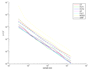
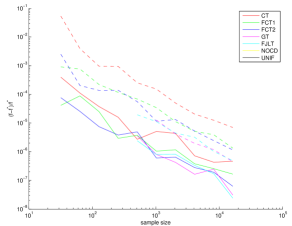
$A_{1}$	$A_{2}$
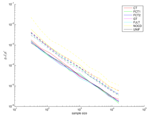
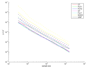
$A_{3}$	$A_{4}$

Figure 5: The first and the third quartiles of relative errors in objective value. The problem size is $2^{18}\times 7$. The first quartiles are drawn in solid lines while the third drawn in dashed lines. If the subsampled problem is rank-deficient, we set corresponding relative error to $\infty$. If a quartile is larger than $100$, we remove it from the plot. There are few differences among those algorithms on $A_{1}$, $A_{3}$, and $A_{4}$. UNIF and NOCD are clearly inferior to algorithms that explore both conditioning and leverage score-based sampling. UNIF and NOCD also failed on $A_{2}$ completely. GT and FJLT failed on $A_{2}$ when the sample size is smaller than $512$. CT works slightly worse than FCT1 and FCT2 on these tests. One interesting fact from the result is that we see $\varepsilon\sim 1/s$ instead of $1/s^{1/2}$.

6.2 Application to $\ell_{1}$ Regression

Next, we embed these transforms into fast approximation of $\ell_{1}$ regression problems to see how they affect the accuracy of approximation. We implement the FastCauchyRegression algorithm of Section 4.2, except that we compute the row norms of $U$ exactly instead of estimating them. Although this takes $O(nd^{2})$ time, it is free from errors introduced by estimating the row norms of $U$, and thus it permits a more direct evaluation of the regression algorithm. Unpublished results indicate that using approximations to the $\ell_{1}$ leverage scores, as is done at the beginning of the FastCauchyRegression algorithm, leads to very similar quality-of-approximation results.

We generate a matrix $A$ of size $2^{18}\times 7$ and generate the right-hand sides $b=Ax_{\text{exact}}+\varepsilon$, where $x_{\text{exact}}$ is a Gaussian vector, and $\varepsilon$ is a random vector whose entries are independently sampled from the Laplace distribution and scaled such that $\|\varepsilon\|_{2}/\|Ax_{\text{exact}}\|_{2}=0.1$. Then, for each row $i$, with probability $0.001$ we replace $b_{i}$ by $100\|\varepsilon\|_{2}$ to simulate corruption in measurements. On this kind of problems, $\ell_{1}$ regression should give very accurate estimate, while $\ell_{2}$ regression won’t work well. For completeness, we also add uniform sampling (UNIF) and no conditioning (NOCD) into the evaluation. Instead of determining the sample size from a given tolerance, we accept the sample size as a direct input; and we choose sample sizes from $2^{5}$ to $2^{14}$.

The results are shown in Figure 5, where we draw the first and the third quartiles of the relative errors in objective value from $50$ independent runs. If the subsampled matrix is rank-deficient, we set corresponding relative error to $\infty$ to indicate a failure. We remove relative errors that are larger than $100$ from the plot in order to show more details. As expected, we can see that UNIF and NOCD are certainly not among reliable choices; they failed (either generating rank-deficient subsampled problems or relative errors larger than $100$) completely on $A_{2}$. In addition, GT and FJLT failed partially on the same test. Empirically, there is not much difference among $\ell_{1}$-based algorithms: CT works slightly worse than FCT1 and FCT2 on these tests, which certainly makes FCT1 and FCT2 more favorable. (One interesting observation is that we find that, in these tests at least, the relative error is proportional to $1/s$ instead of $1/s^{1/2}$. At this time, we don’t have theory to support this observation.) This coupled with the fact that $\ell_{1}$ leverage scores can be approximated more quickly with FCT1 and FCT2 suggests the use of these transforms in larger-scale applications of $\ell_{1}$ regression.

6.3 Evaluation on a Large-scale $\ell_{1}$ Regression Problem

Here, we continue to demonstrate the capability of sampling-based algorithms in large-scale applications by solving a large-scale $\ell_{1}$ regression problem with imbalanced and corrupted measurements. The problem is of size $5.24e9\times 15$, generated in the following way:

1. The true signal $x^{*}$ is a standard Gaussian vector.

2. Each row of the design matrix $A$ is a canonical vector, which means that we only estimate a single entry of $x^{*}$ in each measurement. The number of measurements on the $i$-th entry of $x^{*}$ is twice as large as that on the $(i+1)$-th entry, $i=1,\ldots,14$. We have $2.62$ billion measurements on the first entry while only $0.16$ million measurements on the last. Imbalanced measurements apparently create difficulties for sampling-based algorithms.

3. The response vector is given by

   $$b_{i}=\begin{cases}1000\varepsilon_{i}&\text{with probability }0.001\\ a_{i}^{T}x^{*}+\varepsilon_{i}&\text{otherwise}\end{cases},\quad i=1,\ldots,$$

   where $a_{i}$ is the $i$-th row of $A$ and $\{\varepsilon_{i}\}$ are i.i.d. samples drawn from the Laplace distribution. $0.1\%$ measurements are corrupted to simulate noisy real-world data. Due to these corrupted measurements, $\ell_{2}$ regression won’t give us accurate estimate, and $\ell_{1}$ regression is certainly a more robust alternative.

Since the problem is separable, we know that an optimal solution is simply given by the median of responses corresponding to each entry.

The experiments were performed on a Hadoop cluster with $40$ cores. Similar to our previous test, we implemented and compared Cauchy-conditioned sampling (CT), Gaussian-conditioned sampling (GT), un-conditioned sampling (NOCD), and uniform sampling (UNIF). Since $A$ only has $2n$ non-zeros, CT takes $O(nd\log d)$ time instead of $O(nd^{2}\log d)$, which makes it the fastest among CT, FCT1, and FCT2 on this particular problem. Moreover, even if $A$ is dense, data at this scale are usually stored on secondary storage, and thus time spent on scanning the data typically dominates the overall running time. Therefore, we only implemented CT for this test. Note that the purpose of this test is not to compare CT, FCT1, and FCT2 (which we did above), but to reveal some inherent differences among $\ell_{1}$ conditioned sampling (CT, FCT1, and FCT2), $\ell_{2}$ conditioned sampling (GT and FJLT), and other sampling algorithms (NOCD and UNIF). For each algorithm, we sample approximately $100000$ ($0.019\%$) rows and repeat the sampling $100$ times, resulting $100$ approximate solutions. Note that those $100$ approximate solutions can be computed simultaneously in a single pass.

We first check the overall performance of these sampling algorithms, measured by relative errors in $1$-, $2$-, and $\infty$-norms. The results are shown in Table 4.

	${\|x-x^{*}\|_{1}\over\|x^{*}\|_{1}}$	${\|x-x^{*}\|_{2}\over\|x^{*}\|_{2}}$	${\|x-x^{*}\|_{\infty}\over\|x^{*}\|_{\infty}}$
CT	[0.008, 0.0115]	[0.00895, 0.0146]	[0.0113, 0.0211]
GT	[0.0126, 0.0168]	[0.0152, 0.0232]	[0.0184, 0.0366]
NOCD	[0.0823, 22.1]	[0.126, 70.8]	[0.193, 134]
UNIF	[0.0572, 0.0951]	[0.089, 0.166]	[0.129, 0.254]

Table 4: The first and the third quartiles of relative errors in $1$-, $2$-, and $\infty$-norms. CT clearly performs the best. GT follows closely. NOCD generates large errors, while UNIF works but it is about a magnitude worse than CT.

Since the algorithms are all randomized, we show the first and the third quartiles of the relative errors in $100$ independent runs. We see that CT clearly performs the best, followed by GT. UNIF works but it is about a magnitude worse than CT. NOCD is close to UNIF at the first quartile, but makes very large errors at the third. Without conditioning, NOCD is more likely to sample outliers because the response from a corrupted measurement is much larger than that from a normal measurement. However, those corrupted measurements contain no information about $x^{*}$, which leads to NOCD’s poor performance. UNIF treats all the measurements the same, but the measurements are imbalanced. Although we sample $100000$ measurements, the expected number of measurements on the last entry is only $3.05$, which downgrades UNIF’s overall performance.

We continue to analyze entry-wise errors. Figure 6 draws the first and the third quartiles of entry-wise absolute errors, which clearly reveals the differences among $\ell_{1}$ conditioned sampling, $\ell_{2}$ conditioned sampling, and other sampling algorithms.

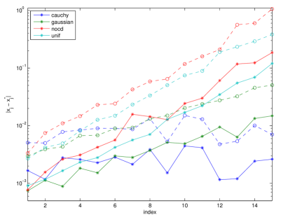
Figure 6: The first (solid) and the third (dashed) quartiles of entry-wise absolute errors for our large-scale $\ell_{1}$ regression empirical evaluation. See the text for details.

While UNIF samples uniformly row-wise, CT tends to sample uniformly entry-wise. Although not as good as other algorithms on the first entry, CT maintains the same error level across all the entries, delivering the best overall performance. The $\ell_{2}$-based GT sits between CT and UNIF. $\ell_{2}$ conditioning can help detect imbalanced measurements to a certain extent and adjust the sampling weights accordingly, but it is still biased towards the measurements on the first several entries.

To summarize, we have shown that $\ell_{1}$ conditioned sampling indeed works on large-scale $\ell_{1}$ regression problems and its performance looks promising. We obtained about two accurate digits ($0.01$ relative error) on a problem of size $5.24e9\times 15$ by passing over the data twice and sampling only $100000$ $(0.019\%)$ rows in a judicious manner.

7 Conclusion

We have introduced the Fast Cauchy Transform, an $\ell_{1}$-based analog of fast Hadamard-based random projections. We have also demonstrated that this fast $\ell_{1}$-based random projection can be used to develop algorithms with improved running times for a range of $\ell_{1}$-based problems; we have provided extensions of these results to $\ell_{p}$; and we have provided the first implementation and empirical evaluation of an $\ell_{1}$-based random projection. Our empirical evaluation clearly demonstrates that for large and very rectangular problems, for which low-precision solutions are acceptable, our implementation follows our theory quite well; and it also points to interesting connections between $\ell_{1}$-based projections and $\ell_{2}$-based projections in practical settings. Understanding these connections theoretically, exploiting other properties such as sparsity, and using these ideas to develop improved algorithms for high-precision solutions to large-scale $\ell_{1}$-based problems, are important future directions raised by our work.

Appendix A Proofs of Technical Cauchy Lemmas

A.1 Proof of Lemma 3 (Cauchy Upper Tail Inequality)

The proof uses similar techniques to the bounds due to Indyk [15] for sums of independent clipped half-Cauchy random variables. Fix $M>0$ (we will choose $M$ later) and define the events

$$F_{i}=\{|C_{i}|\leq M\},$$

and $F=\cap_{i\in[m]}F_{i}$. Note that $F\cap F_{i}=F$. Using the pdf of a Cauchy and because $\tan^{-1}x\leq x$, we have that:

$$\hbox{\bf{Pr}}[F_{i}]={2\over\pi}\tan^{-1}\left(M\right)=1-{2\over\pi}\tan^{-1}\left({1\over M}\right)\geq 1-{2\over\pi M}.$$

By a union bound, $\hbox{\bf{Pr}}[F]\geq 1-{2m\over\pi M}$. Further, $\hbox{\bf{Pr}}[F|F_{i}]\hbox{\bf{Pr}}[F_{i}]=\hbox{\bf{Pr}}[F\cap F_{i}]=\hbox{\bf{Pr}}[F]$, hence $\hbox{\bf{Pr}}[F|F_{i}]=\hbox{\bf{Pr}}[F]/\hbox{\bf{Pr}}[F_{i}]$. We now bound $\hbox{\bf{E}}\left[|C_{i}|\ \bigl{|}\ F\right]$. First, observe that

$$\hbox{\bf{E}}\left[|C_{i}|\ \bigl{|}\ F_{i}\right] = \hbox{\bf{E}}\left[|C_{i}|\ \bigl{|}\ F_{i}\cap F\right]\hbox{\bf{Pr}}[F|F_{i}]+\hbox{\bf{E}}\left[|C_{i}|\ \bigl{|}\ F_{i}\cap\bar{F}\right]\hbox{\bf{Pr}}[\bar{F}|F_{i}]$$

$$\geq \hbox{\bf{E}}\left[|C_{i}|\ \bigl{|}\ F_{i}\cap F\right]\hbox{\bf{Pr}}[F|F_{i}].$$

Next, since $F_{i}\cap F=F$, we have that

$$\hbox{\bf{E}}\left[|C_{i}|\ \bigl{|}F\right]\leq{\hbox{\bf{E}}\left[|C_{i}|\ \bigl{|}\ F_{i}\right]\over\hbox{\bf{Pr}}[F|F_{i}]}={\hbox{\bf{E}}\left[|C_{i}|\ \bigl{|}\ F_{i}\right]\hbox{\bf{Pr}}[F_{i}]\over\hbox{\bf{Pr}}[F]}.$$

Finally, by using the pdf of a Cauchy, $\hbox{\bf{E}}\left[|C_{i}|\bigl{|}F_{i}\right]={{1\over\pi}\log(1+M^{2})}/{\hbox{\bf{Pr}}[F_{i}]}$, and so

$$\hbox{\bf{E}}\left[|C_{i}|\ \bigl{|}F\right]\leq{{1\over\pi}\log(1+M^{2})\over\hbox{\bf{Pr}}[F]}\leq{{1\over\pi}\log(1+M^{2})\over 1-2m/\pi M}.$$

We conclude that

$$\hbox{\bf{E}}[X|F]=\sum_{i\in[m]}\gamma_{i}\hbox{\bf{E}}\left[|C_{i}|\ \bigl{|}F\right]\leq{\gamma\over\pi}\cdot{\log(1+M^{2})\over 1-2m/\pi M}.$$

By Markov’s inequality and because $\hbox{\bf{Pr}}[X\geq\gamma t|\bar{F}]\leq 1$, we have:

$$\hbox{\bf{Pr}}[X\geq\gamma t] = \hbox{\bf{Pr}}[X\geq\gamma t|F]\hbox{\bf{Pr}}[F]+\hbox{\bf{Pr}}[X\geq\gamma t|\bar{F}](1-\hbox{\bf{Pr}}[F])$$

$$\leq {1\over\pi t}\cdot{\log(1+M^{2})\over 1-2m/\pi M}+{2m\over\pi M}.$$

The result follows by setting $M=2mt$.

A.2 Proof of Lemma 4 (Cauchy Lower Tail Inequality)

To bound the lower tail, we will use Lemma 1. By homogeneity, it suffices to prove the result for $\gamma=1$. Let $Z_{i}=\gamma_{i}\min(|C_{i}|,M)$. Clearly $Z_{i}\leq\gamma_{i}|C_{i}|$ and so defining $Z=\sum_{i}Z_{i}$, we have that $Z\leq X$ and $\hbox{\bf{Pr}}[X\leq 1-t]\leq\hbox{\bf{Pr}}[Z\leq 1-t]$. Thus, we have that

$$\hbox{\bf{Pr}}[Z\leq 1-t]=\hbox{\bf{Pr}}[Z\leq\hbox{\bf{E}}[Z]-(\hbox{\bf{E}}[Z]-1+t)]\leq\operatorname{exp}\left({-(\hbox{\bf{E}}[Z]-1+t)^{2}\over 2\sum_{i}\hbox{\bf{E}}[Z_{i}^{2}]}\right),$$

where the last step holds by Lemma 1 for $1-t<\hbox{\bf{E}}[Z]$. Using the distribution of the half-Cauchy, one can verify using standard techniques that by choosing $M\approx 1.6768$, $\hbox{\bf{E}}[Z_{i}]=\gamma_{i}$ and $\hbox{\bf{E}}[Z_{i}^{2}]\leq{3\over 2}\gamma_{i}^{2}$, so $\sum_{i}\hbox{\bf{E}}[Z_{i}]=1$ and $\sum_{i}\hbox{\bf{E}}[Z_{i}^{2}]\leq{3\over 2}\sum_{i}\gamma_{i}^{2}\leq{3\over 2\beta^{2}}$. It follows that $\hbox{\bf{Pr}}[Z\leq 1-t]\leq\operatorname{exp}\left(-t^{2}/{\textstyle{3\over\beta^{2}}}\right),$ and the result follows.

A.3 Proof of Lemma 5 ($\ell_{1}$ Sampling Lemma)

First, observe that ${\|DZx\|}_{1}=\sum_{i\in[n]}D_{ii}|Z_{(i)}x|$, and since $\hbox{\bf{E}}[D_{ii}]=1$, $\hbox{\bf{E}}[{\|DZx\|}_{1}]=\sum_{i\in[n]}|Z_{(i)}x|={\|Zx\|}_{1}$. Next, observe that

$$\sum_{i\in[n]}D_{ii}|Z_{(i)}x|-\sum_{i\in[n]}|Z_{(i)}x|=\sum_{\hat{p}_{i}<1}D_{ii}|Z_{(i)}x|-\sum_{\hat{p}_{i}<1}|Z_{(i)}x|,$$

because when $\hat{p}_{i}=1$, that row must be sampled, and so does not contribute to the deviation. So, we only need to analyze the RHS of the above equation. From now on, we only consider those $i$ with $\hat{p}_{i}<1$, in which case $\hat{p}_{i}=s\cdot t_{i}$, where $t_{i}\geq a{\|Z_{(i)}\|}_{1}/{\|Z\|}_{1}$. Let $Q_{i}$ be the (positive) random variable $D_{ii}|Z_{(i)}x|$; either $Q_{i}=0$ or

$$Q_{i}={|Z_{(i)}x|\over\hat{p}_{i}}\leq{{\|Z_{(i)}\|}_{1}{\|x\|}_{\infty}\over\hat{p}_{i}}={{\|Z_{(i)}\|}_{1}{\|x\|}_{\infty}\over st_{i}}\leq{1\over as}{\|Z\|}_{1}{\|x\|}_{\infty}={\gamma\over s},$$

where we defined $\gamma={1\over a}{\|Z\|}_{1}{\|x\|}_{\infty}$. We can also obtain a bound for $\sum_{\hat{p}_{i}<1}\hbox{\bf{Var}}[Q_{i}]$:

$$\sum_{\hat{p}_{i}<1}\hbox{\bf{Var}}[Q_{i}]=\sum_{\hat{p}_{i}<1}\hbox{\bf{Var}}[Q_{i}]\leq\sum_{\hat{p}_{i}<1}\hbox{\bf{E}}[Q_{i}^{2}]=\sum_{\hat{p}_{i}<1}{|Z_{(i)}x|^{2}\over\hat{p}_{i}}=\sum_{\hat{p}_{i}<1}Q_{i}|Z_{(i)}x|\leq{\gamma\over s}{\|Zx\|}_{1},$$

where, in the last inequality, we used the upper bound for $Q_{i}$ and we further upper bounded by summing over all $i\in[n]$. Let $Q=\sum_{i}Q_{i}$ with $Q_{i}\leq\gamma$; the standard Bernstein bound states that

$$\hbox{\bf{Pr}}\left[\left|Q-\hbox{\bf{E}}[Q]\right|>\varepsilon\right]\leq 2\operatorname{exp}\left({-\varepsilon^{2}\over 2\sum_{i}\hbox{\bf{Var}}[Q_{i}]+{2\over 3}\varepsilon\gamma}\right).$$

Plugging in our bounds for $\sum_{i}\hbox{\bf{Var}}[Q_{i}]$ and $\gamma$, we deduce that

$$\hbox{\bf{Pr}}\Bigl{[}\bigl{|}{\|DZx\|}_{1}-{\|Zx\|}_{1}\bigr{|}>\varepsilon{\|Zx\|}_{1}\Bigr{]}\leq 2\operatorname{exp}\left({-\varepsilon^{2}{\|Zx\|}_{1}^{2}\over{2\gamma\over s}{\|Zx\|}_{1}+{2\varepsilon\gamma\over 3s}{\|Zx\|}_{1}}\right).$$

The lemma follows after some simple algebraic manipulations.

Appendix B Proof of Theorem 1 (Fast Cauchy Transform (FCT1))

Preliminaries.

Before presenting the proof, we describe the main idea. It follows a similar line of reasoning to [24], and it uses an “uncertainty principle” (which we state as Lemma 7 below).

The uncertainty principle we prove follows from the fact that the concatenation of the Hadamard matrix with the identity matrix is a dictionary of low coherence. For background, and similar arguments to those we use in Lemma 7 below, see Section 4 of [16]. In particular, see Claim 4.1 and Lemma 4.2 of that section.

To prove the upper bound, we use the existence of a $(d,1)$-conditioned basis $U$ and apply $\Pi_{1}$ to this basis to show that ${\|\Pi_{1}Ux\|}_{1}$ cannot expand too much, which in turn means that ${\|\Pi_{1}Ax\|}_{1}$ cannot expand too much (for any $x$). To prove the lower bound, we show that the inequality holds with exponentially high probability, for a particular $y$; and we then use a suitable $\gamma$-net to obtain the result for all $y$.

Main Proof.

We now proceed with the proof of Theorem 1. We will first prove an upper bound (Proposition 1) and then a lower bound (Proposition 2); the theorem follows by combining Propositions 1 and 2.

Proposition 1.

With probability at least $1-\delta$, for all $x\in\R^{d}$, $\lVert\Pi_{1}Ax\rVert_{1}\leq\kappa\lVert Ax\rVert_{1}$, where $\kappa=O({d\sqrt{s}\over\delta}\log(r_{1}d))$.

Proof.

Let $U\in\R^{n\times d}$ be a $(d,1)$-conditioned basis (see Definition 2 below) for the column space of $A$, which implies that for some $Z\in\R^{d\times d}$ we can write $A=UZ$. Since $\lVert\Pi_{1}Ax\rVert_{1}\leq\kappa\lVert Ax\rVert_{1}$ if and only if $\lVert\Pi_{1}UZx\rVert_{1}\leq\kappa\lVert UZx\rVert_{1}$, it suffices to prove the proposition for $U$. By construction of $U$, for any $x\in\R^{d}$, $\lVert x\rVert_{\infty}\leq\lVert Ux\rVert_{1}$, and so

$$\lVert\Pi_{1}Ux\rVert_{1}\leq\lVert\Pi_{1}U\rVert_{1}\lVert x\rVert_{\infty}\leq\lVert\Pi_{1}U\rVert_{1}\lVert Ux\rVert_{1}.$$

Thus it is enough to show that $\lVert\Pi_{1}U\rVert_{1}\leq\kappa$. We have

$$\lVert\Pi_{1}U\rVert_{1}=4\lVert BC\tilde{H}U\rVert_{1}=4\sum_{j\in[d]}\lVert BC\tilde{H}U^{(j)}\rVert_{1}=4\sum_{j\in[d]}\lVert BC\hat{U}^{(j)}\rVert_{1},$$

where $\hat{U}\equiv\tilde{H}U$. We will need bounds for $\lVert\hat{U}^{(j)}\rVert_{1}$ for $j\in[d]$, and $\lVert\hat{U}\rVert_{1}$. For any vector $y\in\R^{n}$, we represent $y$ by its $n/s$ blocks of size $s$, so $z_{i}\in\R^{s}$ and $y^{T}=[z_{1}^{T},z_{2}^{T},\ldots,z_{n/s}^{T}]$. Recall that $G_{s}\equiv\left[\begin{smallmatrix}H_{s}\\ I_{s}\end{smallmatrix}\right]$, and observe that $\lVert G_{s}\rVert_{2}=\sqrt{2}$. By explicit calculation,

$$\lVert\tilde{H}y\rVert_{1}=\sum_{i\in[n/s]}\lVert G_{s}z_{i}\rVert_{1}.$$

Since $\lVert G_{s}z_{i}\rVert_{1}\leq\sqrt{2s}\lVert G_{s}z_{i}\rVert_{2}\leq\sqrt{4s}\lVert z_{i}\rVert_{2}\leq\sqrt{4s}\lVert z_{i}\rVert_{1}$, it follows that

$$\lVert\tilde{H}y\rVert_{1}\leq\sqrt{4s}\sum_{i\in[n/s]}\lVert z_{i}\rVert_{1}=\sqrt{4s}\lVert y\rVert_{1}.$$

Applying this to $y=U^{(j)}$ for $j\in[d]$ yields

$$\lVert\hat{U}^{(j)}\rVert_{1}\leq\sqrt{4s}\lVert{U}^{(j)}\rVert_{1},\hbox{ and}\qquad\lVert\hat{U}\rVert_{1}=\sum_{j\in[d]}\lVert\hat{U}^{(j)}\rVert_{1}\leq\sqrt{4s}\lVert U\rVert_{1}\leq d\sqrt{4s},$$ (5)

since $\lVert U\rVert_{1}\leq d$ because $U$ is $(d,1)$-conditioned.

The $(i,j)$ entry of $BC\hat{U}$ is $\sum_{k}B_{ik}C_{kk}{\hat{U}}_{kj},$ which is a Cauchy scaled by $\gamma_{ij}=\sum_{k}|B_{ik}\hat{U}_{kj}|$. So,

$${\|BC\hat{U}\|}_{1}=\sum_{i\in[r_{1}],j\in[d]}\gamma_{ij}\tilde{C}_{ij},$$

where $\tilde{C}_{ij}$ are dependent Cauchy random variables. Using $\sum_{i}B_{ik}=1$, we obtain:

$$\sum_{i,j}\gamma_{ij}=\sum_{i,j,k}|B_{ik}\hat{U}_{kj}|=\sum_{j,k}|\hat{U}_{kj}|\sum_{i}B_{ik}=\sum_{j,k}|\hat{U}_{kj}|={\|\hat{U}\|}_{1}.$$

Hence, we can apply Lemma 3 with $\gamma={\|\hat{U}\|}_{1}$ and $m=r_{1}d$ to obtain

$$\hbox{\bf{Pr}}\left[\lVert BC\hat{U}\rVert_{1}>t\lVert{\hat{U}}\rVert_{1}\right]\leq{(\log(r_{1}d)+\log t)\over t}\left(1+o(1)\right).$$

Setting the RHS to $\delta$, it suffices that $t=O({1\over\delta}\log(dr_{1}))$. Thus, with probability at least $1-\delta$,

$$\lVert BC\hat{U}\rVert_{1}=O\left({1\over\delta}\log(dr_{1})\lVert{\hat{U}}\rVert_{1}\right)=O\left({d\over\delta}\sqrt{s}\log(dr_{1})\right).$$

∎

Before we prove the lower bound, we need the following lemma which is derived using a sparsity result for matrices with unit norm rows and low “coherence,” as measured by the maximum magnitude of the inner product between distinct rows ($G_{s}$ is a matrix with low coherence). This result mimics results in [9, 8, 13, 27, 16].

Lemma 7.

For $G=\left[\begin{smallmatrix}H_{s}\\ I_{s}\end{smallmatrix}\right]$ and any $z\in\R^{s}$, $\lVert Gz\rVert_{1}\geq{1\over 2}s^{1/4}\lVert z\rVert_{2}$.

Proof.

We can assume $\lVert z\rVert_{2}=1$, and so $\lVert Gz\rVert_{2}^{2}=2$. Let $G_{(S^{\prime})}$ be $k$ rows of $G$, with $\kappa$ of them coming from $H_{s}$ and $k-\kappa$ from $I_{s}$. $G_{(S^{\prime})}G_{(S^{\prime})}^{T}=I+\Lambda$ where $\Lambda$ is a symmetric $2\times 2$ block matrix $\left[\begin{smallmatrix}\bm{0}&{1\over\sqrt{s}}Q\\ {1\over\sqrt{s}}Q^{T}&\bm{0}\\ \end{smallmatrix}\right]$ where the entries in $Q\in\R^{\kappa\times(k-\kappa)}$ are $\pm 1$, and so $\lVert Q\rVert_{2}\leq\sqrt{\kappa(k-\kappa)}\leq{1\over 2}k$.

$$\lVert G_{(S^{\prime})}\rVert_{2}^{2}=\lVert G_{(S^{\prime})}G_{(S^{\prime})}^{T}\rVert_{2}\leq 1+\lVert\Lambda\rVert_{2}=1+{1\over\sqrt{s}}\lVert Q\rVert_{2}\leq 1+{k\over 2\sqrt{s}}.$$

Now, given any $z$, we set $k=2\beta\sqrt{s}$ with $\beta={2\over 5}$, and choose $G_{(S^{\prime})}$ to be the rows corresponding to the $k$ components of $Gz$ having largest magnitude, with $G_{(S)}$ being the rows with indices in $[s]\setminus S^{\prime}$. Then $\lVert G_{(S^{\prime})}z\rVert_{2}^{2}\leq 1+\beta$, and so the entry in $G_{(S^{\prime})}z$ with smallest magnitude has magnitude at most $a=\sqrt{(1+\beta)/k}=\sqrt{(1+\beta)/2\beta}s^{-1/4}$. We now consider $G_{(S)}z$. Since $\lVert Gz\rVert_{2}^{2}=2$, $\lVert G_{(S)}z\rVert_{2}^{2}\geq 1-\beta$; further, all components have magnitude at most $a$ (as all the components of $G_{(S)}z$ have smaller magnitude than those of $G_{(S^{\prime})}z$). $\lVert G_{(S)}z\rVert_{1}$ is minimized by concentrating all the entries into as few components as possible. Since the number of non-zero components is at least $(1-\beta)/a^{2}=2\beta s^{1/2}(1-\beta)/(1+\beta)$, giving these entries the maximum possible magnitude results in

$$\lVert G_{(S)}z\rVert_{1}\geq a\times{(1-\beta)\over a^{2}}=(1-\beta)\sqrt{2\beta(1+\beta)}s^{1/4}\geq 0.63s^{1/4}$$

(where we used $\beta={2\over 5}$). We are done because $\lVert Gz\rVert_{1}\geq\lVert G_{(S)}z\rVert_{1}$ ∎

We now prove the lower bound. We assume that Proposition 1 holds for $\Pi_{1}$, which is true with probability at least $1-\delta$ for $\kappa$ as defined in Proposition 1. Then, by a union bound, both Propositions 1 and 2 hold with probability at least

$$1-\delta-\operatorname{exp}\left(-{r_{1}\over 48}+d\log(2d\kappa)\right)-\operatorname{exp}\left(-{s^{1/2}\over 8r_{1}^{2}}+\log r_{1}+d\log(2d\kappa)\right)$$

($\delta$ and $\kappa$ are from Proposition 1). Since $s^{1/2}=r_{1}^{3}$, by choosing $r_{1}=\alpha d\log{d\over\delta}$ for large enough $\alpha$, the final probability of failure is at most $2\delta$, because $\kappa=O({d\sqrt{s}\over\delta}\log(r_{1}d))=O(\operatorname{poly}(d))$.

Proposition 2.

Assume Proposition 1 holds. Then, for all $x\in\R^{d}$, $\lVert\Pi_{1}Ax\rVert_{1}\geq\lVert Ax\rVert_{1}$ holds with probability at least

$$1-\operatorname{exp}\left(-{r_{1}\over 48}+d\log(2d\kappa)\right)-\operatorname{exp}\left(-{s^{1/2}\over 8r_{1}^{2}}+\log r_{1}+d\log(2d\kappa)\right)$$

.

Proof.

First we will show a result for fixed $y\in\R^{n}$, summarized in the next lemma.

Lemma 8.

$\displaystyle\hbox{\bf{Pr}}\left[{\|\Pi_{1}y\|}_{1}<2{\|y\|}_{1}\right]\leq\operatorname{exp}\left(-{{r_{1}\over 48}}\right)+\operatorname{exp}\left(-{s^{1/2}\over 8r_{1}^{2}}+\log r_{1}\right)$

Given this lemma, the proposition follows by putting a $\gamma$-net $\Gamma$ on the range of $A$ (observe that the range of $A$ has dimension at most $d$). This argument follows the same line as in Sections 3 and 4 of [24]. Specifically, let $L$ be any fixed (at most) $d$ dimensional subspace of $\R^{n}$ (in our case, $L$ is the range of $A$). Consider the $\gamma$-net on $L$ with cubes of side $\gamma/d$. There are $(2d/\gamma)^{d}$ such cubes required to cover the hyper-cube ${\|y\|}_{\infty}\leq 1$; and, for any two points $y_{1},y_{2}$ inside the same $\gamma/d$-cube, $\lVert y_{1}-y_{2}\rVert_{1}\leq\gamma$. From each of the $\gamma/d$-cubes, select a fixed representative point which we will generically refer to as $y^{*}$; select the representative to have $\lVert y^{*}\rVert_{1}=1$ if possible. By a union bound and Lemma 8,

$$\hbox{\bf{Pr}}\left[\min_{y^{*}}{\|\Pi_{1}y^{*}\|}_{1}/{\|y^{*}\|}_{1}<2\right]\leq(2d/\gamma)^{d}\left(\operatorname{exp}\left(-{{r_{1}\over 48}}\right)+\operatorname{exp}\left(-{s^{1/2}\over 8r_{1}^{2}}+\log r_{1}\right)\right).$$

We will thus condition on the high probability event that ${\|\Pi_{1}y^{*}\|}_{1}\geq 2{\|y^{*}\|}$ for all $y^{*}$. For any $y\in L$ with ${\|y\|}_{1}=1$, let $y^{*}$ denote the representative point for the cube in which $y$ resides (${\|y^{*}\|}_{1}=1$ as well). Then ${\|y-y^{*}\|}\leq\gamma$.

$${\|\Pi_{1}y\|}_{1}={\|\Pi_{1}y^{*}+\Pi_{1}(y-y^{*})\|}_{1}\geq{\|\Pi_{1}y^{*}\|}_{1}-{\|\Pi_{1}(y-y^{*})\|}_{1}\geq 2{{\|y^{*}\|}_{1}}-\kappa{\|y-y^{*}\|}_{1},$$

where the last inequality holds using Proposition 1. By choosing $\gamma=1/\kappa$ and recalling that ${\|y^{*}\|}_{1}=1$, we have that ${\|\Pi_{1}y\|}_{1}\geq 1$, with probability at least

$$1-\operatorname{exp}(d\log(2d\kappa))\left(\operatorname{exp}\left(-{{r_{1}\over 48}}\right)+\operatorname{exp}\left(-{s^{1/2}\over 8r_{1}^{2}}+\log r_{1}\right)\right).$$

All that remains is to prove Lemma 8. As in the proof of Proposition 1, we represent any vector $y\in\R^{n}$ by its $n/s$ blocks of size $s$, so $z_{i}\in\R^{s}$ and $y^{T}=[z_{1}^{T},z_{2}^{T},\ldots,z_{n/s}^{T}]$. Let $g=\tilde{H}y$,

$$g=\left[\begin{smallmatrix}G_{s}z_{1}\\ G_{s}z_{2}\\ \vdots\\ G_{s}z_{n/s}\end{smallmatrix}\right].$$

We have that ${\|g\|}_{2}^{2}=\sum_{i}{\|G_{s}z_{i}\|}_{2}^{2}=2\sum_{i}{\|z_{i}\|}_{2}^{2}=2{\|y\|}_{2}^{2}$, and

$${\|g\|}_{1}=\sum_{i}{\|G_{s}z_{i}\|}_{1}\geq{1\over 2}s^{1/4}\sum_{i}{\|z_{i}\|}_{2}\geq{1\over 2}s^{1/4}\left(\sum_{i}{\|z_{i}\|}_{2}^{2}\right)^{1/2}={1\over 2}s^{1/4}{\|y\|}_{2}.$$

We conclude that ${\|g\|}_{1}\geq{1\over 2\sqrt{2}}s^{1/4}{\|g\|}_{2}$, which intuitively means that $g$ is “spread out.” We now analyze ${\|BCg\|}_{1}$. (Recall that $\Pi_{1}y=4BCg$, where $g=\tilde{H}y$).

$$(BCg)_{j}=\sum_{i=1}^{2n}B_{ji}C_{ii}g_{i}$$

is a Cauchy random variable $\tilde{C}_{j}$ scaled by $\gamma_{j}=\sum_{i=1}^{2n}B_{ji}|g_{i}|$. Further, because each column of $B$ has exactly one non-zero element, the $\tilde{C}_{j}$ for $j\in[r_{1}]$ are independent. Thus, the random variables ${\|BCg\|}_{1}$ and $\sum_{j\in[r_{1}]}|\tilde{C}_{j}|\gamma_{j}$ have the same distribution. To apply Lemma 4, we need to bound $\sum_{j}\gamma_{j}$ and $\sum_{j}\gamma_{j}^{2}$. First,

$$\sum_{j\in[r_{1}]}\gamma_{j}=\sum_{j\in[r_{1}]}\sum_{i\in[n]}B_{ji}|g_{i}|=\sum_{i\in[n]}|g_{i}|\sum_{j\in[r_{1}]}B_{ji}=\sum_{i=1}^{2n}|g_{i}|={\|g\|}_{1},$$

where the last inequality is because $B^{(i)}$ is a standard basis vector. To bound $\sum_{j}\gamma_{j}^{2}$, we will show that $\gamma_{j}$ is nearly uniform. Since $\gamma_{j}$ is a weighted sum of independent Bernoulli random variables (because $B_{ji}$ and $B_{jk}$ are independent for $i\not=k$), we can use Lemma 2 with $\xi_{i}=|g|_{i}$ and $1-p=1-1/r_{1}\leq 1$, and so $\sum_{i}\xi_{i}={\|g\|}_{1}$ and $\sum_{i}\xi_{i}^{2}={\|g\|}^{2}_{2}$; setting $t=1/r_{1}$ in Lemma 2:

$$\hbox{\bf{Pr}}\left[\gamma_{j}\geq{2{\|g\|}_{1}\over r_{1}}\right]\leq\operatorname{exp}\left(-{{\|g\|}_{1}^{2}\over 2{\|g\|}_{2}^{2}r_{1}^{2}}\right)\leq\operatorname{exp}\left(-{s^{1/2}\over 8r_{1}^{2}}\right).$$

By a union bound, none of the $\gamma_{j}$ exceed $2{\|g\|}_{1}/r_{1}$ with probability at most $r_{1}\operatorname{exp}\left(-{s^{1/2}}/{8r_{1}^{2}}\right)$. We assume this high probability event, in which case $\sum_{j}\gamma_{j}^{2}\leq 4{\|g_{1}\|}^{2}_{1}/r_{1}$. We can now apply Lemma  4 with $\beta^{2}=r_{1}/4$ and $t={1\over 2}$ to obtain

$$\hbox{\bf{Pr}}\left[\sum_{j\in[r_{1}]}|\tilde{C}_{j}|\gamma_{j}\leq{\textstyle{1\over 2}}{\|g\|}_{1}\right]\leq\operatorname{exp}\left(-{{r_{1}\over 48}}\right).$$

By a union bound, ${\|BCg\|}_{1}\geq{1\over 2}{\|g\|}_{1}$ with probability at least $1-\operatorname{exp}\left(-{{r_{1}\over 48}}\right)-\operatorname{exp}\left(-{s^{1/2}\over 8r_{1}^{2}}+\log r_{1}\right)$. Scaling both sides by $4$ gives the lemma. ∎

Running Time.

The running time follows from the time to compute the product $H_{s}x$ for a Hadamard matrix $H_{s}$, which is $O(s\log s)$ time. The time to compute $\tilde{H}y$ is dominated by $n/s$ computations of $H_{s}z_{i}$, which is a total of $O({n\over s}\cdot s\log s)=O(n\log s)$ time. Since $C$ is diagonal, pre-multiplying by $C$ is $O(n)$ and further pre-multiplying by $B$ takes time $O(nnz(B))$, the number of non-zero elements in $B$ (which is $2n$). Thus the total time is $O(n\log s+n)=O(n\log r_{1})$ as desired.

Appendix C Proof of Theorem 2 (Fast Cauchy Transform (FCT2))

Preliminaries.

We will need results from prior work, which we paraphrase in our notation.

Definition 7 (Definition 2.1 of [2]).

For $\varepsilon\in(0,{1\over 2}]$, a distribution on $s\times t$ real matrices $G$ $(s\leq t)$ has the Manhattan Johnson-Lindenstrauss property (MJLP) if for any (fixed) vector $x\in\mathbb{R}^{t}$, the inequalities

$$(1-\varepsilon){\|x\|}_{2}\leq{\|Gx\|}_{2}\leq(1+\varepsilon){\|x\|}_{2}$$

$$c_{3}{\sqrt{s}}(1-\varepsilon){\|x\|}_{2}\leq{\|Gx\|}_{1}\leq c_{3}{\sqrt{s}}(1+\varepsilon){\|x\|}_{2}$$

holds with probability at least $1-c_{1}e^{-c_{2}k\varepsilon^{2}}$ (w.r.t. $G$), for global constants $c_{1},c_{2},c_{3}>0$.

Remark. This is the standard Johnson-Lindenstrauss property with the additional requirement on ${\|Gx\|}_{1}$. Essentially it says that $Gx$ is a nearly uniform, so that ${\|Gx\|}_{1}\approx\sqrt{s}{\|Gx\|}_{2}\approx\sqrt{s}{\|x\|}_{2}$.

Lemma 9 (Theorem 2.2 of [2]).

Let $\eta>0$ be an arbitrarily small constant. For any $s,t$ satisfying $s\leq t^{1/2-\eta}$, there exists an algorithm that constructs a random $s\times t$ matrix $G$ that is sampled from an MJLP distribution with $c_{3}=\sqrt{{2\over\pi}}$. Further, the time to compute $Gx$ for any $x\in\mathbb{R}^{t}$ is $O(t\log s)$.

We will need these lemmas to get a result for how an arbitrary subspace $L$ behaves under the action of $G$, extending Lemma 9 to every $x\in L$, not just a fixed $x$. In the next lemma, the 2-norm bound can be derived using Lemma 9 (above) and Theorem 19 of [18] by placing a $\gamma$-net on $L$ and bounding the size of this $\gamma$-net. (See Lemma 4 of [3].) The Manhattan norm bound is then derived using a second $\gamma$-net argument together with an application of the 2-norm bound. The constants $c_{1},\ c_{2}$ and $c_{3}$ in this lemma are from Definition 7; and the $G$ in Lemmas 9 and 10, with the constants $c_{1},\ c_{2}$ and $c_{3}$ from Definition 7, is the same $G$ used in our FCT2 construction for $\tilde{H}$. We present the complete proof of Lemma 10 in Appendix J.

Lemma 10.

Let $L$ be any (fixed) $d$ dimensional subspace of $\R^{t}$, and $G$ an $s\times t$ matrix sampled from a distribution having the MJLP property. Given $\varepsilon\in(0,{1\over 3}]$, let $s=36(k+{8d\over c_{3}\varepsilon}+\log(2c_{1}))/c_{2}\varepsilon^{2}=O({k\over\varepsilon^{2}}+{d\over\varepsilon^{3}})$. Then, with probability at least $1-e^{-k}$, for every $x\in\R^{t}$,

$$\sqrt{1-\varepsilon}{\|x\|}_{2}\leq{\|Gx\|}_{2}\leq\sqrt{1+\varepsilon}{\|x\|}_{2}$$

$$c_{3}{\sqrt{s}}(1-\varepsilon){\|x\|}_{2}\leq{\|Gx\|}_{1}\leq c_{3}{\sqrt{s}}(1+\varepsilon){\|x\|}_{2}$$

We also need a result on how the matrix of Cauchy random variables $C$ behaves when it hits a vector $y$. The next theorem is Theorem 5 of [24]. For completeness and also to fix some minor errors in the proof of [24], we give a proof of Theorem 12 in Appendix I.

Theorem 12.

Let $L$ be an arbitrary (fixed) subspace of $\mathbb{R}^{n}$ having dimension at most $d$, and $C$ an $r_{1}\times n$ matrix of i.i.d. Cauchy random variables with $r_{1}=c\cdot d\log{d\over\delta}$ for large enough constant $c$. Then, with probability at least $1-\delta$, and for all $y\in L$,

$$\|y\|_{1}\leq{\textstyle{4\over r_{1}}}\|Cy\|_{1}\leq\kappa^{\prime}\|y\|_{1},$$

where $\kappa^{\prime}=O({d\over\delta}\log(r_{1}d))$.

Note that for $\delta$ fixed to some small error probability, $r_{1}=O(d\log d)$, and the product $Cy$ in the theorem above can be computed in time $O(r_{1}n)=O(nd\log d).$

Main Proof.

We now proceed with the proof of Theorem 2. We need to analyze the product $C\tilde{H}Ax$ for all $x\in\R^{d}$. Let $y=Ax\in\R^{n}$, so that $y\in\operatorname{colsp}A\equiv\{Az\mid z\in\R^{d}\}$, and the column space $\operatorname{colsp}A$ is a $d$-dimensional subspace of $\R^{n}$. Partition the coordinate set $[n]$ into $n/t$ contiguous groups of $t$ coordinates. We will work with the block representation of $y$, as defined by this partition, i.e., with $y^{T}=[z_{1}^{T},z_{2}^{T},\ldots,z_{n/t}^{T}]$, where $z_{i}=A_{(\{i\})}x$ and where $A_{(\{i\})}$ is the block of $t$ rows in $A$ corresponding to the indices in $z_{i}$. Then,

$$\tilde{H}y=\left[\begin{smallmatrix}Gz_{1}\\ Gz_{2}\\ \vdots\\ Gz_{n/t}\end{smallmatrix}\right].$$

The vector $z_{i}\in\operatorname{colsp}A_{(\{i\})}$, noting that $\operatorname{colsp}A_{(\{i\})}$ is a subspace of $\R^{t}$ of dimension at most $d$. Let $U_{i}\in\R^{t\times d}$ be an orthonormal basis for $\operatorname{colsp}A_{(\{i\})}$, and let $z_{i}=U_{i}w_{i}$. Setting $\varepsilon={1\over 2}$ in Lemma 10, and recalling that $G$ is $s\times t$, $k$ in Lemma 10 can be expressed as $k={c_{2}s\over 144}-{16d\over c_{3}}-\log(2c_{2})$. Applying a union bound, we have that for all $i\in[n/t]$ with probability at least $1-2c_{1}\cdot{n\over t}\cdot\operatorname{exp}(-{c_{2}s\over 144}+{16d\over c_{3}})$, that for all $y=Ax$ (and corresponding $z_{i}\in\R^{t}$), it holds that

$$\sqrt{\textstyle{1\over 2}}{\|z_{i}\|}_{2}\leq{\|Gz_{i}\|}_{2}\leq\sqrt{\textstyle{3\over 2}}{\|z_{i}\|}_{2}$$

$${\textstyle{1\over 2}}c_{3}\sqrt{s}{\|z_{i}\|}_{2}\leq{\|Gz_{i}\|}_{1}\leq{\textstyle{3\over 2}}c_{3}\sqrt{s}{\|z_{i}\|}_{2}$$ .

We will condition on this event, which occurs with high probability for the given parameters. We can now bound ${\|\tilde{H}y\|}_{1}=\sum_{i\in[n/t]}\|Gz_{i}\|_{1}$ as follows.

$${\|\tilde{H}y\|}_{1} = \sum_{i\in[n/t]}\|Gz_{i}\|_{1}\leq{\textstyle{3\over 2}}c_{3}\sqrt{s}\sum_{i\in[n/t]}\|z_{i}\|_{2}\leq{\textstyle{3\over 2}}c_{3}\sqrt{s}\sum_{i\in[n/t]}\|z_{i}\|_{1}={\textstyle{3\over 2}}c_{3}\sqrt{s}{\|y\|}_{1};$$ (6)

$${\|\tilde{H}y\|}_{1} = \sum_{i\in[n/t]}\|Gz_{i}\|_{1}\geq{\textstyle{1\over 2}}c_{3}\sqrt{s}\sum_{i\in[n/t]}\|z_{i}\|_{2}\geq{\textstyle{1\over 2}}c_{3}\sqrt{\textstyle{s\over t}}\sum_{i\in[n/t]}\|z_{i}\|_{1}={\textstyle{1\over 2}}c_{3}\sqrt{\textstyle{s\over t}}{\|y\|}_{1};$$ (7)

Since $\operatorname{colsp}\tilde{H}A$ has dimension at most $d$, we can apply Theorem 12 to it. We have that with probability at least $1-\delta$, for all $x\in\mathbb{R}^{d}$,

$$\|\tilde{H}Ax\|_{1}\leq{4\over r_{1}}\|C\tilde{H}Ax\|_{1}\leq\kappa^{\prime}\|\tilde{H}Ax\|_{1},$$

where $\kappa^{\prime}=O({d\over\delta}\log(r_{1}d))$ from Theorem 12. Recall that $\Pi_{1}\equiv{8\over r_{1}}\sqrt{{\pi t\over 2s}}C\tilde{H}$. We now use (6) and (7) with $y=Ax$, and after multiplying by ${2\over c_{3}}\sqrt{{t\over s}}$ and setting $c_{3}=\sqrt{2/\pi}$, we conclude that for all $x\in\mathbb{R}^{d}$,

$$\|Ax\|_{1}\leq\|\Pi_{1}Ax\|_{1}\leq 3\kappa^{\prime}\sqrt{t}\|Ax\|_{1}$$ (8)

holds with probability at least $1-\delta-2c_{1}\cdot{n\over t}\operatorname{exp}(-{c_{2}s\over 144}+{16d\over c_{3}})\geq 1-2\delta$ (by choosing $s\geq{144\over c_{2}}({16d\over c_{3}}+\log{2c_{1}n\over\delta t})$). The theorem follows because $\log n\leq d$ and hence $\kappa^{\prime}=O({d\over\delta}\log d)$, $s=O(d+\log{1\over\delta})$ and $t=O(s^{2+\eta})$.

Running Time.

We now evaluate the time to compute $\Pi_{1}y$ for $y\in\R^{n}$. We first compute $\tilde{H}y$ which requires $n/t$ computations of $Gz_{i}$. Since $s=t^{1/2-\eta/2}$, we can invoke Lemma 9. The time to compute all $Gz_{i}$ is ${n\over t}\cdot t\log s=n\log s$. Since $\tilde{H}y$ is $(ns/t)\times 1$, it takes $O(r_{1}ns/t)$ time to compute $C\tilde{H}y$, which concludes the computation. The total running time is $O(n\log s+nr_{1}s/t)$. Using $\log n\leq d$, $s=O(d)$, $t=s^{2+\eta}$, $r_{1}=O(d\log{d\over\delta})$ we need total time $O(n\log{d\over\delta})$. To compute $\Pi_{1}A$, we need to compute $\Pi_{1}A^{(j)}$ for $d$ vectors $A^{(j)}$, resulting in a total run time $O(nd\log{d\over\delta})$.

Appendix D Proof of Theorem 3 (Fast $\ell_{1}$ Well-conditioned Basis)

Clearly $U=AR^{-1}$ is in the range of $A$ and has the same null-space otherwise $\Pi_{1}A$ would not preserve lengths to relative error. Therefore $U$ is a basis for the range of $A$. Consider any $x\in\R^{d}$. The first claim of the theorem follows from the following derivations:

$${\|U\|}_{1}={\|AR^{-1}\|}_{1}\mathop{\buildrel(a)\over{\leq}}{\|\Pi_{1}AR^{-1}\|}_{1}\mathop{\leq}\sqrt{r_{1}}{\|\Pi_{1}AR^{-1}\|}_{2}{\buildrel(b)\over{=}}d\sqrt{r_{1}};\mbox{and}$$

$${\|x\|}_{\infty}\mathop{\leq}{\|x\|}_{2}\mathop{\buildrel(b)\over{=}}{\|\Pi_{1}AR^{-1}x\|}_{2}\leq{\|\Pi_{1}AR^{-1}x\|}_{1}{\buildrel(c)\over{\leq}}\kappa{\|AR^{-1}x\|}_{1}=\kappa{\|Ux\|}_{1}.$$

(a) follows from the lower bound in (3), because it holds for every column of $AR^{-1}$; (b) follows because by the construction of $R$, $\Pi_{1}AR^{-1}$ has $d$ orthonormal columns; finally, (c) follows from the upper bound in (3).

Finally, to obtain the Corollary, if $\Pi_{1}$ satisfying (3) is constructed using Theorem 2 with small fixed probability of failure $\delta$, then $r_{1}=O(d\log d)$ and $\kappa=O(d^{2+\eta}\log d)$. The running time to compute ${R^{-1}}$ is obtained by summing $O(nd\log d)$ (to compute $\Pi_{1}A$) and $O(r_{1}d^{2})=O(d^{3}\log d)$ (to obtain $R^{-1}\in\R^{d\times d}$).

Appendix E Proof of Theorem 4 (Fast Cauchy $\ell_{1}$ Regression)

For $X\in\R^{n\times q}$, we analyze the more general constrained $\ell_{1}$ regression problem, $\min_{x\in{\cal C}}{\|Xx\|}_{1},$ where ${\cal C}\subseteq\R^{q}$ is a convex set, and we show that $\hat{x}\in{\cal C}$ constructed by our algorithm is a $(1+\varepsilon)$-approximation for this more general problem:

$${\|X\hat{x}\|}_{1}\leq(1+\varepsilon)\min_{x\in{\cal C}}{\|Xx^{*}\|}_{1}.$$

(That is, we actually prove a somewhat stronger result than we state in Theorem 4. This more general problem involves calling our main algorithm with $b=\{\}$ (NULL), and then incorporating the constraint that $x\in{\cal C}$ into the optimization problem that is solved as a black box in the last step. Of course, if the constraint set is not a polytope, then the last step may involve more sophisticated techniques than linear programming.) The classic $\ell_{1}$ regression is obtained by setting $X=\left[\begin{matrix}A&-b\end{matrix}\right]$ ($q=d+1$) with constraint ${\cal C}=\{x:e_{d+1}^{T}x=1\}$, which corresponds to setting $x_{d+1}=1$.

The main ingredients in our proof follow a similar line to those in [6, 7, 24]. We use the notation from Figure 2. From Step 1, $\Pi_{1}$ satisfies (3) with $A\leftarrow X$, i.e., $\Pi_{1}$ preserves the $\ell_{1}$-norm of vectors in the range of $X$:

$${\|Xx\|}_{1}\leq{\|\Pi_{1}Xx\|}_{1}\leq\kappa{\|Xx\|}_{1}.$$ (9)

Let ${\cal C}^{\prime}=\{y={R^{-1}}x:x\in{\cal C}\}$ be a linear transform of the constraint set. We start with a basic lemma that allow us to use $U$ instead of $X$. This lemma says that if we can construct a sampling matrix $D$ for $U$ under the constraint ${\cal C}^{\prime}$ such that solving the down-sampled problem for $U$ gives a $(1+\varepsilon)$-approximation, then that same sampling matrix works for $X$ under the constraint ${\cal C}$.

Lemma 11.

Let $U=X{R^{-1}}$ and $D$ any diagonal sampling matrix as in Figure 2. Suppose that for any $\hat{y}\in{\cal C}^{\prime}$ that minimizes ${\|DUy\|}$, $\hat{y}$ is a $(1+\varepsilon)$-approximation for the problem $\min_{y\in{\cal C}^{\prime}}{\|Uy\|}$. Let $\hat{x}$ be any solution to $\min_{x\in{\cal C}}{\|DXx\|}$. Then $\hat{x}$ is a $(1+\varepsilon)$-approximation for the problem $\min_{x\in{\cal C}}{\|Xx\|}$.

Proof.

Select $\hat{y}={R^{-1}}\hat{x}\in{\cal C}^{\prime}$. For any $y\in{\cal C}^{\prime}$, there is some $x\in{\cal C}$ with $y={R^{-1}}x$, and we have:

$${\|DUy\|}_{1}={\|DU{R^{-1}}x\|}_{1}={\|DXx\|}_{1}{\buildrel(a)\over{\geq}}{\|DX\hat{x}\|}_{1}={\|DU{R^{-1}}\hat{x}\|}_{1}={\|DU\hat{y}\|}_{1},$$

where (a) is by the optimality of $\hat{x}$. So, $\hat{y}$ minimizes ${\|DUy\|}_{1}$, hence for all $y\in{\cal C}^{\prime}$, ${\|U\hat{y}\|}_{1}\leq(1+\varepsilon){\|Uy\|}_{1}$. Now consider any $x\in{\cal C}$ and let $y={R^{-1}}x\in{\cal C}^{\prime}$. Then,

$${\|X\hat{x}\|}_{1}={\|U{R^{-1}}\hat{x}\|}_{1}={\|U\hat{y}\|}_{1}\leq(1+\varepsilon){\|Uy\|}_{1}=(1+\varepsilon){\|U{R^{-1}}x\|}_{1}=(1+\varepsilon){\|Xx\|}_{1}.$$

∎

Remarks. We emphasize that our proof accommodates an arbitrary constraint set ${\cal C}$. For the classical $\ell_{1}$ regression problem, that is of interest to us in Theorem 4, we only need ${\cal C}$ to be specified by a single linear constraint. In the remaining, we will work with $U$ and show that our algorithm generates a coreset that works, regardless of the constraint set ${\cal C}^{\prime}$.

By Theorem 3, $U=X{R^{-1}}$ is an $(\alpha,\beta)$-conditioned basis for the range of $X$, where

$$\alpha\leq q\sqrt{r_{1}},\qquad\text{ and }\beta\leq\kappa.$$

So, ${\|U\|}_{1}\leq q\sqrt{r_{1}}$ and for all $y\in\R^{q}$, ${\|y\|}_{\infty}\leq\kappa{\|Uy\|}_{1}$. We next show that $\lambda_{i}$ estimates ${\|U_{(i)}\|}_{1}$. The following lemma is a straightforward application of a Chernoff bound to independent half-Cauchys (see also Claims 1 and 2 and Lemmas 1 and 2 in [15]).

Lemma 12.

Let $Z_{1},\ldots,Z_{r_{2}}$ be $r_{2}$ independent Cauchys. Then, ${1\over 2}\leq\operatorname{median}\{|Z_{1}|,\ldots,|Z_{r_{2}}|\}\leq{3\over 2}$ with probability at least $1-2e^{-cr_{2}}$, where $c\geq 2(\tan^{-1}({1\over 5}))^{2}\geq 0.07$ is a constant.

Fix $i$ and for $j\in[r_{2}]$ define the random variables $Z_{j}=\Lambda_{ij}$ to apply Lemma 12. Observe that for $j\in[r_{2}]$, $Z_{j}=\Lambda_{ij}=U_{(i)}\Pi_{2}^{(j)}$ are independent Cauchy random variables scaled by ${\|U_{(i)}\|}_{1}$. Applying Lemma 12 with $\lambda_{i}=\operatorname{median}_{j\in r_{2}}|\Lambda_{ij}|$, we have that with probability at least $1-2e^{-cr_{2}}$

$${\textstyle{1\over 2}}{\|U_{(i)}\|}_{1}\leq\lambda_{i}\leq{\textstyle{3\over 2}}{\|U_{(i)}\|}_{1}.$$ (10)

By a union bound, these inequalities hold for all $i\in[n]$ with probability at least $1-2ne^{-cr_{2}}\geq 1-\delta$ for $r_{2}\geq{1\over c}\log{2n\over\delta}$ (since ${1\over c}\leq 15$, our algorithm satisfies this condition). Next we show that if the sampling matrix preserves the $\ell_{1}$-norm of every vector in the range of $U$, then we are done.

Lemma 13.

Given $D$ with $n$ columns, Suppose that for all $y\in\R^{q}$,

$$(1-\varepsilon){\|Uy\|}_{1}\leq{\|DUy\|}_{1}\leq(1+\varepsilon){\|Uy\|}_{1},$$ (11)

and suppose that $\hat{y}$ is a solution to $\min_{y\in{\cal C}^{\prime}}{\|DUy\|}$. Then, for all $y\in{\cal C}^{\prime}$,

$${\|U\hat{y}\|}_{1}\leq\left({1+\varepsilon\over 1-\varepsilon}\right){\|Uy\|}_{1}.$$

Proof.

Since $D$ preserves norms, for any $y\in{\cal C}^{\prime}$ we have that:

$${\|U\hat{y}\|}_{1}\leq{1\over 1-\varepsilon}{\|DU\hat{y}\|}_{1}{\buildrel(a)\over{\leq}}{1\over 1-\varepsilon}{\|DUy\|}_{1}\leq{1+\varepsilon\over 1-\varepsilon}{\|Uy\|}_{1}.$$

(a) is by the optimality of $\hat{y}$. ∎

The remainder of the proof is to show that $D$ from our algorithm in Figure 2 satisfies the pre-condition of Lemma 13, namely (11). We need two ingredients. The first is the $\ell_{1}$-sampling lemma Lemma 5. The second ingredient is a standard $\gamma$-net argument.

We are going to apply Lemma 5 with $Z=U$. From (10) (which holds for all $i\in[n]$ with probability at least $1-\delta$), $\lambda_{i}/\sum_{i\in[n]}\lambda_{i}\geq{1\over 3}{\|U_{(i)}\|}_{1}/{\|U\|}_{1}$, and so we can apply Lemma 5 with $a={1\over 3}$. Since $U$ is $(\alpha,\beta)$-conditioned, ${\|Uy\|}_{1}\geq{1\over\beta}{\|y\|}_{\infty}$, and ${\|U\|}_{1}\leq\alpha$, and so we have that with probability at least $1-\delta$,

$$(1-\varepsilon){\|Uy\|}_{1}\leq{\|DUy\|}_{1}\leq(1+\varepsilon){\|Uy\|}_{1},$$

where $\delta\leq 2\operatorname{exp}\left({-s\varepsilon^{2}\over(6+2\varepsilon)\alpha\beta}\right)$, and $\alpha\beta\leq\kappa q\sqrt{r_{1}}$. If $y=\bm{0}$ then the bounds trivially hold; by rescaling, it thus suffices to show the bound for all $y\in\R^{q}$ with ${\|y\|}_{\infty}=1$. We now show this using a standard $\gamma$-net argument. Consider the uniform lattice on $\R^{q}$ specified by $T={\gamma\over q}\mathbb{Z}^{q}$ (we assume that $q/\gamma$ is a positive integer for simplicity). Let $H=\{z:{\|z\|}_{\infty}\leq 1\}\cap T$ be the restriction of this grid to only its points within the hypercube of points with $\ell_{\infty}$-norm equal to 1; $|H|\leq({2q\over\gamma})^{q}$. Consider any $y$ with ${\|y\|}_{\infty}=1$, and let $h$ be the closest grid point in $H$ to $y$. Then

$$y=h+{\gamma\over q}\sum_{i=1}^{q}\zeta_{i}e_{i},$$ (12)

where $0\leq|\zeta_{i}|\leq 1$. Observe that $e_{i}\in H$. By a union bound, for every $h\in H$, with probability at least $1-\delta$,

$$(1-\varepsilon){\|Uh\|}_{1}\leq{\|DUh\|}_{1}\leq(1+\varepsilon){\|Uh\|}_{1},$$

where $\delta\leq 2|H|\operatorname{exp}\left({-s\varepsilon^{2}\over(6+2\varepsilon)\alpha\beta}\right)$. We condition on this high probability event. Then,

$${\|DUy\|}_{1}={\left\|DUh+{\gamma\over q}\sum_{i=1}^{q}\zeta_{i}DUe_{i}\right\|}_{1} \leq {\|DUh\|}_{1}+{\gamma\over q}\sum_{i=1}^{q}|\zeta_{i}|{\|DUe_{i}\|}_{1}$$

$$\leq (1+\varepsilon)\left({\|Uh\|}_{1}+{\gamma\over q}\sum_{i=1}^{q}{\|Ue_{i}\|}_{1}\right).$$

Applying $U$ to both sides of (12) and using the triangle inequality, ${\|Uh\|}_{1}\leq{\|Uy\|}_{1}+{\gamma\over q}\sum_{i=1}^{q}|\zeta_{i}|{\|Ue_{i}\|}_{1}$. We conclude that

$${\|DUy\|}_{1}\leq(1+\varepsilon)\left({\|Uy\|}_{1}+{2\gamma\over q}\sum_{i=1}^{q}{\|Ue_{i}\|}_{1}\right)\leq(1+\varepsilon){\|Uy\|}_{1}\left(1+{2\gamma\alpha\beta\over q}\right),$$

where we used ${\|Uy\|}_{1}\geq{1\over\beta}{\|y\|}_{\infty}={1\over\beta}$ (since ${\|y\|}_{\infty}=1$) and $\sum_{i=1}^{q}{\|Ue_{i}\|}_{1}={\|U\|}_{1}\leq\alpha$. In an analogous way, we get the lower bound:

$${\|DUy\|}_{1}={\left\|DUh+{\gamma\over q}\sum_{i=1}^{q}\zeta_{i}DUe_{i}\right\|}_{1} \geq {\|DUh\|}_{1}-{\gamma\over q}\sum_{i=1}^{q}|\zeta_{i}|{\|DUe_{i}\|}_{1}$$

$$\geq (1-\varepsilon){\|Uh\|}_{1}-{\gamma(1+\epsilon)\over q}\sum_{i=1}^{q}{\|Ue_{i}\|}_{1}$$

$$= (1-\varepsilon){\|Uh\|}_{1}-{\gamma(1+\epsilon)\over q}{\|U\|}_{1}.$$

Again, applying $U$ to (12) and using the triangle inequality gives ${\|Uh\|}_{1}\geq{\|Uy\|}_{1}-{\gamma\over q}{\|U\|}_{1}$. Further, ${\|Uy\|}_{1}\leq{\|U\|}_{1}{\|y\|}_{\infty}\leq\alpha$, and so we have

$${\|DUy\|}_{1}\geq(1-\varepsilon)\left({\|Uy\|}_{1}-{2\gamma\over q(1-\epsilon)}{\|U\|}_{1}\right)\geq(1-\varepsilon){\|Uy\|}_{1}\left(1-{4\gamma\alpha\beta\over q}\right),$$

where we assume $\epsilon\leq{1\over 2}$. Setting $\gamma=q\varepsilon/(4\alpha\beta)$, using $(1+\varepsilon)^{2}\leq 1+3\varepsilon$ and $(1-\varepsilon)^{2}\geq 1-3\varepsilon$ (for $\varepsilon<{1\over 2}$), and rescaling $\varepsilon$ by dividing by 3, we obtain that with probability at least $1-\delta$,

$$(1-\varepsilon){\|Uy\|}_{1}\leq{\|DUy\|}_{1}\leq(1+\varepsilon){\|Uy\|}_{1}.$$

where $\delta\leq 2|H|\operatorname{exp}\left({-s\varepsilon^{2}\over 9(6+2\varepsilon/3)\alpha\beta}\right)$, and $|H|\leq({24\alpha\beta\over\varepsilon})^{q}$. Solving for $s$ using $\alpha\leq q\sqrt{r_{1}}$ and $\beta\leq\kappa$, and simplifying a little, we require

$$s\geq{63\kappa q\sqrt{r_{1}}\over\varepsilon^{2}}\left(q\log{24\kappa q\sqrt{r_{1}}\over\varepsilon}+\log{2\over\delta}\right).$$

The total success probability is $1-2\delta$, which results from a union bound applied to the two random processes involving $\Pi_{2}$ and $D$. The Theorem now follows by setting $\delta=1/d^{\rho}$ for a constant $\rho$. This concludes the proof of the correctness.

Running Time.

Set $\delta={1\over 3q^{\rho}}$, for $\rho=O(1)$. We compute the running time as follows. In Step 2, if we use Theorem 2 for $\Pi_{1}$ (which succeeds with probability $1-\delta$), the time to compute $\Pi_{1}X$ is $O(nq\log q)$ and $r_{1}=O(q\log q)$ and $\kappa=O\left(q^{\rho+2}\log q)\right)$ ($r_{1}$ and $\kappa$ affect the running time of later steps); We need to compute an orthogonal factorization in $O(r_{1}q^{2})$ and then compute ${R^{-1}}$ in $O(q^{3})$ for a total run time of Step 2 that is $O((n+q^{2})q\log q)$. In Step 3, $r_{2}=O(\log n)$ by our choice of $r_{2}$, so the time to compute $\Lambda=X{R^{-1}}\Pi_{2}$ is in $O(nqr_{2}+r_{2}q^{2})=O(nq\log n+q^{2}\log n)$, where $O(nq\log n+q^{2}\log n)$ is the time needed to compute $R^{-1}\Pi_{2}$ followed by $X\cdot(R^{-1}\Pi_{2})$. Note that $q^{2}\log n\leq nq\log n$.

Since computation of the median of $r_{2}$ elements is in $O(r_{2})$, computing all $\lambda_{i}$ takes $O(nr_{2})=O(n\log n)$ time. Thus, the running time for Steps 1-5 is $O(nq\log n)+q^{3}\log q$.

In Step 6, $s=O\left(\varepsilon^{-2}q^{\rho+{9\over 2}}\log^{{5\over 2}}({q\over\varepsilon})\right)$. It takes $O(n)$ time to sample the diagonal matrix $D$ and then $O(qS)$ time to construct $DA$ and $Db$, where $S$ is the number of non-zero entries in $D$. Lastly Step 8 takes $\phi(S,d)=\Omega(dS)$ time to solve the $\ell_{1}$ regression on the smaller problem with $s$ rows in $d$ dimensions. The total running time is thus:

$$O\left(nq\log n+\phi(S,q)\right).$$

where $\hbox{\bf{E}}[S]\leq s=O\left(\varepsilon^{-2}q^{\rho+{9\over 2}}\log^{{5\over 2}}({q\over\varepsilon})\right)$ and $S$ is very tightly concentrated around $s$ (via a standard Bernstein bound) because it is the sum of independent binomial variables; specifically, with probability at least $1-e^{-{3\over 8}s}$, $S\leq 2s$. Hence $S=O(s)$ with probability $1-o(1)$. The probability of success is $1-3\delta=1-{1\over q^{\rho}}$ (union bound). Since $s=\varepsilon^{-2}q^{\rho+{9\over 2}}\operatorname{poly}(\log{q\over\varepsilon})$, and since standard algorithms for linear programming give $\phi(S,q)=Sq^{O(1)}$, we have the result claimed in the theorem for $q=O(d)$.

Appendix F Proof of Theorem 5 (Optimized Fast Cauchy $\ell_{1}$ Regression)

As in the proof of Theorem 4 in Section  E, given is $X\in\R^{n\times q}$ and the constraint set ${\cal C}$. We condition on $\Pi_{1}\in\R^{r_{1}\times n}$ satisfying (3) and Theorem 3. So, $U=XR^{-1}$ is $(q\sqrt{r_{1}},\kappa)$-conditioned where $r_{1}$ and $\kappa$ depend on $n,q,\delta$ (this holds with probability at least $1-\delta$). Thus, ${\|U\|}_{1}\leq q\sqrt{r_{1}}$ and ${\|x\|}_{\infty}\leq\kappa{\|Ux\|}_{1}$ for any $x\in\R^{q}$. It follows that

$${q\over\kappa}\leq{\|U\|}_{1}\leq q\sqrt{r_{1}}.$$

(The lower bound follows from $\sum_{i\in[q]}{\|e_{i}\|}_{\infty}\leq\sum_{i\in[q]}{\|Ue_{i}\|}_{1}$, where $e_{i}$ are standard basis vectors.) In the proof of Theorem 4, we proved the following result. Given weights $t_{i}$, with

$$t_{i}\geq a\cdot{{\|U_{(i)}\|}_{1}\over{\|U\|}_{1}}\qquad\forall i\in[n],$$ (13)

define leverage probabilities

$$\ell_{i}=\min\left(1,s\cdot t_{i}\right),$$

with

$$s\geq{63\kappa q\sqrt{r_{1}}\over a\varepsilon^{2}}\cdot\left(q\log{4q\sqrt{r_{1}}\max(q\sqrt{r_{1}},\kappa)\over\varepsilon}+\log{2\over\delta}\right).$$ (14)

and construct the random diagonal sampling matrix $D$ with $D_{ii}=1/\ell_{i}$ with probability $\ell_{i}$ and zero otherwise. Then, with probability at least $1-\delta$, solving the coreset problem given by $DX$ and the constraints ${\cal C}$ gives a $(1+\varepsilon)/(1-\varepsilon)$ approximate solution to the full $L_{1}$ regression with $X$ and ${\cal C}$. In the proof of Theorem 4, the purpose of $\Pi_{2}$ was to allow us to construct weights $t_{i}$ quickly such that with high probability, ${1\over a}\leq 3$. Here, we show that our faster way to get weights, results in only a $\operatorname{poly}(d\epsilon^{-1}\log n)$ factor increase in ${1\over a}$.

Recall $\Lambda=U\Pi_{2}$, where $\Pi_{2}\in\R^{n\times r_{2}}$ is a matrix of $i.i.d.$ standard Gaussian random variables, and $\hat{\lambda}_{i}=\operatorname{median}_{j\in[r_{2}]}|\Lambda_{ij}|$, with and

$$\hat{p}_{i}=\min\left(1,s\cdot\hat{\lambda}_{i}\right).$$

For $j\in[r_{2}]$, the $\Lambda_{ij}$ are i.i.d. zero mean Gaussians with variance ${\|U_{(i)}\|}_{2}^{2}$, so $|\Lambda_{ij}|$ are i.i.d half Gaussians. We need a result from [15].

Lemma 14.

(Lemma 2 of [15]). Let $x_{1},\ldots,x_{r}$ be i.i.d. with continuous distribution function $F$ and $\lambda=\operatorname{median}_{i\in[r]}x_{i}$. Then,

$$\hbox{\bf{Pr}}\left[\lambda\geq F^{-1}({\textstyle{1\over 2}}-\epsilon)\right]\geq{1-\operatorname{exp}({-2\epsilon^{2}r})},$$

$$\hbox{\bf{Pr}}\left[\lambda\leq F^{-1}({\textstyle{1\over 2}}+\epsilon)\right]\geq{1-\operatorname{exp}({-2\epsilon^{2}r})},$$

For the half Gaussian with variance $\sigma^{2}$, $F(x)=2\phi(x/\sigma)-1$ where $\phi$ is the standard Gaussian distribution function. Choosing $\epsilon={1\over 4}$ and using Lemma 14, with probability at least $1-\operatorname{exp}({-r_{2}/2})$,

$$\hat{\lambda}_{i}\geq 0.3\cdot{\|U_{(i)}\|}_{2}$$

where we used $0.3<\phi^{-1}({\textstyle{5\over 8}})$. Using ${\|U_{(i)}\|}_{2}\geq{\|U_{(i)}\|}_{1}/\sqrt{q}$ and ${\|U\|}_{1}\geq q/\kappa$, it follows that

$$\hat{\lambda}_{i}\geq{0.3\over\sqrt{q}}{\|U_{(i)}\|}_{1}\geq{0.3\sqrt{q}\over\kappa}{{\|U_{(i)}\|}_{1}\over{\|U\|}_{1}}$$ (15)

holds with probability at least $1-2\operatorname{exp}({-r_{2}/2})$ for any particular $i$. If we required these bounds to hold for all $i\in[n]$, then to apply the union bound succesfully, we would need to set $r_{2}=\Omega(\log n)$, which is too costly. We want $r_{2}=O(\log(d\epsilon^{-1}\log n))$, so we need a more subtle argument. We choose $s$ as in (14) with $a=0.3\sqrt{q}/\kappa$.

Let $t_{i}={\|U_{(i)}\|}_{1}$ and $p_{i}=\min(1,s\cdot t_{i})$ be sampling probabilities obtained from the the exact $L_{1}$ leverage scores for $U$. For these sampling probabilities, $a$ in (13) is larger which would imply that a smaller $s$ is needed. Nevertheless, any larger value of $s$ will also work, and so the same value of $s$ with $a=0.3\sqrt{q}/\kappa$ will work with the weights $t_{i}$. Note that since $\Pi_{1}$ is fixed, $p_{i}$ is not a random variable, but $\hat{p}_{i}$ is a random variable depending on $\Pi_{2}$. Fix $r_{2}$ and generate $\Pi_{2}$ and thence $\hat{\lambda}_{i},\hat{p}_{i}$.

We define a set of indices $T\subseteq[n]$ as those $i$ for which $\hat{\lambda}_{i}\geq(0.3\sqrt{q}/\kappa){\|U_{(i)}\|}_{1}/{\|U\|}_{1}$. These are the indices for which $\Pi_{2}$ ‘worked’. Essentially, these are the large leverage scores. The intuition behind our argument is that even though there may be some indices for which $\Pi_{2}$ did not work, there are enough large leverage scores for which $\Pi_{2}$ did work that the probability of these faulty indices coming into play is miniscule.

To make this argument, we define hybrid weights $w_{i}$ to equal $\hat{\lambda}_{i}$ for $i\in T$ and $t_{i}$ for $i\not\in T$. By construction,

$$w_{i}\geq{0.3\sqrt{q}\over\kappa}{{\|U_{(i)}\|}_{1}\over{\|U\|}_{1}},$$

and so the same $s$ works for constructing sampling probabilities $q_{i}=\min(1,s\cdot w_{i})$. Note that in the algorithm, we do not actually construct (or know) $p_{i},q_{i}$; they are just used here as a hypothetical set of sampling probabilities which help us to analyze the performance of the actual sampling probabilities we use, which are $\hat{p}_{i}$. The important property about the $q_{i}$ is that for $i\in T$, $q_{i}=\hat{p}_{i}$.

We call a set of rows that are sampled and rescaled according to a set of probabilities a good coreset if the coreset solution from this sample is a $(1+\varepsilon)$-approximation to the full $L_{1}$ regression. The sampling probabilities $q_{i}$ give a good coreset with probability at least $1-\delta$. We now define several events over three random processes: $\Pi_{2}$, sampling a coreset according to $\hat{p}_{i}$ and sampling a coreset according to $q_{i}$. The last two random processes depend on the outcome of $\Pi_{2}$.

• AllBounded is the event $\{\hat{\lambda}_{i}\leq C\sqrt{\log n}\cdot{\|U_{(i)}\|}_{2}\ \forall i\in[n]\}$ (we will choose $C$ later). We show

  $$\Pr_{\Pi_{2}}[{\sf AllBounded}]\geq 1-{1\over n^{{1\over 2}C^{2}-1}}.$$

  Indeed, $\hat{\lambda}_{i}$ is the median of $r_{2}$ i.i.d. zero mean Gaussians $x_{1},\ldots,x_{r_{2}}$ with variance ${\|U_{(i)}\|}_{2}^{2}$, where $\hbox{\bf{Pr}}\left[x_{i}>C\sqrt{\log n}{\|U_{(i)}\|}_{2}\right]=1-\phi(C\sqrt{\log n})\leq 1/(\sqrt{\pi}n^{C^{2}/2})$ (by the properties of the Gaussian distribution). Define $z_{i}=1$ if $x_{i}>C\sqrt{\log n}$ and 0 otherwise. Then $\hat{\lambda}_{i}>C\sqrt{\log n}$ if and only if $\sum_{i\in[r_{2}]}z_{i}>r_{2}/2$. We have $\hbox{\bf{E}}\left[\sum_{i\in[r_{2}]}z_{i}\right]\leq r_{2}/(\sqrt{\pi}n^{C^{2}/2})$ and the result follows by a Markov bound and a union bound over $i\in[n]$.

• Let $\textsf{Good}(q)$ be the event that the coreset sampled according to probabilities $q_{i}$ are good.

• Let $\textsf{Good}(\hat{p})$ be the event that the coreset sampled according to $\hat{p}_{i}$ are good.

• Let BadRow be the event that either of the two coresets above contains a row $i\notin T$.

In what follows, we consider probabilities with respect to the joint distribution of $\Pi_{2}$ and the randomness of choosing the coresets according to $q_{i}$ and $\hat{p}_{i}$.

$$\hbox{\bf{Pr}}[\textsf{Good}(q)] \leq \hbox{\bf{Pr}}[\textsf{BadRow}]+\hbox{\bf{Pr}}[\textsf{Good}(q)|\neg\textsf{BadRow}](1-\hbox{\bf{Pr}}[\textsf{BadRow}])$$

$$= \hbox{\bf{Pr}}[\textsf{BadRow}]+\hbox{\bf{Pr}}[\textsf{Good}(\hat{p})|\neg\textsf{BadRow}](1-\hbox{\bf{Pr}}[\textsf{BadRow}])$$

$$\leq \hbox{\bf{Pr}}[\textsf{BadRow}]+\hbox{\bf{Pr}}[\textsf{Good}(\hat{p})],$$

where the second step follows because conditioning on $\neg\textsf{BadRow}$, the sampling probabilities $\hat{p}_{i}$ and $q_{i}$ are identical (by construction). Thus,

$$\hbox{\bf{Pr}}[\textsf{Good}(\hat{p})] \geq \hbox{\bf{Pr}}[{\textsf{Good}(q)}]-\hbox{\bf{Pr}}[{\textsf{BadRow}}]$$

$$\geq 1-\delta-\hbox{\bf{Pr}}[{\textsf{BadRow}}],$$

because we know that the sampling probabilities $q_{i}$ satisfy the conditions to get a good coreset with probability at least $1-\delta$. To get an upper bound on $\hbox{\bf{Pr}}[\textsf{BadRow}]$, observe that

$$\hbox{\bf{Pr}}[{\textsf{BadRow}}] \leq \Pr[\neg{\textsf{AllBounded}}]+\Pr[{\textsf{BadRow}}|{\textsf{AllBounded}}]$$

$$\leq {1\over n^{{1\over 2}C^{2}-1}}+\Pr[{\textsf{BadRow}}|{\textsf{AllBounded}}].$$

To conclude, we obtain a bound on $\Pr[{\textsf{BadRow}}|{\textsf{AllBounded}}]$. Condition on $\Pi_{2}$ and that AllBounded holds. This fixes $T$ and $\hat{p}_{i}$ and also means that $\hat{p}_{i}\leq C\sqrt{\log n}q_{i}$. Hence,

$$\Pr[{\textsf{BadRow}}|{\textsf{AllBounded}}]\leq\sum_{i\notin T}(\hat{p}_{i}+q_{i})=(1+C\sqrt{\log n})\cdot\sum_{i\notin T}q_{i}=(1+C\sqrt{\log n})\cdot\sum_{i\notin T}p_{i},$$ (16)

where the last equality is because $q_{i}=p_{i}$ for $i\not\in T$. So the bound is determined by the sum of the leverage scores over the indices for which $\Pi_{2}$ did not work. This is the quantification of our intuition that the algorithm will work as long as $\Pi_{2}$ preserves enough of the large leverage scores. We need to bound $\sum_{i\notin T}p_{i}$, where $T$ is a random set of indices depending on $\Pi_{2}$. We will use a Markov bound to bound $\sum_{i\notin T}p_{i}$ with high probability. We have

$$\hbox{\bf{E}}_{\Pi_{2}}\left[\sum_{i\notin T}p_{i}\right] \geq \hbox{\bf{E}}_{\Pi_{2}}\left[\sum_{i\notin T}p_{i}\ \mid\ {\textsf{AllBounded}}\right]\hbox{\bf{Pr}}[\textsf{AllBounded}]$$

$$\geq \hbox{\bf{E}}_{\Pi_{2}}\left[\sum_{i\notin T}p_{i}\ \mid\ {\textsf{AllBounded}}\right]\cdot\left(1-{1\over n^{{1\over 2}C^{2}-1}}\right)$$

Since $\hbox{\bf{Pr}}[i\not\in T]\leq\operatorname{exp}({-r_{2}/2})$,

$$\hbox{\bf{E}}_{\Pi_{2}}\left[\sum_{i\notin T}p_{i}\right]=\sum_{i\in[n]}p_{i}\cdot\hbox{\bf{Pr}}[i\not\in T]\leq e^{-r_{2}/2}\sum_{i\in[n]}p_{i}.$$

But, $\sum_{i\in[n]}p_{i}\leq s\sum_{i\in[n]}t_{i}=s{\|U\|}_{1}\leq sq\sqrt{r_{1}}$, where the last step follows from the conditioning of $U$ which is assumed. Putting all this together,

$$\hbox{\bf{E}}_{\Pi_{2}}\left[\sum_{i\notin T}p_{i}\ \mid\ {\textsf{AllBounded}}\right]\leq{\displaystyle sq\sqrt{r_{1}}e^{-r_{2}/2}\over 1-{n^{1-{1\over 2}C^{2}}}}.\leq 2sq\sqrt{r_{1}}e^{-r_{2}/2},$$

where the last expression follows by setting $C=2$ in which case $1-1/n\geq{1\over 2}$. Now, recalling $\rho>0$ is given as in the theorem statement, if we set

$$r_{2}=2\log\left(2sq\sqrt{r_{1}}\log^{2\rho+1/2}n\right)=O\left(\log(d\epsilon^{-1}\log n)\right),$$

then, $\hbox{\bf{E}}_{\Pi_{2}}\left[\sum_{i\notin T}p_{i}\ \mid\ {\textsf{AllBounded}}\right]\leq 1/\log^{2\rho+1/2}n$. Applying a Markov bound and conditioning on AllBounded, with probability at most $1/\log^{\rho}n$, the bound $\sum_{i\notin T}p_{i}>1/\log^{\rho+1/2}n$ holds. Condition on this bad event not happening, in which case, using (16),

$$\Pr[{\textsf{BadRow}}|{\textsf{AllBounded}}]\leq{1+2\sqrt{\log n}\over\log^{\rho+3/2}n}=O(1/\log^{\rho}n),$$

where we used $C=2$. Using a union bound over this bad event not happening, we finally have that

$$\hbox{\bf{Pr}}[\textsf{BadRow}]\leq{1\over n}+{1\over\log^{\rho+1/2}n}+{1+2\sqrt{\log n}\over\log^{\rho+3/2}n},$$

from which $\hbox{\bf{Pr}}[\textsf{Good}(\hat{p})]\geq 1-\delta-O(\log^{-\rho}n)$. This completes the proof.

Appendix G Proof of the Fast Ellipsoidal Rounding Theorems

G.1 Proof of Theorem 8 (Fast Ellipsoidal Rounding)

For completeness, we state the following lemma which is from [25] and which we will use in the proof of this theorem.

Lemma 15.

(Todd [25]) Given an ellipsoid $\mathcal{E}=\{u\in\mathbb{R}^{d}\,|\,u^{T}E^{-1}u\leq 1\}$ where $E\in\mathbb{R}^{d\times d}$ is symmetric positive-definite and $\mathcal{K}=\{u\in\mathbb{R}^{d}\,|\,-\beta(g^{T}Eg)^{1/2}\leq g^{T}u\leq\beta(g^{T}Eg)^{1/2}\}$ for some $g\in\mathbb{R}^{d}$, the minimum-volume ellipsoid that contains $\mathcal{E}\cap\mathcal{K}$ is given by

$$\mathcal{E}_{+}=\begin{cases}\mathcal{E}&\text{if }\beta\geq d^{-1/2}\\ \{u\in\mathbb{R}^{d}\,|\,u^{T}E_{+}^{-1}u\leq 1\}&\text{if }0<\beta<d^{-1/2},\end{cases}$$

where

$$E_{+} =\delta\left(E-\sigma{(Eg)(Eg)^{T}\over g^{T}Eg}\right),$$

$$\quad\delta ={d(1-\beta^{2})\over d-1},\quad\sigma={1-d\beta^{2}\over 1-\beta^{2}}.$$

When $\beta<d^{-1/2}$, we have

$${|\mathcal{E}_{+}|\over|\mathcal{E}|}=d^{1/2}\left({d\over d-1}\right)^{(d-1)/2}\beta(1-\beta^{2})^{(d-1)/2}.$$

Now we proceed with the main part of the proof. We construct a sequence of ellipsoids $\mathcal{E}_{1},\mathcal{E}_{2},\ldots$, all centered at the origin, such that $\mathcal{E}_{k}\supseteq\mathcal{C}$ and $|\mathcal{E}_{k}|/|\mathcal{E}_{k-1}|<e^{3/8}/2,\ k=1,2,\ldots$, and thus this sequence must terminate in

$$\log(L^{-d})/\log(e^{3/8}/2)<3.15d\log L$$

steps. Suppose we have $\mathcal{E}_{k}\supseteq\mathcal{C}$ centered at the origin. Determine all the extreme points of $\mathcal{E}_{k}$ along its axes. Let these points be $\pm x_{k,i},\ i=1,\ldots,d$, and then check whether ${1\over 2\sqrt{d}}x_{k,i}\in\mathcal{C}$ for $i=1,\ldots,d$. If all these points are in $\mathcal{C}$, so is their convex hull, denoted by $\mathcal{H}$. Apparently, ${1\over 2\sqrt{d}}\mathcal{E}_{k}$ is the LJ ellipsoid of $\mathcal{H}$, and hence shrinking ${1\over 2\sqrt{d}}\mathcal{E}_{k}$ by a factor ${1\over\sqrt{d}}$ makes it contained in $\mathcal{H}\subseteq\mathcal{C}$. We have ${1\over 2d}\mathcal{E}_{k}\subseteq\mathcal{C}\subseteq\mathcal{E}_{k}$. Now suppose that ${1\over 2\sqrt{d}}x_{k,i_{k}}\notin\mathcal{C}$ for some $i_{k}$ and the separation oracle returns $\mathcal{K}_{k}=\{x\in\mathbb{R}^{d}\,|\,-1\leq g_{k}^{T}x\leq 1\}$ such that $\mathcal{C}\subseteq\mathcal{K}_{k}$ but ${1\over 2\sqrt{d}}x_{k,i_{k}}\notin\mathcal{K}_{k}$. Let $\mathcal{E}_{k+1}$ be the LJ ellipsoid of $\mathcal{E}_{k}\cap\mathcal{K}_{k}\supseteq\mathcal{C}$, which must be centered at the origin. Lemma 15 gives analytic formulas of $\mathcal{E}_{k+1}$ and $|\mathcal{E}_{k+1}|/|\mathcal{E}_{k}|$. Adopting the notation from Lemma 15, let $\mathcal{E}_{k}=\{x\in\mathbb{R}^{d}\,|\,x^{T}E_{k}^{-1}x\leq 1\}$ and we have

$$(g_{k}^{T}E_{k}g_{k})^{1/2} =\left[g_{k}^{T}\left(\sum_{i=1}^{d}x_{k,i}x_{k,i}^{T}\right)g_{k}\right]^{1/2}$$

$$\geq|g_{k}^{T}x_{k,i_{k}}|>2\sqrt{d}.$$

The last inequality comes from the fact that ${1\over 2\sqrt{d}}x_{k,i_{k}}\notin\mathcal{K}_{k}$. Therefore $\beta=(g_{k}^{T}E_{k}g_{k})^{-1/2}<{1\over 2\sqrt{d}}$, and

$${|\mathcal{E}_{k+1}|\over|\mathcal{E}_{k}|}<{1\over 2}\left(1+{3\over 4d-4}\right)^{(d-1)/2}<e^{3/8}/2.$$

Thus, our construction is valid. For each step, it takes at most $d$ calls to the separation oracle. Therefore, we need at most $3.15d^{2}\log L$ calls to find a $2d$-rounding of $\mathcal{C}$. Computing the extreme points of $\mathcal{E}_{k}$ requires an eigendecomposition, which takes $O(d^{3})$ time. Hence the total cost to find a $2d$-rounding is $3.15d^{2}\log L$ calls and additional $O(d^{4}\log L)$ time. We note that rank-one updates can be used for computing the eigendecomposition of $\mathcal{E}_{k}$ for efficiency. See Gu and Eisenstat [14].

G.2 Proof of Theorem 9

This is a direct consequence of Theorem 8. We present the proof for the case $p<2$. The proof for the case $p>2$ is similar. Let $\mathcal{C}=\{x\in\mathbb{R}^{d}\,|\,\|Ax\|_{p}\leq 1\}$. For any $z\notin\mathcal{C}$, define $\mathcal{K}(z)=\{x\in\mathbb{R}^{d}\,|\,-1\leq g(z)^{T}x\leq 1\}$, where $g(z)$ is a subgradient of $\|Ax\|_{p}$ at $x=z$. We have $\mathcal{K}(z)\supseteq\mathcal{C}$ and $z\notin\mathcal{K}(z)$, which gives the separation oracle. Let $A=QR_{0}$ be $A$’s QR factorization. We have,

$$\|R_{0}x\|_{2} =\|Ax\|_{2}\leq\|Ax\|_{p}\leq n^{1/p-1/2}\|Ax\|_{2}$$

$$=n^{1/p-1/2}\|R_{0}x\|_{2},\quad\forall x\in\mathbb{R}^{d},$$

which means $\mathcal{E}_{0}=\mathcal{E}(0,R_{0}^{-1})$ gives an $n^{1/p-1/2}$-rounding of $\mathcal{C}$. Applying Theorem 8, we can find a $2d$-rounding of $\mathcal{C}$ in at most $3.15d^{2}\log(n^{1/p-1/2})$ calls to the separation oracle. Let $\mathcal{E}=\mathcal{E}(0,E)$ be the ellipsoid that gives such rounding. We have

$$\|y\|_{2}\leq\|AEy\|_{p}\leq 2d\|y\|_{2},\quad\forall y\in\mathbb{R}^{d}.$$

The QR factorization takes $O(nd^{2})$ time. Each call to the separation oracle takes $O(nd)$ time. Computing the extreme points of an ellipsoid takes $O(d^{3})$ time. In total, we need $O(nd^{3}\log n)$ time.

Appendix H Proof of Theorem 11

The tool we need to verify the FastLpBasis algorithm is simply the equivalence of vector norms. We present the proof for the case $p<2$. The proof for the case $p>2$ is similar. Adopt the notation from the FastLpBasis algorithm. $G$ is chosen such that, with a constant probability,

$$\theta_{1}\|A_{i}x\|_{2}\leq\|\tilde{A}_{i}x\|_{2}\leq\theta_{2}\|A_{i}x\|_{2},\quad i=1,\ldots,N,$$

where $\theta_{1}>0$ and $\theta_{2}>0$ are constants. Conditioning on this event, we have

$$t^{1/p-1/2}/\theta_{1}\cdot\tilde{\mathcal{C}}\subseteq\mathcal{C}\subseteq 1/\theta_{2}\cdot\tilde{\mathcal{C}},$$ (17)

where $\mathcal{C}=\{x\,|\,\|Ax\|_{p}\leq 1\}$, because for all $x\in\mathbb{R}^{d}$,

$$\|Ax\|_{p}^{p} =\sum_{i=1}^{N}\|A_{i}x\|_{p}^{p}\leq t^{1-p/2}\sum_{i=1}^{N}\|A_{i}x\|_{2}^{p}\leq t^{1-p/2}/\theta_{1}^{p}\cdot\sum_{i=1}^{N}\|\tilde{A}_{i}x\|_{2}^{p},$$

and

$$\|Ax\|_{p}^{p} =\sum_{i=1}^{N}\|A_{i}x\|_{p}^{p}\geq\sum_{i=1}^{N}\|A_{i}x\|_{2}^{p}\geq 1/\theta_{2}^{p}\cdot\sum_{i=1}^{N}\|\tilde{A}_{i}x\|_{2}^{p}.$$

Let $R_{0}$ be the $R$ matrix from the QR decomposition of $\tilde{A}$ and define $\mathcal{E}_{0}=\{x\,|\,s^{1/p-1/2}\|R_{0}x\|_{2}\leq 1\}$. We show that $\mathcal{E}_{0}$ gives an $(Ns)^{1/p-1/2}$-rounding of $\tilde{C}$. For all $x\in\mathbb{R}^{d}$, we have

$$\left(\sum_{i=1}^{N}\|\tilde{A}_{i}x\|_{2}^{p}\right)^{1/p}\leq N^{1/p-1/2}\left(\sum_{i=1}^{N}\|\tilde{A}_{i}x\|_{2}^{2}\right)^{1/2}=N^{1/p-1/2}\|R_{0}x\|_{2}$$

and

$$\left(\sum_{i=1}^{N}\|\tilde{A}_{i}x\|_{2}^{p}\right)^{1/p}\geq s^{1/2-1/p}\left(\sum_{i=1}^{N}\|\tilde{A}_{i}x\|_{p}^{p}\right)^{1/p}=s^{1/2-1/p}\|\tilde{A}x\|_{p}\geq s^{1/2-1/p}\|\tilde{A}x\|_{2}=s^{1/2-1/p}\|R_{0}x\|_{2}.$$

Hence $\mathcal{E}_{0}$ gives an $(Ns)^{1/p-1/2}$-rounding of $\tilde{\mathcal{C}}$. Then we compute a $(2d)$-rounding of $\tilde{\mathcal{C}}$ and obtain the matrix $R$. The running time is $\mathcal{O}(Nsd^{3}\log(Ns))=\mathcal{O}(nd\log n)$ since $Ns=ns/t=n/d^{2}$. Then by (17), we know $\kappa_{p}(AR^{-1})=\mathcal{O}(dt^{1/p-1/2})$.

Appendix I Proof of Theorem 12

Upper Bound. First we prove the upper bound. Let $U$ be a $\ell_{1}$ $(d,1)$-conditioned basis for $L$ (see Section 4.1). Therefore, ${\|U\|}_{1}\leq d$, ${\|x\|}_{\infty}\leq{\|Ux\|}_{1}$ for all $x\in\R^{d}$, and for any $y\in L$, $y=Ux$ for some $x$. Let $y\in L$; we have,

$${\|Ry\|}=\lVert RUx\rVert_{1}\leq\lVert RU\rVert_{1}\lVert x\rVert_{\infty}\leq\lVert RU\rVert_{1}\lVert Ux\rVert_{1}=\lVert RU\rVert_{1}\lVert y\rVert_{1}.$$

Thus, it suffices to prove an upper bound on $\lVert RU\rVert_{1}$. $(RU)_{ij}=\sum_{k}R_{ik}U_{kj}$ is a Cauchy scaled by $\gamma_{ij}={\|U^{(j)}\|}$. So $\lVert RU\rVert_{1}$ is a sum of $r_{1}d$ scaled, dependent half-Cauchys with sum of scalings $\gamma=\sum_{i,j}{\|U^{(j)}\|}=r_{1}{\|U\|}_{1}$. By Lemma 3,

$$\hbox{\bf{Pr}}[{\|RU\|}_{1}>tr_{1}{\|U\|}_{1}]\leq{(\log(r_{1}d)+\log t)\over t}\left(1+o(1)\right).$$

It suffices to set $t=O({1\over p}\log(r_{1}d))$ for the RHS to be at least $1-\delta$. Since ${\|U\|}_{1}\leq d$, with probability at least $1-\delta$, ${\|RU\|}_{1}=O({r_{1}d\over\delta}\log(r_{1}d))$. Multiplying both sides by $C=4/r_{1}$ gives the upper bound.

Lower Bound. The lower bound is essentially following the proof of the lower bound in Theorem 5 of [24], and so we only provide a sparse sketch of the proof. Consider an arbitrary, fixed $y$. The product $CRy$ is distributed as a Cauchy random vector whose components are independent and scaled by $C{\|y\|}_{1}$. Therefore

$${\|CRy\|}_{1}=C{\|y\|}_{1}\sum_{i=1}^{r_{1}}|X_{i}|,$$

where $X_{i}$ are i.i.d. Cauchy random variables. We now apply Lemma 4 with $\gamma=r_{1}C{\|y\|}_{1}$, $\beta^{2}=r_{1}$ and setting $t={1\over 2}$, to obtain

$$\hbox{\bf{Pr}}\left[{\|CRy\|}_{1}\leq{1\over 2}r_{1}C{\|y\|}_{1}\right]\leq\operatorname{exp}\left(-r_{1}/12\right).$$

Since $C=4/r_{1}$, we have $\hbox{\bf{Pr}}\left[{\|CRy\|}_{1}\leq 2{\|y\|}_{1}\right]\leq\operatorname{exp}\left(-r_{1}/12\right).$ The result now follows by putting a $\gamma$-net $\Gamma$ on $L$ for sufficiently small $\gamma$. This argument follows the same line as the end of Section 3 of [24].

It suffices to show the result for ${\|y\|}_{1}=1$. Consider the $\gamma$-net on $L$ with cubes of side $\gamma/d$. There are $(2d/\gamma)^{d}$ such cubes required to cover the hyper-cube ${\|y\|}_{\infty}\leq 1$; and, for any two points $y_{1},y_{2}$ inside the same $\gamma/d$-cube, $\lVert y_{1}-y_{2}\rVert_{1}\leq\gamma$. From each of the $\gamma/d$-cubes, select a fixed representative point which we will generically refer to as $y^{*}$; select the representative to have $\lVert y^{*}\rVert_{1}=1$ if possible. By a union bound

$$\hbox{\bf{Pr}}\left[\min_{y^{*}}{\|CRy^{*}\|}_{1}/{\|y^{*}\|}_{1}<2\right]\leq(2d/\gamma)^{d}\operatorname{exp}(-r_{1}/12).$$

We will thus condition on the high probability event that ${\|CRy^{*}\|}_{1}\geq{\|y^{*}\|}_{1}$ for all $y^{*}$. We will also condition on the upper bound holding (which is true with probability at least $1-\delta$). For any $y\in L$ with ${\|y\|}_{1}=1$, let $y^{*}$ denote the representative point for the cube in which $y$ resides (by construction, ${\|y^{*}\|}_{1}=1$ as well). Then ${\|y-y^{*}\|}\leq\gamma$ and $y-y^{*}\in L$ since $y,y^{*}\in L$ and $L$ is a subspace. We have

$${\|CRy\|}_{1}={\|CRy^{*}+CR(y-y^{*})\|}_{1}\geq{\|CRy^{*}\|}_{1}-{\|CR(y-y^{*})\|}_{1}\geq 2{\|y^{*}\|}_{1}-\kappa{\|y-y^{*}\|}_{1},$$

where we used the upper bound in the last inequality $\kappa^{\prime}={1\over\delta}\cdot O(d\log(r_{1}d))$. By choosing $\gamma=1/\kappa^{\prime}$ and recalling that ${\|y^{*}\|}_{1}=1$, we have that ${\|CRy\|}_{1}\geq 1$, with probability at least $1-\delta-\operatorname{exp}(-r_{1}/12+d\log(2d\kappa^{\prime}))$. Recall that $\kappa^{\prime}=O({d\over\delta}\log(r_{1}d))$, so, for $c$ large enough, by picking $r_{1}=c\cdot d\log{d\over\delta}$, we satisfy ${r_{1}\over 12}\geq\log{1\over\delta}+d\log(2{d^{2}\over\delta}\log(r_{1}d))$, and so our bounds hold with probability at least $1-2\delta$.

Appendix J Proof of Lemma 10

We will need some lemmas from prior work. The first two lemmas are on properties of a $\gamma$-net, taken directly from Lemma 4 of [3]. Let $U\in\R^{t\times d}$ be a matrix whose columns are an orthonormal basis for $L$; let $S$ be the unit sphere in $\R^{d}$ and let $T$ be the set of points in $S_{L}$, the intersection of $L$ and $S$, defined by

$$T=\left\{w:w\in{\gamma\over\sqrt{d}}\mathbb{Z}^{d},\ \|w\|_{2}\leq 1\right\},$$

where $\mathbb{Z}^{d}$ is the $d$-dimensional integer lattice on (the orthonormal basis for) $L$. The set $T$ is a $\gamma$-net on $S_{L}$ because every point in $S_{L}$ is at most $\ell_{2}$-distance $\gamma$ from some point in $T$.

Lemma 16 (Lemma 4 of [3]).

$|T|\leq e^{cd}$ for $c=({1\over\gamma}+2)$.

Lemma 17 (Lemma 4 of [3]).

For any $d\times d$ matrix $M$, if for every $u,v\in T$ we have $|u^{T}Mv|\leq\varepsilon$, then for every unit vector $w$, we have $|w^{T}Mw|\leq{\varepsilon\over(1-\gamma)^{2}}$.

Note that as $\gamma\rightarrow 0$, the inequality in Lemma 17 gets stronger, but the bound on $|T|$ in Lemma 16 gets larger.

The next lemma demonstrates that a JLP distribution preserves matrix products.

Lemma 18 (Theorem 19 of [18]).

For $\varepsilon\in(0,{1\over 2}]$, let $G$ be an $s\times t$ matrix be drawn from an MJLP distribution as given in Definition 7. Then for $A,B$ any real matrices with $t$ rows and $\|A\|_{F}=\|B\|_{F}=1$,

$$\hbox{\bf{Pr}}_{G}[\|A^{T}G^{T}GB-A^{T}B\|_{F}>3\varepsilon/2]<c_{1}e^{-c_{2}s\varepsilon^{2}}.$$

We now prove the first part of Lemma 10. Let $M$ be the $d\times d$ matrix $M=U^{T}G^{T}GU-I$, and let $T$ be the $\gamma$-net with $\gamma={1\over 2}$. By Lemma 16, $|T|\leq e^{4d}$. Let $u,v\in T$ be any two points in $T$, and set $A=Uu$, $B=Uv$ to be two matrices (actually vectors) with $t$ rows. Since $U$ has orthonormal columns, ${\|A\|}_{F}={\|B\|}_{F}=1$. By Lemma 18, after relabeling $3\varepsilon/2\rightarrow\varepsilon$,

$$\hbox{\bf{Pr}}_{G}[|u^{T}U^{T}G^{T}GUv-u^{T}v|>\varepsilon]\leq c_{1}e^{-4c_{2}s\varepsilon^{2}/9}.$$

So, applying the union bound, for every pair $x,y\in T$,

$$|x^{T}U^{T}GG^{T}Uy-x^{T}y|=|x^{T}My|\leq\varepsilon$$

holds with probability at least $1-c_{1}|T|^{2}e^{-4c_{2}s\varepsilon^{2}/9}$. Let $G$ be the $s\times t$ MJLP matrix constructed as per Lemma 9. We will now derive a bound on $s$ for the first result (2-norm) to hold. For every unit-norm $x$ in $L$, $x=Uw$ for unit norm $w\in\R^{d}$. By Lemma 17 (with $\gamma={1\over 2}$), for every unit vector $w\in S_{L}$,

$$|w^{T}U^{T}G^{T}GUw-\|w\|_{2}^{2}|\leq 4\varepsilon.$$

Since $w^{T}U^{T}G^{T}GUw={\|Gx\|}_{2}^{2}$ and ${\|w\|}_{2}^{2}={\|x\|}_{2}^{2}$, after rescaling $4\varepsilon\rightarrow\varepsilon$, we have proved that with probability at least $1-c_{1}e^{8d}e^{-c_{2}s4\varepsilon^{2}/(9\cdot 16)}=1-c_{1}e^{8d}e^{-c_{2}s\varepsilon^{2}/36}$,

$$\sqrt{1-\varepsilon}{\|x\|}_{2}\leq{\|Gx\|}_{2}\leq\sqrt{1+\varepsilon}{\|x\|}_{2}.$$

We now derive the second result (Manhattan norm), conditioning on the high probability event that the result holds for the 2-norm as proved above. Since $G$ is an MJLP, we also have that with probability at least $1-c_{1}|T|e^{-c_{2}s\varepsilon^{2}}$, for every $w\in T$ with $x=Uw$,

$$c_{3}\sqrt{s}(1-\varepsilon){\|x\|}_{2}\leq{\|Gx\|}_{1}\leq c_{3}\sqrt{s}(1+\varepsilon){\|x\|}_{2}.$$ (18)

Now consider any unit 2-norm $x\in L$; $x=U(w+\Delta)$, where $w\in T$ has 2-norm at most $1$, $w+\Delta$ has unit 2-norm, and ${\|\Delta\|}_{2}\leq\gamma$ because $T$ is a $\gamma$-net on $S$. Then,

$${\|Gx\|}_{1}={\|GUw+GU\Delta\|}_{1}={\|GUw\|}_{1}+\Delta^{\prime},$$

where $\left|\Delta^{\prime}\right|\leq{\|GU\Delta\|}_{1}$. We can bound the first term on the RHS using (18). To bound the second term, use the 2-norm bound as follows:

$${\|GU\Delta\|}_{1}\leq\sqrt{s}{\|GU\Delta\|}_{2}\leq\sqrt{s(1+\varepsilon)}{\|U\Delta\|}_{2}=\sqrt{s(1+\varepsilon)}{\|\Delta\|}_{2}\leq\sqrt{2s}\gamma,$$

(the last inequality is because $\varepsilon\leq 1$). Thus, for every unit norm $x\in L$,

$$c_{3}\sqrt{s}(1-\varepsilon)-2\gamma\sqrt{s}\leq{\|Gx\|}_{1}\leq c_{3}\sqrt{s}(1+\varepsilon)+2\gamma\sqrt{s}.$$

Choosing $\gamma=c_{3}\varepsilon/2$, $|T|=\operatorname{exp}\left(2d(1+{1\over c_{3}\varepsilon\sqrt{2}})\right)$. Since $c_{3}<(1+\varepsilon)/(1-\varepsilon)$ (as otherwise by the two properties of an MJLP, $\|Gx\|_{1}>\sqrt{s}\|Gx\|_{2}$ for some $x$, a contradiction) and $\varepsilon\leq{1\over 3}$, with probability at least $1-c_{1}e^{4d/c_{3}\varepsilon}e^{-c_{2}s\varepsilon^{2}}$,

$$c_{3}\sqrt{s}(1-2\varepsilon)\leq{\|Gx\|}_{1}\leq c_{3}\sqrt{s}(1+2\varepsilon).$$

After rescaling $2\varepsilon\rightarrow\varepsilon$, the probability becomes at least $1-c_{1}e^{8d/c_{3}\varepsilon}e^{-c_{2}s\varepsilon^{2}/4}$. Taking a union bound over the 2-norm result and the Manhattan norm result, and using $8d\leq 8d/c_{3}\varepsilon$, given that $c_{3}\leq(1+\varepsilon)/(1-\varepsilon)$ and $\varepsilon\leq 1/3$, we finally have that for any unit 2-norm $x$, both the inequalities

$$(1-\varepsilon)\leq{\|Gx\|}_{2}\leq(1+\varepsilon)$$

$$c_{3}\sqrt{s}(1-\varepsilon)\leq{\|Gx\|}_{1}\leq c_{3}\sqrt{s}(1+\varepsilon)$$

hold with probability at least $1-2c_{1}e^{8d/c_{3}\varepsilon}e^{-c_{2}s\varepsilon^{2}/36}=1-e^{-k}$, where the last equality follows by setting $s=36(k+{8d\over c_{3}\varepsilon}+\log(2c_{1}))/c_{2}\varepsilon^{2}=O({k\over\varepsilon^{2}}+{d\over\varepsilon^{3}})$. Since the result holds for any unit norm $x$, it holds for any $x$ by scaling by ${\|x\|}_{2}$.

References

• [1] N. Ailon and B. Chazelle. The fast Johnson-Lindenstrauss transform and approximate nearest neighbors. SIAM Journal on Computing, 39(1):302–322, 2009.
• [2] N. Ailon and E. Liberty. Fast dimension reduction using Rademacher series on dual BCH codes. In Proceedings of the 19th Annual ACM-SIAM Symposium on Discrete Algorithms, pages 1–9, 2008.
• [3] S. Arora, E. Hazan, and S. Kale. A fast random sampling algorithm for sparsifying matrices. In Proceedings of the 10th International Workshop on Randomization and Computation, pages 272–279, 2006.
• [4] H. Avron, P. Maymounkov, and S. Toledo. Blendenpik: Supercharging LAPACK’s least-squares solver. SIAM Journal on Scientific Computing, 32:1217–1236, 2010.
• [5] J. P. Brooks and J. H. Dulá. The L1-norm best-fit hyperplane problem. Applied Mathematics Letters, 26(1):51–55, 2013.
• [6] K. Clarkson. Subgradient and sampling algorithms for $\ell_{1}$ regression. In Proceedings of the 16th Annual ACM-SIAM Symposium on Discrete Algorithms, pages 257–266, 2005.
• [7] A. Dasgupta, P. Drineas, B. Harb, R. Kumar, and M. W. Mahoney. Sampling algorithms and coresets for $\ell_{p}$ regression. SIAM Journal on Computing, (38):2060–2078, 2009.
• [8] D. Donoho and X. Huo. Uncertainty principles and ideal atomic decomposition. IEEE Transactions on Information Theory, 47:2845 – 2862, 2001.
• [9] D. Donoho and P. Stark. Uncertainty principles and signal recovery. SIAM Journal on Applied Mathematics, 49:906 – 931, 1989.
• [10] P. Drineas, M. Magdon-Ismail, M. W. Mahoney, and D. P. Woodruff. Fast approximation of matrix coherence and statistical leverage. In Proceedings of the 29th International Conference on Machine Learning, 2012.
• [11] P. Drineas, M. W. Mahoney, and S. Muthukrishnan. Relative-error CUR matrix decompositions. SIAM Journal on Matrix Analysis and Applications, 30:844–881, 2008.
• [12] P. Drineas, M. W. Mahoney, S. Muthukrishnan, and T. Sarlós. Faster least squares approximation. Numerische Mathematik, 117(2):219–249, 2010.
• [13] R. Gribonval and M. Nielsen. Sparse representations in unions of bases. IEEE Transactions on Information Theory, 49:3320–3325, 2003.
• [14] M. Gu and S. C. Eisenstat. A stable and efficient algorithm for the rank-one modification of the symmetric eigenproblem. SIAM Journal on Matrix Analysis and Applications, 15(4):1266–1276, 1994.
• [15] P. Indyk. Stable distributions, pseudorandom generators, embeddings, and data stream computation. Journal of the ACM, 53(3):307–323, 2006.
• [16] P. Indyk. Uncertainty principles, extractors, and explicit embeddings of $\ell_{2}$ into $\ell_{1}$. In Proceedings of the 39th Annual ACM Symposium on Theory of Computing, pages 615–620, 2007.
• [17] F. John. Extremum problems with inequalities as subsidiary conditions. In Studies and Essays presented to R. Courant on his 60th Birthday, pages 187–204. 1948.
• [18] D. M. Kane and J. Nelson. Sparser Johnson-Lindenstrauss transforms. In Proceedings of the 23rd Annual ACM-SIAM Symposium on Discrete Algorithms, pages 1195–1206, 2012.
• [19] L. Lovász. Algorithmic Theory of Numbers, Graphs, and Convexity. CBMS-NSF Regional Conference Series in Applied Mathematics 50. SIAM, Philadelphia, 1986.
• [20] M. W. Mahoney. Randomized algorithms for matrices and data. Foundations and Trends in Machine Learning. NOW Publishers, Boston, 2011. Also available at: arXiv:1104.5557.
• [21] M. W. Mahoney and P. Drineas. CUR matrix decompositions for improved data analysis. Proc. Natl. Acad. Sci. USA, 106:697–702, 2009.
• [22] A. Maurer. A bound on the deviation probability for sums of non-negative random variables. Journal of Inequalities in Pure and Applied Mathematics, 4(1):Article 15, 2003.
• [23] P. Paschou, J. Lewis, A. Javed, and P. Drineas. Ancestry informative markers for fine-scale individual assignment to worldwide populations. Journal of Medical Genetics, page doi:10.1136/jmg.2010.078212, 2010.
• [24] C. Sohler and D. P. Woodruff. Subspace embeddings for the $\ell_{1}$-norm with applications. In Proceedings of the 43rd Annual ACM Symposium on Theory of Computing, pages 755–764, 2011.
• [25] M. J. Todd. On minimum volume ellipsoids containing part of a given ellipsoid. Mathematics of Operations Research, 7(2):253–261, 1982.
• [26] A. Torralba, R. Fergus, and W. T. Freeman. 80 million tiny images: A large data set for nonparametric object and scene recognition. IEEE Transactions on Pattern Analysis and Machine Intelligence, 30(11):1958–1970, 2008.
• [27] J. A. Tropp. Topics in Sparse Approximation. PhD thesis, UT-Austin, 2004.
• [28] J. A. Tropp. Improved analysis of the subsampled randomized Hadamard transform. Adv. Adapt. Data Anal., 3(1-2):115–126, 2011.