Simple invariant solutions embedded in 2D Kolmogorov turbulence

Abstract

We consider long simulations of 2D Kolmogorov turbulence body-forced by $\sin 4y\boldsymbol{\hat{x}}$ on the torus $(x,y)\in[0,2\pi]^{2}$ with the purpose of extracting simple invariant sets or ‘exact recurrent flows’ embedded in this turbulence. Each recurrent flow represents a sustained closed cycle of dynamical processes which underpins the turbulence. These are used to reconstruct the turbulence statistics in the spirit of Periodic Orbit Theory derived for certain types of low dimensional chaos. The approach is found to be reasonably successful at a low value of the forcing where the flow is close to but not fully in its asymptotic (strongly) turbulent regime. Here, a total of 50 recurrent flows are found with the majority buried in the part of phase space most populated by the turbulence giving rise to a good reproduction of the energy and dissipation probability density functions. However, at higher forcing amplitudes now in the asymptotic turbulent regime, the generated turbulence data set proves insufficiently long to yield enough recurrent flows to make viable predictions. Despite this, the general approach seems promising providing enough simulation data is available since it is open to extensive automation and naturally generates dynamically important exact solutions for the flow.

1 Introduction

Ideas from dynamical systems have recently provided fresh insight into transitional and weak turbulent flows where the system size is smaller than the spatial correlation length. Viewing such flows as a trajectory through a phase space littered with invariant (‘exact’) solutions and their stable and unstable manifolds has proved a fruitful way of understanding such flows (Eckhardt et al. 2002, Kerswell 2005, Eckhardt et al. 2007, Gibson et al. 2008, Cvitanovic & Gibson 2010, Kawahara et al. 2012). It is therefore natural to ask whether any ideas attempting to rationalise chaos may have something to say about developed turbulence. This is not to presuppose the two phenomena are simply related - that they are not has surely been appreciated for over 30 years - but merely an approach found useful in one may provide some insight into the other. One promising line of thinking in low-dimensional, hyperbolic dynamical systems stands out as a possibility - Periodic Orbit Theory.

The study of periodic orbits as a tool to understand chaos has been a longstanding theme in dynamical systems dating back to Poincaré’s original work on the three body problem in the 1880s (Poincaré 1892; Ruelle 1978, Eckmann & Ruelle 1985, MacKay & Miess 1987) The fact that chaotic solutions can fleetingly, but also recurringly, resemble different periodic flows over time has always suggested that the statistics of the former may be expressible as a weighted sum of properties of the latter. However, this has generally remained a vague hope except for a special subclass of dynamical system where Periodic Orbit Theory has formalised this link (Auerbach et al. 1987, Cvitanovic 1988, Artuso et al. 1990a and for a recent review, Lan 2010). For these systems - very low dimensional, fully hyperbolic invariant sets in which periodic orbits are dense (‘axiom A’ attractors) - there have been some notable successes (e.g. Artuso et al. 1990b, Cvitanovic 1992 and later papers in the same journal issue, see also the evolving webbook Cvitanovic et al 2005). Here the invariant measure across the attractor can be expressed in terms of the periodic orbits which are dense within it so that ergodic averages can be determined from suitably weighted sums across the periodic orbits. Central to applying the approach is identifying a symbolic dynamics which can catalogue and order the infinite periodic orbits present in a chaotic attractor to give convergent expressions.

Extending Periodic Orbit Theory to higher dimensional dynamical systems - most notably spatiotemporal systems - would obviously be highly desirable but represents a very considerable challenge. However, there are encouraging signs that something approaching this could be possible in fluid turbulence. The fact that a turbulent flow fleetingly yet recurringly resembles a series of smoother coherent structures or spatiotemporal patterns is a familiar observation perhaps first recorded by Leonardo da Vinci in his famous drawings and made mathematically by Hopf (Hopf 1948: see Robinson 1991, Holmes et al. 1996 and Panton 1997 for overviews of subsequent work). Hopf’s vision of turbulence was of a flow exploring a repertoire of distinct spatiotemporal patterns where the implication was that these patterns were simple invariant solutions of the governing equations (e.g. equilibria, periodic orbits, tori etc - hereafter also referred to as recurrent flows). This viewpoint then advocates a dynamical systems approach even for fully turbulent flows. However, an attempt to build a prediction of turbulence statistics from the recurrent flows present is fraught with difficulties. Not only is there the daunting problem of initially identifying enough of them in such high dimensional systems (typically $10^{4}$-$10^{5}$ degrees of freedom) to make such a prediction seem feasible, but there is the problem of understanding how each should be weighted in any expansion. Finally, in the very likely eventuality that there is no symbolic dynamics for turbulence, it is impossible to know if important recurrent flows have been missed thereby compromising any prediction.

The situation although very difficult, promises much and is not without hope. Efforts to extend the ideas of Periodic Orbit Theory to higher dimensional systems have focussed on 1-space and 1-time partial differential equations, most notably the 1-dimensional Kuramoto-Sivashinsky system (Christiansen et al. 1997, Zoldi & Greenside 1998, Lan & Cvitanovic 2008, Cvitanovic et al. 2010) and the complex Ginzburg-Landau equation (Lopez et al. 2005). The emphasis in this work has mostly been to establish the feasibility of extracting recurrent flows directly from the ‘turbulent’ dynamics although some tentative predictions were made (Christiansen et al. 1997, Lopez et al. 2005). The first attempt to extract a recurrent flow from 3 dimensional Navier-Stokes turbulence was made in a landmark calculation by Kawahara & Kida in 2001. In this work they managed to find one periodic orbit embedded in the turbulent attractor in a 15,422 degree-of-freedom (d.o.f.) simulation of small box plane Couette flow. This immediately raised the ‘bar’ of what had been thought possible and interestingly, they found that this one orbit was a very good proxy for their turbulence statistics. Van Veen et al. (2006) drew a similar conclusion albeit after discarding all but one of the few orbits they found when studying highly symmetric 3D body-forced box turbulence. Subsequent work in plane Couette flow by Viswanath (2007) essentially confirmed the existence of Kawahara & Kida’s (2001) periodic orbit (using 180,670 d.o.f.), found another and identified 4 new relative periodic orbits (see also Lopez et al. 2005). These are periodic orbits where the flow repeats in time but drifts spatially in directions where the system has a continuous translational symmetry. Cvitanovic & Gibson (2010) report (using 61,506 d.o.f.) having identified 40 periodic solutions, 15 relative periodic solutions with streamwise shifts and one relative periodic orbit with a small spanwise shift in low Reynolds number and small box plane Couette flow.

The state of the field is then that recurrent flows can be found in 3 dimensional Navier-Stokes turbulence calculations requiring up to O($10^{5}$) d.o.f. (weak turbulence at low Reynolds numbers) but understanding how many can be found in a reasonable (tolerable) time and then identifying how dynamically important they are, remain outstanding issues. As a result, making useful predictions with any confidence using the set of recurrent motions found seems some way off. With this background, our objective here is to make some contribution to this effort by mounting a systematic investigation of the issues in the simpler context of 2-dimensional Navier-Stokes turbulence.

It’s worth emphasizing that even if a ‘turbulence’ version of Periodic Orbit Theory ultimately proves beyond our grasp, the procedure of identifying different recurrent flows buried within a turbulent solution has considerable value in its own right. This is because each recurrent flow can be thought of as a sustainable dynamical process which helps underpin the turbulent state. Since they are ‘closed’ (recur exactly), their spatial and temporal structure can be dissected to reveal the fundamental physics involved. Just such an approach has helped uncover the ‘self-sustaining process’ ( Waleffe 1997) - streamwise vortices generate streaks which are unstable to streamwise-dependent flows which subsequently invigorate the streamwise vortices - in wall-bounded shear flows following the discovery of a quasi-cycle in highly constrained plane Couette flow by Hamilton, Kim & Waleffe (1995). Beautifully, this quasi-cycle turned out to indicate the presence of families of exact (unstable) travelling wave solutions to the Navier-Stokes equations (Waleffe 1997), the existence of which have revolutionized our thinking in transitional and weakly turbulent shear flows (see the reviews by Kerswell 2005, Eckhardt et al. 2007 and Kawahara et al. 2012).

The specific framework investigated here is 2-dimensional Kolmogorov flow on a $[0,2\pi]^{2}$ torus (efficiently simulated using spectral methods) where the flow is forced monochromatically and steadily at a large length scale. This flow has been extensively studied since Kolmogorov introduced the model in 1959 (Arnold & Meshalkin 1960) as a simple example of linear instability which could be studied analytically (Meshalkin & Sinai 1961). The flow has many possible variations: torus aspect ratio (e.g. Marchioro 1986, Okamoto & Shoji 1993, Sarris et al. 2007), forcing wavelength (She 1988, Platt et al. 1991, Armbruster et al. 1996), forcing form (e.g. Gotoh & Yamada 1986, Kim & Okamoto 2003), and 3-dimensionalisation (e.g. Borue & Orszag 1996, Shebalin & Woodruff 1997, Sarris et al. 2007). It has been experimentally realised using magnetohydrodynamic forcing (e.g. Bondarenko et al 1979, Obukhov 1983, Sommeria 1986) and latterly in soap films (e.g. Burgess et al. 1999). With an additional Coriolis term, Kolmogorov flow can also be used as a barotropic ocean model on the $\beta$-plane (e.g. Kazantsev 1998, 2001 and Tsang & Young 2008).

The work by Kazantsev (1998, 2001) is particularly relevant for this study as this made the first attempt to apply Periodic Orbit Theory in a 211 d.o.f. discretization of a 2D Kolmogorov-like flow (differences include the addition of non-periodic boundary conditions, rotation and bottom friction). The work is most notable for his use of a minimisation procedure to identify periodic orbits (59 found) as well as a good survey of relevant atmospheric literature. More recent work by Fazendeiro et al. (2010) (see also Boghosian et al. 2011) has started to study triply-periodic body-forced turbulence using Lattice-Boltzmann computations. Their focus was on developing another variational approach for identifying periodic orbits based upon the idea of Lan & Cvitanovic (2004) and they describe convergence evidence for 2 periodic orbits. The approach starts with a closed orbit that does not satisfy the Navier-Stokes equations and uses a variational method to adjust the orbit until it does. This requires manipulating the whole orbit at once and requires massive computations which are facilitated by the inherent parallelism of the Lattice-Boltzmann approach. In contrast, the approach adopted here is to start with a flow trajectory which does satisfy the Navier-Stokes equations but is not closed and to adjust the start of the the trajectory until it does. This boils down to a Newton-Raphson root search in very high dimensions and iterative methods have to be employed to make things feasible. We adopt a Newton-GMRES-Hookstep procedure developed by Viswanath (2007,2009) and subsequently used with success by Cvitanovic & Gibson (2010) (see Duguet et al. 2008 for a slight variation which replaces the ‘Hook step’ with the ‘Double Dogleg’ step; Dennis & Schnabel 1996).

The plan of the paper is as follows. Section 2 describes 2D Kolmogorov flow in detail, discusses its symmetries (§2.1) and makes connections with some previous direct numerical simulations (DNS) (§2.2). Key flow measures to be used subsequently are listed in §2.3. Section 3 describes the methodology used starting with the time-stepping code in §3.1, how initial guesses for recurrent flows are identified in §3.2, and then the Newton-GMRES-Hookstep algorithm in §3.3 (this draws its inspiration from Viswanath (2009)). §3.4 discusses how the algorithms were tested. Section 4 describes the results, first giving a flow orientation in §4.1, then reporting on how recurrent flows were actually extracted, before giving details of the recurrent flows found in §4.3. Section 5 describes an attempt to reproduce properties of 2D Kolmogorov turbulence before section 6 discusses the results and the outlook for future work.

2 Formulation

The incompressible Navier–Stokes equations with what is called ‘Kolmogorov forcing’ is

$$\frac{\partial\mbox{\boldmath$u$}^{*}}{\partial t^{*}}+\mbox{\boldmath$u$}^{*}\boldsymbol{\cdot}\boldsymbol{\nabla}^{*}\mbox{\boldmath$u$}^{*}+\frac{1}{\rho}\boldsymbol{\nabla}^{*}p^{*} = \nu\nabla^{*2}\mbox{\boldmath$u$}^{*}+\chi\sin\left(2\pi ny^{*}/L_{y}\right)\boldsymbol{\hat{x}},$$ (1)

$$\boldsymbol{\nabla}^{*}\boldsymbol{\cdot}\mbox{\boldmath$u$}^{*}=0$$ (2)

where $\rho$ is the density, $\nu$ the kinematic viscosity, $n$ an integer describing the scale of the (monochromatic) Kolmogorov forcing and $\chi$ is the forcing amplitude per unit mass of fluid over a doubly-periodic domain $[0,L_{x}]\times[0,L_{y}]$ (and in this section only $*$ indicates a dimensional quantity). The system is non-dimensionalised by the lengthscale $L_{y}/2\pi$ and timescale $\sqrt{L_{y}/2\pi\chi}$ so that the equations become

$$\frac{\partial\mbox{\boldmath$u$}}{\partial t}+\mbox{\boldmath$u$}\boldsymbol{\cdot}\boldsymbol{\nabla}\mbox{\boldmath$u$}+\boldsymbol{\nabla}p = \frac{1}{Re}\nabla^{2}\mbox{\boldmath$u$}+\sin\left(ny\right)\boldsymbol{\hat{x}},$$ (3)

$$\boldsymbol{\nabla}\boldsymbol{\cdot}\mbox{\boldmath$u$}=0$$ (4)

where the Reynolds number is

$$\mbox{{Re}}:=\frac{\sqrt{\chi}}{\nu}\left(\frac{L_{y}}{2\pi}\right)^{3/2}$$ (5)

to be solved over the domain $[0,2\pi/\alpha]\times[0,2\pi]$ ($\alpha:=L_{y}/L_{x}$). Given the doubly-periodic boundary conditions, dealing with the cross-plane vorticity equation is more natural and reduces simply to the scalar equation

$$\frac{\partial\omega}{\partial t}={\bf\hat{z}}\boldsymbol{\cdot}\boldsymbol{\nabla}\mbox{\bf$\times$}(\mbox{\boldmath$u$}\mbox{\bf$\times$}\omega{\bf\hat{z}})+\frac{1}{Re}\nabla^{2}\omega-n\cos\left(ny\right)$$ (6)

where $\omega\boldsymbol{\hat{z}}:=\boldsymbol{\nabla}\mbox{\bf$\times$}\mbox{\boldmath$u$}$. (The form of the nonlinearity on the RHS is convenient for computation but can be further reduced to simply $-\mbox{\boldmath$u$}\boldsymbol{\cdot}\boldsymbol{\nabla}\omega$ as the vortex stretching term $\boldmath{\omega}.\boldsymbol{\nabla}\mbox{\boldmath$u$}=0$ is, of course, absent in 2D.) Dealing with this equation is analogous to working with the streamfunction $\mbox{\boldmath$u$}=\boldsymbol{\nabla}\mbox{\bf$\times$}\psi(x,y)\boldsymbol{\hat{z}}$ since spatially-constant velocity and vorticity fields are not present so $\psi=\nabla^{-2}\omega$.

2.1 Symmetries

There is a shift-&-reflect symmetry

$${\cal S}:[u,v](x,y)\rightarrow[-u,v](-x,y+\displaystyle{\pi\over n}).$$ (7)

which shifts half a wavelength of the forcing function in $y$ and reflects in $x$. Since there are $n$ wavelengths in the domain, this transformation forms a cyclic group of order $2n-1$. There is also a rotation-through-$\pi$ symmetry

$${\cal R}:[u,v](x,y)\rightarrow[-u,-v](-x,-y)$$ (8)

and the continous group of translations

$${\cal T}_{l}:[u,v](x,y)\rightarrow[u,v](x+l,y)\qquad{\rm for}\quad 0\leq l<{2\pi\over\alpha}.$$ (9)

The focus here is (unusually) not to take advantage of these, that is, the flow is allowed to fully explore phase space.

2.2 Past literature

Of all the previous work on 2D Kolmogorov flow, Platt et al. (1991) seem to have carried out the most detailed study with $n=4$ over the non-dimensional domain $[0,2\pi]\times[0,2\pi]$. The same choices $n=4$ and $\alpha=1$ were therefore made throughout the calculations reported here. With this, $\mbox{{Re}}=8\sqrt{\mbox{{Re}}^{Platt}}$ and so the critical Reynolds number for linear instability is $\mbox{{Re}}_{c}=8\sqrt[4]{2}$ ($Re_{c}^{Platt}=\sqrt{2}$). Platt et al. (1991) looked at the flow regime $\mbox{{Re}}/\mbox{{Re}}_{c}\leq 3.54$ over a $32\times 32$ spatial grid so that $9.51\leq\mbox{{Re}}\leq 33.6$. Here we consider a $256\times 256$ grid and look at $9.5\leq\mbox{{Re}}\leq 100$ ($\mbox{{Re}}/\mbox{{Re}}_{c}\leq 10.5$). Unfortunately, we were only able to confirm the detailed dynamics reported by Platt et al. (1991) if we reduced our resolution down to theirs.

The next closest study was She’s (1988) which took $n=8$, a $64\times 64$ grid and examined $\sqrt{2}\leq\mbox{{Re}}_{She}\leq 30$ ($26.9\leq\mbox{{Re}}\leq 123.9$ as $\mbox{{Re}}=8^{3/2}\sqrt{\mbox{{Re}}_{She}}$) which corresponds to $\mbox{{Re}}/\mbox{{Re}}_{c}\leq 4.6$. More recently, Sarris et al. (2007) considered 3D Kolmogorov flow over a variety of box aspect ratios considering $65\leq Re^{Sarris}\leq 180$ including the 3-dimensionalisation of the flow considered here (then $Re=8Re^{Sarris}$). Typically they use 128 mesh points per wavelength of the forcing. At the time of writing, the world record for resolution when simulating doubly-periodic body-forced turbulence seems to be $32,768^{2}$ (Boffetta & Musacchio 2010).

2.3 Key measures of the flow

Key measures of the flow which will aid the subsequent discussion are as follows ($\mbox{\boldmath$u$}=u\boldsymbol{\hat{x}}+v\boldsymbol{\hat{y}}$): the mean flow,

$$\overline{u}(y):=\langle\mbox{\boldmath$u$}\cdot\boldsymbol{\hat{x}}\rangle_{t,x},$$ (10)

(initial conditions are such that $\langle\mbox{\boldmath$u$}(\mbox{\boldmath$x$},0)\cdot\boldsymbol{\hat{y}}\rangle_{x}=0$ so that $\langle\mbox{\boldmath$u$}(\mbox{\boldmath$x$},t)\cdot\boldsymbol{\hat{y}}\rangle_{x}=0$ for all time ); the bulk mean square of the fluctuations around the mean,

$$\hat{u}_{rms}^{2}(t):=\langle(u-\overline{u})^{2}\rangle_{V},\qquad\hat{v}_{rms}^{2}(t):=\langle v^{2}\rangle_{V},$$ (11)

and root mean square of the fluctuations as a function of $y$,

$$u_{rms}(y):=\sqrt{\langle(u-\overline{u})^{2}\rangle_{t,x}},\qquad v_{rms}(y):=\sqrt{\langle v^{2}\rangle_{t,x}}\,;$$ (12)

the total kinetic energy and the kinetic energy of the fluctuation field

$$E(t):=\mbox{$\frac{1}{2}$}\langle\mbox{\boldmath$u$}^{2}\rangle_{V},\qquad E_{t}(t):=\mbox{$\frac{1}{2}$}\langle(\mbox{\boldmath$u$}-\langle\mbox{\boldmath$u$}\rangle_{t,x})^{2}\rangle_{V};$$ (13)

the total dissipation rate and the instantaneous power input

$$D(t):=\frac{1}{Re}\langle|\boldsymbol{\nabla}\mbox{\boldmath$u$}|^{2}\rangle_{V},\qquad I(t):=\langle\,u\sin(ny)\,\rangle_{V},$$ (14)

with finally the laminar state, bulk laminar kinetic energy and bulk dissipation rate

$$\mbox{\boldmath$u$}_{lam}:=\frac{Re}{n^{2}}\sin ny,\boldsymbol{\hat{x}},\quad\quad E_{lam}:=\frac{Re^{2}}{4n^{4}},\qquad\quad D_{lam}:=\frac{Re}{2n^{2}},$$ (15)

where the various averagings are defined as

$$\langle\quad\rangle_{V} := \frac{\alpha}{4\pi^{2}}\int^{2\pi/\alpha}_{0}\int^{2\pi}_{0}\quad dxdy,$$

$$\langle\quad\rangle_{x} := \frac{\alpha}{2\pi}\int^{2\pi/\alpha}_{0}\quad dx,$$

$$\langle\quad\rangle_{t} := \lim_{T\rightarrow\infty}\frac{1}{T}\int^{T}_{0}\quad dt.$$

3 Methodology

3.1 Time Stepping Code

A 2D fully de-aliased pseudospectral code was used as developed in Bartello & Warn (1996). The original leapfrog+filter approach was replaced by the Crank-Nicolson method for the viscous terms and Heun’s method (Euler predictor method) for the nonlinear and forcing terms so that only 1 state vector was required to accurately restart the code. This together with a constant time step size (except for the last step) means that the discretised flow is a dynamical system which closely matches the Navier-Stokes flow. Specifically, if $\Omega(\boldsymbol{k})=\texttt{fft}(\omega(\mbox{\boldmath$x$}))$ is the Fourier transform of $\omega$ with $\boldsymbol{k}=(k_{x},k_{y})$, the vorticity equation (6) in spectral space is

$$\frac{\partial\Omega}{\partial t}=-G\Omega+f(\Omega)$$ (16)

$${\rm with}\quad G(k_{x},k_{y}):=\frac{k_{x}^{2}+k_{y}^{2}}{\mbox{{Re}}}=\frac{|\boldsymbol{k}|^{2}}{\mbox{{Re}}}$$ (17)

$${\rm and}\quad f(\Omega):=-\mathrm{i}\left(k_{x}\,\texttt{fft}[u\omega]+k_{y}\,\texttt{fft}[v\omega]\right)-\frac{n}{2}\delta_{k_{x}}\delta_{(|k_{y}|-n)}.$$ (18)

Here $\delta_{i}$ is the Kronecker delta function and takes the value $1$ when $i=0$ and $0$ otherwise. A time step is performed by solving:

$$\frac{\widetilde{\Omega}^{i+1}-\Omega^{i}}{\Delta t}=-\frac{G}{2}\left(\widetilde{\Omega}^{i+1}+\Omega^{i}\right)+f(\Omega^{i})$$ (19)

followed by solving:

$$\frac{\Omega^{i+1}-\Omega^{i}}{\Delta t}=-\underbrace{\frac{G}{2}\left(\Omega^{i+1}+\Omega^{i}\right)}_{\text{C-N}}+\underbrace{\frac{1}{2}\left(f(\widetilde{\Omega}^{i+1})+f(\Omega^{i})\right)}_{\text{Heun}}$$ (20)

where the superscript is a time step index. With de-aliasing, a resolution of $N_{x}\times N_{y}$ corresponds in practice to the vorticity representation

$$\omega(x,y,t)=\sum^{N_{x}/3-1}_{j=-N_{x}/3}\sum^{N_{y}/3-1}_{l=-N_{y}/3}\Omega_{jl}(t)e^{i(\alpha jx+ly)}$$ (21)

where $\boldsymbol{k}=(\alpha j,l)$, $\Omega_{00}=0$ and a mask is employed so that $\Omega_{jl}=0$ for wavenumbers outside a specified domain $\Sigma$. Calculations reported here have $\alpha=1$, $n=4$ and $N_{x}=N_{y}$ so $\Sigma:=\{(j,l):j^{2}+l^{2}\leq(N_{x}/3)^{2}\}$ is used. The number of active (real) degrees of freedom is therefore $\approx\pi N_{x}^{2}/9$ which is $\approx 22,800$ (or exactly $22,428$) for the $N_{x}=256$ used here ($0\leq j\leq 85$ & $-85\leq l\leq 85$ since $\Omega(-j,-l)=\Omega^{*}(j,l)$).

3.2 Near Recurrences

The key idea pursued here is to extract recurrent flows directly from the turbulent DNS data with the implication that they are clearly dynamically important. With this in mind, the time stepping code was run for $10^{5}$ time units starting from random initial conditions and ‘near recurrences’ of the flow field searched for. These near recurrences were defined as episodes where

$$\omega(x+s,y+\mbox{$\frac{1}{2}$}\pi m,t+T)=\omega(x,y,t)$$ (22)

‘approximately’ holds for some choice of the continuous shift $0\leq s<2\pi$, the discrete shift $m\in{0,1,2,\dots,n-1}$ and $T>0$ over $0\leq x,y<2\pi$. Periodic orbits correspond to $s=m=0$ and some period $T>0$, travelling waves (TWs) to $m=0$ and $s=cT$ with $T>0$ free where $c$ is the phase speed, equilibria have $s=m=0$ and $T$ free and relative periodic orbits have one or both of $s$ and $m$ not equal to zero with period $T>0$. (The possible existence of relative periodic orbits - permitted by the inclusion of 2 free parameters ($s$ and $m$) - is, of course, a reflection of the discrete and continuous translational symmetries of the system). The key is understanding what ‘approximately’ means, that is, how close should (22) be to holding for it to signify the presence of a recurrent flow structure nearby. The only way to answer this seems to be to do computations and experiment. The search for near recurrences was done most efficiently by calculating every, say t=0.1 or 0.2 steps, the normalised difference between states in wavenumber space suitably minimised over continuous shifts in $x$ and discrete shifts in $y$ as follows

$$R(t,T):=\min_{0\leq s<2\pi}\min_{m\in{0,1,2,...,n-1}}\frac{\sum_{j}\sum_{l}|\Omega_{jl}(t)e^{i\alpha js+2iml\pi/n}-\Omega_{jl}(t-T)|^{2}}{\sum_{j}\sum_{l}|\Omega_{jl}(t)|^{2}}$$ (23)

where $\sum_{j}\sum_{l}|\Omega_{jl}|^{2}=\alpha/(4\pi)^{2}\int^{2\pi/x}_{0}\int^{2\pi}_{0}\omega^{2}dxdy$, $0<T_{thres}\approx 0.5<T<100$. Since $R(t,0)=0$ and $dR(t,0)/dT>0$, the offset $T_{thres}$ is defined adaptively as the first time at which $dR(t,T_{thres})/dT<0$. Figure 1 is a typical example of how $R(t,T)$ looks as a function of $t$ and $T$ during a recurrent episode. The 9 black dots are the guesses identified by the code ($R<R_{thres}=0.3$) over this time interval. All except one (the last dot at $t\approx 171$) subsequently converged to an exactly recurrent solution (the 4 dots for $t<130$ to a periodic orbit ($P1$ in Table 2) with period 5.3807 and the next 4 dots with $t\in[130,160]$ to a TW ($T1$ in Table 2) with phase speed $c=0.0198$). The threshold $R_{thres}$ was chosen judiciously to give enough good quality guesses.

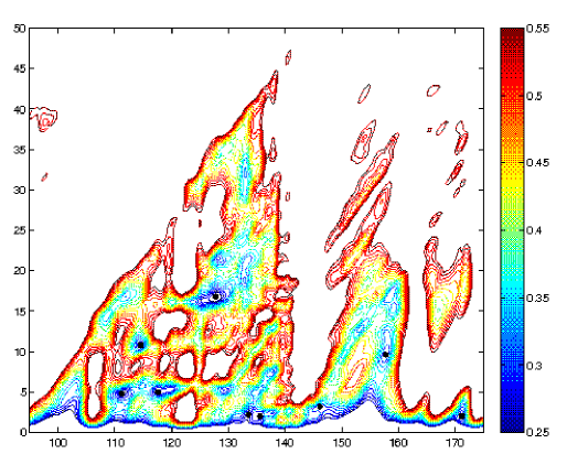
Figure 1: (Low resolution version for the arXiv) $R(t,T)$ at $Re=40$ contoured over $t\in[95,175]$ ($x$-axis) and $T\in[thres,50]$ ($y$-axis). The 9 black dots are the guesses identified by the code ($R<R_{thres}$) over this time interval. All except one (the last dot at $t\approx 171$) subsequently converged to exact solutions - the 4 dots for $t<130$ to a periodic orbit with period 5.3807 ($P1$ in Table 2) and the next 4 dots with $t\in[130,160]$ to a TW ($T1$ in Table 2) with phase speed $c=0.0198$ ($R$ values above 0.55 are not drawn/coloured for clarity.

3.3 UPO extraction method: Newton-GMRES-Hookstep

Once a near-recurrence has been found by the above stated criterion, we then attempted to find if an exact recurrent flow was lurking nearby in phase space. This required a high-dimensional root finding algorithm acting on a state vector which completely specifies the velocity field

$$\mbox{\boldmath$x$}=\left[\begin{array}[]{c}{\bf\Omega}\\ s\\ T\end{array}\right]$$ (24)

and contains information about the potential recurrence (${\bf\Omega}$ is a vector containing the scalars $\Omega_{jl}$ arranged in some fashion). The shift $s$ is included since it can be adjusted continuously whereas the discrete shift $m$ cannot and therefore is pre-set. To set up the Newton-Raphson algorithm (and we follow the excellent description in Viswanath 2009), it is convenient to define the infinitesimal generators $\mathsfi{T}_{x}$ and $\mathsfi{T}_{y}$ of translations in $x$ and $y$ respectively

$$\mathsfi{T}_{x}\,\omega(x,y,t) \rightarrow \frac{\partial\omega}{\partial x}=\sum^{N_{y}/3-1}_{-N_{y}/3}\sum^{N_{x}/3-1}_{-N_{x}/3}i\alpha j\Omega_{jl}(t)e^{i(\alpha jx+ly)},$$

$$\mathsfi{T}_{y}\,\omega(x,y,t) \rightarrow \frac{\partial\omega}{\partial y}=\sum^{N_{y}/3-1}_{-N_{y}/3}\sum^{N_{x}/3-1}_{-N_{x}/3}il\Omega_{jl}(t)e^{i(\alpha jx+ly)}$$

as they act in spectral space

$$\mathsfi{T}_{x}\,{\bf\Omega}\rightarrow{\bf\Omega_{x}}\quad{\rm and}\quad\mathsfi{T}_{y}\,{\bf\Omega}\rightarrow{\bf\Omega_{y}}$$ (25)

where each element $\Omega_{jl}$ of ${\bf\Omega}$ is mapped to $i\alpha j\Omega_{jl}$ in ${\bf\Omega_{x}}$ and $il\Omega_{jl}$ in ${\bf\Omega_{y}}$. Then, in spectral space the recurrence condition (22) becomes

$${\bf F}({\bf\Omega}_{0},s,T;m):=\exp(s\mathsfi{T}_{x}+\mbox{$\frac{1}{2}$}\pi m\mathsfi{T}_{y}){\bf\hat{\Omega}}({\bf\Omega}_{0},T)-{\bf\Omega}_{0}={\bf 0}$$ (26)

where ${\bf\Omega}_{0}={\bf\Omega}(t)$ and ${\bf\hat{\Omega}}={\bf\Omega}(t+T)$. If $\mbox{\boldmath$x$}_{0}=({\bf\Omega}_{0},s_{0},T_{0})^{T}$ is an initial guess for a solution, then a better (next) guess $\mbox{\boldmath$x$}_{0}+\delta\mbox{\boldmath$x$}_{0}=({\bf\Omega}_{0}+\delta{\bf\Omega},s_{0}+\delta s,T_{0}+\delta T)^{T}$ is given by

$$\frac{\partial{\bf F}}{\partial{\bf\Omega}_{0}}{\bf\delta}{\bf\Omega}+\frac{\partial{\bf F}}{\partial s}\delta s+\frac{\partial{\bf F}}{\partial T}\delta T=-{\bf F}({\bf\Omega}_{0},s_{0},T_{0};m)$$ (27)

These are $\dim({\bf\Omega})$ equations for $\dim({\bf\Omega})+2$ unknowns. The extra two equations come from removing the degeneracy associated with these translational symmetries (the system is invariant under $(x,t)\rightarrow(x+s,t+T)$). This can be done by imposing that ${\bf\delta}{\bf\Omega}$, has no component which shifts the solution infinitesimally in the $x$-direction or the $t-$direction (i.e. just redefines the time origin of the flow). The Newton-Raphson problem is then to solve

$$\left[\begin{array}[]{c|c|c}\ddots&\vspace{0.0cm}\vdots&\vspace{0.0cm}\vdots\\ \hskip 28.45274pt{\displaystyle\frac{\partial{\bf\hat{\Omega}_{s}}}{\partial{\bf\Omega}_{0}}}-{\bf I}&\mathsfi{T}_{x}{\bf\hat{\Omega}_{s}}&{\displaystyle\frac{\partial{\bf\hat{\Omega}_{s}}}{\partial T}}\\ \hskip 56.9055pt\ddots&\vdots&\vdots\\ \hline\cr\cdots\quad(\mathsfi{T}_{x}{\bf\Omega}_{0})^{T}\quad\cdots&0&0\\ \hline\cr\cdots\quad{\displaystyle\frac{\partial{\bf\Omega}_{0}}{\partial t}^{T}}\quad\cdots&0&0\end{array}\right]\left[\begin{array}[]{c}\vdots\\ \\ \vspace{0.25cm}\delta{\bf\Omega}\\ \vdots\\ \\ \delta s\\ \\ \\ \delta T\end{array}\right]=-\left[\begin{array}[]{c}\vdots\\ \\ \vspace{0.25cm}{\bf F}({\bf\Omega}_{0},s_{0},T_{0};m)\\ \vdots\\ \\ 0\\ \\ \\ 0\end{array}\right]$$ (28)

where ${\bf\hat{\Omega}_{s}}:=\exp(s\mathsfi{T}_{x}+\mbox{$\frac{1}{2}$}\pi m\mathsfi{T}_{y}){\bf\hat{\Omega}}$ is the ‘back-shifted’ final state and ${\bf I}$ is the $\dim({\bf\Omega})\times\dim({\bf\Omega})$ identity matrix. This is now in the standard form ${\bf A}{\boldsymbol{\delta}{\bf x}}={\bf b}$ with only the Jacobian matrix $\partial{\bf\hat{\Omega}_{s}}/\partial{\bf\Omega}$ not straightforward to evaluate ($\partial{\bf\hat{\Omega}_{s}}/\partial T$ and $\partial{\bf\Omega}_{0}/\partial t$ are found by substituting ${\bf\hat{\Omega}_{s}}$ or ${\bf\Omega}_{0}$ into the Navier-Stokes equations).

Typically, the size of the matrix ${\bf A}$ is too large to store explicitly let alone attempt to solve ${\bf A}{\boldsymbol{\delta}{\bf x}}={\bf b}$ directly. As a result, the only way to proceed is iteratively and GMRES (Saad & Schultz 1986) is convenient (see the excellent description by Trefethen & Bau 1997). Here only the effect of ${\bf A}$ on an arbitrary vector is needed. The effect of the troublesome Jacobian can be handled easily by a forward difference approach since

$$\frac{\partial{\bf\hat{\Omega}_{s}}}{\partial{\bf\Omega}_{0}}{\bf y}\approx\frac{{\bf\hat{\Omega}_{s}}({\bf\Omega}_{0}+\epsilon{\bf y})-{\bf\hat{\Omega}_{s}}({\bf\Omega}_{0})}{\epsilon}$$ (29)

where $\epsilon$ is chosen such that $||\epsilon{\bf y}||=10^{-7}||{\bf\Omega}_{0}||$ which balances truncation error with round-off error using double precision arithmetic and $||\cdot||$ is the Euclidean norm (using a more-physically orientated norm is clearly an interesting direction awaiting exploration).

Straight Newton-GMRES is typically not good enough as guesses are usually not in the region where linearisation holds sufficiently well and divergence to infinity is commonplace. Instead it proves useful to modify the approach to incorporate a trust region. Following Viswanath (2007, 2009), we use the ‘hook-step’ method (Dennis & Schnabel 1996 §6.4.1) which can be easily built on top of the GMRES process. Exactly how the approach is implemented can vary and we adopt what looks to be slightly different algorithm to Viswanath (2007, 2009) in which GMRES is used first to derive an approximate solution to ${\bf A}{\boldsymbol{\delta}{\bf x}}={\bf b}$ before this ‘solution’ ${\boldsymbol{\delta}{\bf x}}$ is moved into the trust region. The advantage of this is there is a clear convergence criterion that can be imposed to terminate the initial GMRES algorithm. Before stating this, it’s worth first briefly describing the GMRES algorithm itself which is based upon a simple idea. The GMRES algorithm for solving ${\bf A}{\boldsymbol{\delta}{\bf x}}={\bf b}$ at iteration $n$ approximates ${\boldsymbol{\delta}}{\bf x}$ by the vector ${\boldsymbol{\delta}}{\bf x}_{n}$ in the Krylov space ${\cal K}_{n}:=\langle\,{\bf b},{\bf Ab},{\bf A^{2}b},\ldots,{\bf A^{n-1}b}\,\rangle$ that minimises the norm of the residual

$$\|{\bf A}{\boldsymbol{\delta}{\bf x}_{n}}-{\bf b}\|$$ (30)

(Trefethen & Bau 1997). For numerical stability, an orthonormal basis for ${\cal K}_{n}$ is constructed using a Gram-Schmidt-style iteration as follows

$$\mbox{\boldmath$q$}_{1}=\frac{{\bf b}}{\|{\bf b}\|},\qquad\tilde{\mbox{\boldmath$q$}}_{i+1}={\bf A}\mbox{\boldmath$q$}_{i}-\sum_{j=1}^{i}\mbox{\boldmath$q$}_{j}\frac{\mbox{\boldmath$q$}_{j}^{T}{\bf A}\mbox{\boldmath$q$}_{i}}{\|\mbox{\boldmath$q$}_{j}\|^{2}}\qquad\mbox{\boldmath$q$}_{i+1}=\tilde{\mbox{\boldmath$q$}}_{i+1}/\|\tilde{\mbox{\boldmath$q$}}_{i+1}\|\qquad i\in{1\ldots,n-1}$$ (31)

so that if ${\bf Q}_{n}$ is the matrix with columns $\mbox{\boldmath$q$}_{1},\mbox{\boldmath$q$}_{2},\ldots,\mbox{\boldmath$q$}_{n}$, then ${\bf AQ}_{n}={\bf Q}_{n+1}{\bf H}_{n+1,n}$ where ${\bf H}_{n+1,n}$ is the upper $(n+1)\times n$ left section of an upper Hessenberg matrix generated by the basis orthonormalisation (Trefethen & Bau 1997, p252). With this basis the solution ${\boldsymbol{\delta}{\bf x}_{n}}={\bf Q}_{n}{\bf y}_{n}$ (where ${\bf y}_{n}$ is an $n$-vector) minimises $\|{\bf Q}_{n+1}{\bf H}_{n+1,n}{\bf y}_{n}-{\bf b}\|$ ($N$ equations and $n$ unknowns) or equivalently $\|{\bf H}_{n+1,n}{\bf y}-\|{\bf b}\|{\bf\hat{e}_{1}}\|$ ($n+1$ equations and $n$ unknowns) since the only non-zero entry in ${\bf Q}_{n+1}^{T}{\bf b}$ is the first entry. This can be accomplished by a singular value decomposition (SVD) of ${\bf H}_{n+1,n}$ into ${\bf U}_{n+1}{\bf D}{\bf V}_{n}^{T}$ (where ${\bf U}_{n+1}$ and ${\bf V}_{n}$ are orthonormal matrices and ${\bf D}$ is an $(n+1)\times n$ diagonal matrix with a zeroed bottom row) through straightforwardly solving the first $n$ equations ${\bf D}{\bf z}_{n}={\bf p}_{n+1}:=||{\bf b}||{\bf U}_{n+1}^{T}{\bf\hat{e}_{1}}$ followed by ${\bf V}^{T}{\bf y}_{n}={\bf z}_{n}$ and then ${\boldsymbol{\delta}{\bf x}_{n}}={\bf Q}_{n}{\bf y}_{n}$. The modulus of the remaining unbalanced component $p_{n+1}(n+1)$ then gives the minimum value or residual. The iterations are continued until

$$\frac{\|{\bf A}{\boldsymbol{\delta}{\bf x}_{n}}-{\bf b}\|}{\|{\bf b}\|}=\frac{\|{\bf D}{\bf z}_{n}-{\bf p}_{n+1}\|}{\|{\bf p}_{n+1}\|}=\frac{|p_{n+1}(n+1)|}{\|{\bf p}_{n+1}\|}\leq tol$$ (32)

where $tol$ is a small number typically chosen in the range $10^{-4}$ to $10^{-2}$ (the majority of the computations reported here were obtained using a value of $10^{-3}$). If $\|{\bf F}({\bf x}+{\boldsymbol{\delta}{\bf x}_{n}})\|$ is not smaller than $\|{\bf F}({\bf x})\|$ or more specifically not well predicted by the linearisation around ${\bf x}$ i.e. $\|{\bf F}({\bf x})+{\bf A}{\boldsymbol{\delta}{\bf x}_{n}}\|$, then the approximate solution of the linearised problem is transformed back to a smaller trust region where the linearised problem is valid. This is done by adding the constraint $\|{\boldsymbol{\delta}{\bf x}_{n}}\|\leq\Delta$ or equivalently $\|{\bf y}_{n}\|\leq\Delta$ to the GMRES minimisation (30): this is the hook step. The beauty of this adjustment is that it is a very natural modification of the GMRES approximate solution since the (innermost) problem for ${\bf z_{n}}$ is then

$${\rm min}\|{\bf D}{\bf z}_{n}-{\bf p}_{n+1}\|\qquad{\rm s.t.}\quad\|{\bf y}_{n}\|=\|{\bf z_{n}}\|\leq\Delta$$ (33)

Constructing the Lagrangian

$${\cal L}:=({\bf D}{\bf z}_{n}-{\bf p}_{n+1})^{2}+\mu({\bf z}_{n}^{2}+\beta^{2}-\Delta^{2})$$ (34)

where $\mu$ is a Lagrange multiplier imposing the trust region constraint, leads to the minimisation equations

$$2d(i)(d(i)z_{n}(i)-p_{n+1}(i))+2\mu z_{n}(i) = 0$$ (35)

$$2\mu\beta = 0$$ (36)

$${\bf z}_{n}^{2}+\beta^{2}-\Delta^{2} = 0$$ (37)

where $d_{i}$ is the $i$th diagonal element of ${\bf D}$. The solution to this is

$$z_{n}(i):=\frac{p_{n+1}(i)d_{i}}{d_{i}^{2}+\mu}\qquad 1\leq i\leq n$$ (38)

with either $\mu=0$ as $\|{\bf z}_{n}\|<\Delta$ (the original GMRES solution) or $\mu\neq 0$ chosen so that $\|{\bf z}_{n}\|=\Delta$ (in practice $\mu$ is just increased until $\|{\bf z}_{n}\|<\Delta$). An acceptable solution ${\boldsymbol{\delta}{\bf x}_{n}}$ is signalled by

$${\bf F}({\bf x}+{\boldsymbol{\delta}}{\bf x}_{n})\leq{\bf F}({\bf x})+c{\bf A}{\boldsymbol{\delta}}{\bf x}_{n}$$ (39)

where some value of $c\in(0,0.5)$ is chosen (eqn 6.4.14, Dennis & Schnabel 1996: we took the least demanding value of $c=0$). If this does not hold, $\Delta$ is decreased and the hook step repeated until it is. Depending on how easily this improvement condition is met, the trust region may be relaxed (e.g. if linearisation holds well - ${\bf F}({\bf x}+{\boldsymbol{\delta}}{\bf x}_{n})\approx{\bf F}({\bf x})+{\bf A}{\boldsymbol{\delta}}{\bf x}_{n}$) or not for subsequent Newton steps.

This algorithm can be readily extended to perform solution branch continuation: see appendix A. Furthermore, since we know how to calculate the action of the Jacobian on any vector (see (29), the linear stability of an exactly recurrent flow can also be readily found using the Arnoldi technique (e.g. using ARPACK to extract extremal eigenvalues).

3.4 Testing

The modified (Crank-Nicholson+Heun) time-stepping code was thoroughly validated against the well-tested Leapfrog+filter code developed by Bartello & Warn (1996). The Newton-GMRES-Hookstep algorithm developed on top of this was tested by attempting to converge onto a known periodic orbit. This orbit was originally found by tracing bifurcations up from the basic state. For $n=4$, the 1D basic state becomes linearly unstable at $Re=9.9669$ for disturbances $2\pi$-periodic in $x$ giving rise to a steady 2D state which is ${\cal R}$-symmetric. This state loses stability to a stable periodic orbit within the ${\cal R}$-symmetric subspace for $30<Re<31$ before this orbit becomes unstable at $Re\gtrsim 32$ through a torus bifurcation. The periodic orbit at $Re=31$ was easily found by time-stepping within the ${\cal R}$-symmetric subspace yet is unstable to ${\cal R}$-asymmetric disturbances in the full unrestricted space. Having such an orbit to experiment with was invaluable for building up confidence in the code and some feel for how the tolerances of the algorithm should be set (e.g. $tol$ in (32)).

4 Results

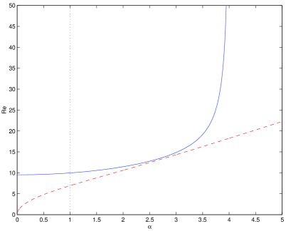
Figure 2: The energy stability Reynolds number $Re_{E}$ (red dashed line) and the linear instability Reynolds number $Re_{lin}$ (blue solid line) for $\sin 4y\boldsymbol{\hat{x}}$ forcing over the torus $[0,2\pi/\alpha]\times[0,2\pi]$. Note that $Re_{lin}\rightarrow\infty$ as $\alpha\rightarrow 4$ so the domain is squeezed down to $[0,\pi/2]\times[0,2\pi]$. The dotted line at $\alpha=1$ is the present case ($Re_{E}=6.8297$ and $Re_{lin}=9.9669$). $Re_{E}\rightarrow 0$ and $Re_{lin}\rightarrow 8\sqrt[4]{2}\approx 9.5137$ as $\alpha\rightarrow 0$.

Figure 3: The normalised dissipation $D/D_{lam}$ (blue solid line with dots) and fractional fluctuation kinetic energy $E_{t}/E$ (red dotted line connecting dots) to illustrate how the flow changes with $Re$. The first bifurcation at $Re_{lin}=9.9669$ is steady so $D/D_{lam}$ decreases below 1 but $E_{t}/E$ remains 0 until time-dependent flows appear at around $Re=15$. Curves were generated by using a random initial condition, running for 500 time units and then calculating averages over the next 1000 time units. This produces a unique average except over the interval $15\lesssim Re\lesssim 23$ where there is some metastability as shown. Inset: $Re^{1/2}D$ (upper blue line) and $3Re^{-2/5}E^{1/2}$ (lower thick red line) against $Re$ on a log scale showing the apparent start of the asymptotic regime $D\sim Re^{-1/2}$ and $U:=\sqrt{2E}\sim Re^{2/5}$. The downward sloping lowest line shows $U/Re^{1/2}$ for comparison.

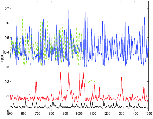
Figure 4: The normalised dissipation $D(t)/D_{lam}$ vs $t\in[500,1500]$ for Re=$22$ (two different initial conditions: top solid blue & green dashed lines), $Re=40$ (second lowest red line) and $Re=100$ (lowest black line). $Re=22$ shows chaotic saddle behaviour with one trajectory seemingly dropping out back randomly to the travelling wave T1 (stable at $Re=22$).

Figure 5: A time sequence of vorticity plots at $Re=40$ (upper) and $Re=100$ (lower) over the $2\pi\times 2\pi$ domain. Time difference between plots is 1 time unit and 10 contours are drawn between the maximum (white/light) and minimum values (red/dark) of the perturbation vorticity $-10.25\leq\omega\leq 8.6$ at $Re=40$ and $-18.4\leq\omega\leq 20.3$ at $Re=100$.

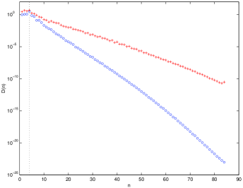
Figure 6: The enstrophy spectrum for the rightmost snapshots in figure 5 at $Re=40$ (blue circles) and $Re=100$ (red crosses) $D(n):=\sum_{n-\mbox{$\frac{1}{2}$}\leq\sqrt{j^{2}+l^{2}}<n+\mbox{$\frac{1}{2}$}}|\Omega_{jl}|^{2}$ for $n=1,2...85$: recall definition (21 with $\alpha=1$) (e.g. there are 264 and 516 wavenumbers included for $n=40$ and $84$ respectively). The energy spectrum $E(n)\approx D(n)/n^{2}$ has a steeper drop off. The dotted line indicates the wavenumber of energy injection.

4.1 Flow Orientation

2D Kolmogorov flow is linearly unstable at a comparatively low $Re$ which depends strongly on the imposed periodicity in the forcing direction: see figure 2. For the domain studied here ($\alpha=1$), disturbances to the base flow (15) fail to decay monotonically at $Re_{E}=6.8297$ and then start to grow exponentially at $Re_{lin}=9.9669$. Figure 3 shows that this initial bifurcation is to a steady flow ($D/D_{lam}<1$ and $E_{t}/E=0$) until $Re\approx 15$ whereupon time dependence appears. For $15\lesssim Re\lesssim 23$, some metastability is noticed which is illustrated in figure 4 at $Re=22$ for two different initial conditions. One leads to a chaotic-looking dissipation signal across the time interval $[500,1500]$ whereas the other drops out of this chaotic state at just over t=1000 to converge on a stable travelling wave solution (later named T1). Beyond $Re\approx 23$, the chaotic state presumably becomes an attractor or the probability of dropping out of this state becomes so small that it is not picked up over the time windows studied ($10^{3}$ units here and $10^{5}$ later). Finally, an asymptotic regime is approached for $Re\gtrsim 50$. The preliminary calculations performed here for $100<Re<200$ tentatively support the asymptotic scaling laws $D\sim Re^{-1/2}$ and $U:=\sqrt{2E}\sim Re^{2/5}$ although the noisy data clearly warrants much longer time averaging to confirm this.

Given this general flow behaviour, we chose to concentrate on analysing the flow at $Re=40$ (approaching the asymptotic regime), and three values, $Re=60,80$ and $100$, which get deeper into the asymptotic regime. Figures 4 and 5 give an idea of the temporal and spatial scales in the flow at the two extremes, $Re=40$ and $Re=100$, of our study. Both indicate a hierarchy of temporal and spatial scales (which broaden with $Re$) indicative of 2D turbulence. Figure 6 confirms that the flows studied for $Re\leq 100$ are well-resolved: there is 10 orders of drop off in the enstrophy spectrum in the most demanding case ($Re=100$) for the $256^{2}$ resolution used throughout this work.

4.2 Finding recurrent structures

A standard hunt for recurrent flows involved integrating the flow from random initial conditions for a period of $10^{5}$ time units. Initially, $R_{thres}$ was set at 0.15 for three runs at $Re=40$ (labelled $a$,$b$ and $c$ in Table 1) which produced only 9, 7 and 13 guesses respectively. Relaxing $R_{thres}$ to 0.3 (run $d$), however, produced 885. This threshold value proved adequate at $Re=60$ (nearly 300 near-recurrences detected over runs $e$,$f$ and $g$) but had to be further relaxed to $0.35$ at $Re=80$ and $0.4$ for $Re=100$: see Table 1. Unfortunately, it was noticed after these (Series A) runs had been completed and the guesses tested for convergence that only $s=m=0$ shifts had been searched over. So the runs were repeated (Series B runs $o$, $p$, $q$ and $r$) searching specifically for recurrences which selected either $s\neq 0$ and/or $m\neq 0$ to minimise $R$. This was done to indicate the frequency of observing strictly periodic near-recurrences and relative periodic near-recurrences.

The initial trawl for near-recurrences took a few weeks (each case run on a Xeon X5670 processor) with the DNS code slowed considerably by the need to search for near-recurrences every $0.1$ or $0.2$ units in time (which is anything from 20 to 100 numerical time steps). The more time-consuming activity, however, was attempting to converge the near-recurrent guesses to exact solutions. Adopting fairly conservative limits for the Newton-GMRES-Hookstep procedure - maximum period considered was 100, maximum number of Newton, GMRES and Hook steps were 75, 500 and 50 respectively - typically lead to run times of a couple of months for each of the $Re=60,80$ and $100$ runs. The data for $Re=40$ had to be subdivided 12 ways to make the process manageable. These numbers make it clear why a very efficient DNS code was important for this work.

Table 1 also indicates the conversion rate of near-recurrences guesses to exactly recurrent solutions. There is considerable duplication of such solutions so that a much smaller set of distinct recurrent structures is obtained.

	Run	$R_{thres}$	dt	duration	# of guesses	# of convergences
Series A	$(s=m=0)$
$Re=40$	a	0.15	0.005	$10^{5}$	9	5
	b	0.15	0.005	$10^{5}$	7	3
	c	0.15	0.005	$10^{5}$	13	5
	d	0.30	0.005	$10^{5}$	885	553
$Re=60$	e	0.30	0.003	$10^{5}$	102	64
	f	0.30	0.003	$10^{5}$	104	67
	g	0.30	0.003	$10^{5}$	78	58
$Re=80$	h	0.35	0.0025	$10^{5}$	53	31
	i	0.35	0.0025	$10^{5}$	60	37
	j	0.35	0.0025	$10^{5}$	41	25
$Re=100$	l	0.4	0.002	$10^{5}$	75	34
	m	0.4	0.002	$10^{5}$	91	33
	n	0.4	0.002	$10^{5}$	93	42
Series B	$(s\neq 0$ or $m\neq 0)$
$Re=40$	o	0.30	0.005	$10^{5}$	1223	540
$Re=60$	p	0.30	0.003	$3\times 10^{5}$	163	7
$Re=80$	q	0.35	0.0025	$3\times 10^{5}$	66	15
$Re=100$	r	0.4	0.002	$3\times 10^{5}$	84	12

Table 1: DNS data used to extract equilibria, travelling waves, periodic orbits and relative periodic orbits at $Re=40,60,80$ and $100$. The value of $R_{thres}$ cannot be set too ambitiously. Run d yielded all the solutions thrown up by runs a,b and c combined.

	UPO	frequency	$c$	$T$	$-s$	$-m$	$N$	$\sum_{j=1}^{N}\Re e(\lambda_{j})$ ( max$\,\Re e(\lambda_{j}$) )
$Re=40$	E1	$\geq$ 261				0	9	1.296(0.249)
	T1	127	0.0198			0	4	0.142(0.068)
	T2	1	0.0096			0	4	1.227(0.454)
	P1	143		5.380		0	7	0.570(0.191)
	P2	6		2.830		0	5	0.742(0.223)
	P3	2		2.917		0	7	0.992(0.236)
	R1	1		56.677	0.092	0	3	0.156(0.077)
	R2	1		25.401	0.199	0	5	0.254(0.123)
	R3	1		54.280	0.200	0	3	0.195(0.108)
	R4	1		6.720	0.106	0	8	0.870(0.343)
	R5	1		23.780	0.022	0	4	0.376(0.156)
	R6	4		20.808	0.060	0	3	0.258(0.172)
	R18	1		37.233	0.270	0	5	0.242(0.165)
	R19			12.207	0.243	0	2	0.141(0.070)
	R20			16.586	5.827	1	4	0.289(0.103)
	R21			17.470	5.765	3	5	0.348(0.143)
	R22			19.723	0.222	0	4	0.297(0.172)
	R23			19.762	0.513	0	4	0.302(0.127)
	R24			19.779	6.035	0	5	0.292(0.202)
	R25			20.201	5.898	3	6	0.380(0.138)
	R26			20.385	1.334	2	7	0.714(0.270)
	R27			20.632	5.871	3	4	0.365(0.127)
	R28			20.885	5.987	1	4	0.360(0.121)
	R29			20.909	0.306	1	5	0.380(0.124)
	R30			21.310	5.694	0	5	0.330(0.100)
	R31			21.725	5.799	0	3	0.319(0.133)
	R32			22.560	0.006	1	4	0.283(0.096)
	R33			22.617	5.660	0	5	0.478(0.156)
	R34			23.157	0.265	0	3	0.260(0.113)
	R35			23.417	5.936	3	4	0.489(0.183)
	R36			24.465	6.010	3	4	0.358(0.191)
	R37			25.870	0.182	0	3	0.272(0.122)
	R38			25.934	0.227	0	4	0.263(0.125)
	R39			27.138	6.248	0	4	0.391(0.107)
	R40			28.817	5.971	0	5	0.238(0.116)
	R41			32.541	0.349	1	4	0.224(0.153)
	R42			34.316	5.886	0	5	0.163(0.120)
	R43			34.530	5.742	0	3	0.220(0.134)
	R44			34.917	-0.059	3	4	0.325(0.139)
	R45			36.549	6.027	3	3	0.183(0.118)
	R46			36.627	0.197	3	4	0.202(0.139)
	R47			36.812	5.648	0	3	0.155(0.074)
	R48			37.079	6.103	0	4	0.171(0.134)
	R49			37.233	0.270	0	3	0.241(0.165)
	R50			37.698	3.499	1	6	0.477(0.146)
	R51			39.368	6.070	0	5	0.192(0.098)
	R52			39.619	0.380	0	5	0.242(0.067)
	R53			41.400	5.806	0	4	0.176(0.081)
	R54			49.645	6.054	3	4	0.160(0.065)
	R55			53.073	6.031	0	4	0.189(0.105)

Table 2: All the invariant sets found directly from turbulent DNS data (from series A above the separating blank line and from series B below). ‘Frequency’ is the number of times the solution was extracted (Series A runs). There is one steady Equilibrium, $c$ is the phase speed of the Travelling waves found, $T$ is the Period of periodic and Relative periodic orbits which also either have a shift $s$ and/or shift $m$. $N$ is the number of unstable directions and $\sum_{j=1}^{N}\Re e(\lambda_{j})$ the sum of the real parts of all the unstable eigenvalues.

	UPO	frequency	$c$	$T$	$-s$	$-m$	$N$	$\sum_{j=1}^{N}\Re e(\lambda_{j})$ ( max$\,\Re e(\lambda_{j}$) )
$Re=60$	E1	4				0	14	5.053(0.858)
	T1	high	0.0019			0	4	0.139(0.064)
	T3	high	0.0124			0	17	3.377(0.684)
	T4	1	0.0082			0	3	0.257(0.178)
	R7	high		2.472	0.036	0	9	0.911(0.214)
	R8	1		1.638	0.022	0	14	2.903(0.681)
	R56			16.326	0.588	2	6	0.609(0.139)
	R57			17.909	5.802	0	7	0.805(0.169)
	R58			20.546	0.659	2	8	0.529(0.168)
$Re=80$	T1	high	0.0115			0	6	0.360(0.105)
	T3	8	0.0154			0	21	5.588(0.958)
	T5	3	0.0831			0	20	4.183(0.658)
	R7	10		2.299	0.054	0	13	1.326(0.181)
	R8	2		1.705	0.028	0	18	4.318(1.105)
	R9	1		2.150	0.032	0	19	3.987(1.026)
	R10	1		1.280	0.020	0	20	5.310(0.878)
	R11	1		2.443	0.031	0	10	0.704(0.277)
	R12	1		2.095	0.034	0	11	3.083(1.004)
	R13	1		15.285	0.181	0	8	0.409(0.131)
	R59			15.667	0.397	1	11	0.949(0.176)
	R60			16.071	0.462	1	11	1.136(0.248)
$Re=100$	T1	high	0.0155			0	10	0.646(0.122)
	T3	7	0.0179			0	25	6.491(1.042)
	T4	5	0.0118			0	3	0.684(0.370)
	T5	6	0.0691			0	28	6.238(0.689)
	P4	1		1.185		0	16	7.376(1.201)
	R7	4		1.971	0.030	0	15	1.933(0.326)
	R11	3		2.262	0.001	0	9	0.905(0.385)
	R12	1		1.902	0.029	0	14	3.953(1.244)
	R14	5		4.526	0.071	0	8	0.428(0.105)
	R15	2		1.984	0.122	0	16	3.110(0.556)
	R16	2		1.938	0.121	0	6	0.945(0.270)
	R17	1		3.827	0.008	0	16	2.894(0.818)
	R61	1		1.344	0.090	0	21	4.997(0.476)

Table 3: All the invariant sets found directly from turbulent DNS data (from series A above the separating blank line and from series B below: none were found at $Re=100$ in the series B runs despite the numerical gap between $R17$ and $R61$). ‘Frequency’ is the number of times the solution was extracted. Solutions listed under each $Re$ indicate those actually extracted at that $Re$ - hence multiple entries. ‘Frequency’ is the number of times the solution was extracted (Series A runs). There is one steady Equilibrium, $c$ is the phase speed of the Travelling waves found, $T$ is the Period of periodic and Relative periodic orbits which also either have a shift $s$ and/or shift $m$. $N$ is the number of unstable directions and $\sum_{j=1}^{N}\Re e(\lambda_{j})$ the sum of the real parts of all the unstable eigenvalues.

4.3 Recurrent structures found

4.3.1 Re=40

Table 2 lists the recurrent structures found at $Re=40$. The equilibrium flow $E1$ (see figure 7), which was found many times in the series A runs, corresponds to the ${\cal R}$-symmetric steady state which bifurcates off the basic solution at $Re=9.9669$ as shown in figure 3. $E1$ loses stability at about $Re=15$ to the travelling wave $T1$ or later via $P1$ in the ${\cal R}$-symmetric subspace for a $Re\in(30,31)$ ($P2$ which is ${\cal R}$-symmetric and $P3$ which is not bifurcate at yet higher $Re$ from $E1$). All three flows, $E1$, $P1$ and $T1$ are found to be repeatedly visited by the (series A) DNS indicating the strong influence of the ${\cal R}$-symmetric subspace on the ‘turbulent’ dynamics despite them all being unstable (e.g. $E1$ has 9 unstable directions at $Re=40$; see Table 2). However, a further 47 recurrent flows were also identified from the DNS: another travelling wave $T2$, two further periodic orbits $P2$ and $P3$, and 44 relative periodic orbits, $R1-R6$ and $R18-R55$ (note all have a non-zero shift $s$ and some also a non-zero integer $m$). A priori, we expected to find mainly small period recurrent structures due to the method of extraction. Longer periods mean more time for the turbulent trajectory to diverge away from the unstable recurrent flow and hence a higher probability for a) the episode to escape detection as a nearly recurrent flow and b) even if detected, for GMRES to fail to converge due to the quality of the initial approximation. This seems borne out by the periodic orbits found but not for the relative period orbits where the majority have a period over 20 and some over 50 time units. That such long period structures exist and were ‘extractable’ from the DNS frankly was a surprise and begs the question whether our ‘long’ runs of $10^{5}$ time units (now known to be only a factor of $O(1000)$ longer than some recurrent flows) were actually really long enough to capture all the structures possible. This issue will be raised again below.

With so many recurrent flows found, it becomes impractical to display and characterise each flow separately. Table 2 lists some key characteristics along with their stability information (all are unstable but none with more than 9 unstable directions out of 22,428 possible directions). One useful projection used by Kawahara & Kida (2001), however, is the ‘energy out ($D(t)$) verses energy in ($I(t)$)’ plot which is shown in figure 8 (both quantities normalised by $D_{lam}$). The line $D=I$ corresponds to dissipation exactly balancing energy input which has to be the case over all times for equilibria and travelling waves (which are just equilibria in an appropriate Galilean frame): these are therefore just points on this line in this plot. Figure 8 shows how a representative subset of these recurrent flows look when compared with the joint dissipation-input probability density function (pdf) of the DNS. The darkest shading makes it clear that the DNS stays predominantly in the region ${0.055\,<\,I/D_{lam}\,<\,0.115,\,0.06\,<\,D/D_{lam}\,<\,0.11}$. The recurrent flows shown are also dominantly concentrated in this region although there are two relative periodic orbits shown - $R26$ and $R50$ - which have large dissipation episodes (it’s worth emphasizing that the basic state would be represented by the point (1,1) in this plot so the turbulent flow adopts a much reduced dissipative state). Since this $D$ verses $I$ plot is such a drastic projection of the dynamics, the fact that two flows look close there doesn’t necessarily mean they are close in the full phase space. However, because all the recurrent flows discussed here have been extracted from turbulent DNS, this conclusion nevertheless seems reasonable.

In figure 9 we focus on one typical ‘embedded’ relative periodic orbit $R25$ which stays within the central region of the DNS joint pdf. There is a clear temporal cycle where the energy input increases (exceeding the dissipation) and then decreases (now exceeded by the dissipation). Plotting the associated vorticity fields over this cycle - figure 10 - shows the character of the flow. At the dissipation low point (time 17 in figures 9 and 10), the vorticity is concentrated into weak $y$-aligned patches which are separated from each other whereas at the high dissipation point (time 8), the vorticity seems to be undergoing a shearing episode with only one stronger vortex recognisable. These two extremes bear more than a passing resemble to either $T1$ ($D/D_{lam}=0.071$) or $T2$ (0.071) and $E1$ (0.102) respectively suggesting that $R25$ is probably a closed trajectory linking their neighbourhoods. $R50$, in contrast, undergoes a large high dissipation excursion as shown more completely in figure 11. The associated vorticity fields - see figure 12 - show similar structures to $R25$ when in the same part of $(I,D)$ space (compare t=5 for $R25$ with t=0 for $R50$, and t=15 for $R25$ and t=31 for $R50$) but $R50$ exhibits intense shearing too and vortex break-up at times 5, 8 and 9. $R50$ clearly reflects an important but infrequent aspect of the turbulent dynamics as indicated by the fact that the joint $(D,I)$ pdf of the DNS stretches to such high values of the dissipation. Whether we have extracted enough of such recurrent structures to capture this episodic behaviour is of course a key issue for this study and will be discussed in §5

Figure 13 is an attempt to show more of the recurrent structures found by zooming in on the central dashed box drawn in figure 8. This illustrates the intricacy of most of the flows found - many of the relative periodic orbits trace complicated $D-I$ curves whereas, in contrast, the periodic orbits are simple loops. Another key observation is that some relative periodic orbits look very similar - e.g. $R28$ and $R29$ (and other pairings not shown). This, of course, resonates with the mental picture one has of periodic orbits being dense in a chaotic attractor. In fact, the consecutive numbering of $R28$ and $R29$ indicates that these relative periodic orbits were found concurrently from the DNS confirming their proximity in phase space. Also it is clear than some relative periodic orbits look like merged versions of two shorter orbits (not shown) again consistent with low-dimensional dynamical systems thinking.

Figure 7: The steady solution $E1$ (left) and the travelling waves $T1$ (middle) and $T2$ (right) at $Re=40$. Vorticity is contoured using 15 contours between -7.2 (dark,red) and 12.1 (light,white) (range is $-6.5\leq\omega\leq 12.1$ for $E1$, $-7.2\leq\omega\leq 7.2$ for $T1$ and $-6.8\leq\omega\leq 10.4$ for $T2$).

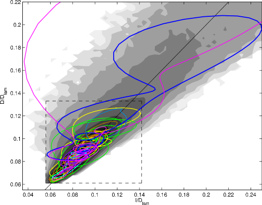
Figure 8: The normalised dissipation $D(t)/D_{lam}$ verses $I/D_{lam}$ for a small collection of the recurrent flows found with the pdf of the DNS turbulence plotted in the background (11 shades at levels $10^{\alpha}$ where $\alpha={-5,-4.5,\ldots,-0.5,0}$). Plotted are $E1$ ($D/D_{lam}=I/D_{lam}=0.102$), $T1$ (0.071), $T2$ (0.070), $P1$, $P2$, $R1-6$, $R18$, $R26$ (large blue orbit) and $R50$ (the even larger magenta orbit). The dashed box is used to show more recurrent structures in figure 13.

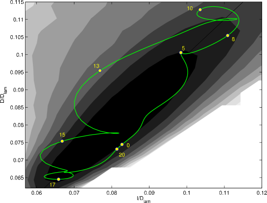
Figure 9: The normalised dissipation $D(t)/D_{lam}$ verses $I/D_{lam}$ for the relative periodic orbit $R25$ at Re=$40$ with the pdf of the DNS turbulence plotted in the background (11 shades at levels $10^{\alpha}$ where $\alpha={-5,-4.5,\ldots,-0.5,0}$). The labels refer to times along the orbit at which snapshots are shown in figure 10.

Figure 10: A time sequence of vorticity plots for $R25$ at $Re=40$ at times (running left to right across the top and then bottom) $t=0,5,8,10,13,15,17,20$ (marked as dots on figure 9). The period is 20.2 so the flow in the bottom right is nearly the same as the top left except for shifts in $x$ and $y$. For all, 15 contours are plotted from -12 to 12.

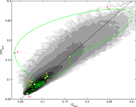
Figure 11: The normalised dissipation $D(t)/D_{lam}$ verses $I/D_{lam}$ for the relative periodic orbit $R50$ at Re=$40$ with the pdf of the DNS turbulence plotted in the background (11 shades at levels $10^{\alpha}$ where $\alpha={-5,-4.5,\ldots,-0.5,0}$). The labels refer to times along the orbit at which snapshots are shown in figure 12.

Figure 12: A time sequence of vorticity plots for $R50$ at $Re=40$ at times (running left to right across the top and then bottom) $t=0,5,8,9,10,26,31,37$ (marked as dots on figure 11). The period is 37.7 so the flow in the bottom right is nearly the same as the top left except for shifts in $x$ and $y$. For all, 15 contours are plotted from -12 to 12.

Figure 13: A sampling of the recurrent structures found at $Re=40$ plotted over the zoom-in box shown in figure 8. Upper left shows $P1$,$P2$,$R2$ and $R4$; Upper right shows $R28$,$R29$ and $R38$; Lower left shows $R19$, $R39$ and $R55$; and lower right shows $R40$, $R48$ and $R53$. In all cases, symbols added to lines are to assist in their distinction and are placed 1 time unit apart to indicate speed of flow.

4.3.2 Re=60, 80 & 100

At higher $Re$, we managed to extract far fewer recurrent flows from the DNS. There are certainly reasons to expect this, most notably that the recurrent flows present should become more unstable and it is therefore harder to find good guesses from the DNS. And there is also the fact that the ‘turbulence’ should explore more of phase space and therefore close visits to simple invariant sets should become rarer. However, the sharp drop in the number of recurrent flows found - see Table 3 - was still a surprise. In keeping with the philosophy of this work, only recurrent flows extracted from the DNS at that $Re$ are listed in Table 3 under the relevant $Re$ heading. This then says nothing about whether a certain recurrent flow found at one $Re$ might not exist at another. To explore this a little, we carried out some branch continuation (see appendix A) on the recurrent flows extracted from the series A DNS while the runs and analysis for the series B DNS were progressing. The results are shown in figure 14 colour coded to group recurrent flows found at the same $Re$ and with black dots indicating branches detected at a given $Re$ (note the rescaled dissipation measure on the ordinate to make the plot clearer). For example, the $T3$ branch is shown as a dashed red line (second red dashed line up from the $Re$ axis) as it was first found at $Re=60$ and it bears three black dots marked at $Re=60,80$ and $100$ as $T3$ was extracted from the DNS at all three $Re$. This type of analysis can indicate the bifurcation structure - e.g. $T3$ clearly bifurcates off a recurrent flow found at $Re=40$ - but is very time-consuming to pursue through to completion as branches can become difficult to continue and interpret (note the number of open circles in figure 14 which indicate where the branch continuation procedure stagnated for some reason). This aside, the overriding impression is one of simple invariant sets proliferating with increasing $Re$. Notably, only two recurrent flows found at $Re=40$ are also extracted from the $Re=60$ DNS - $E1$ (the highest blue line with a dot at $Re=60$) and $T1$. $E1$ seems to lose dyanmical importance for yet higher $Re$ but $T1$ is found for all four $Re$ studied here.

Figure 15 shows the new travelling waves found and figures 16 to 18 the $D-I$ plots where now all the recurrent flows found at the respective $Re$ are marked. Again most sit in the $D-I$ region where the DNS spends the majority of its time although as at $Re=40$ there are some outliers (e.g. $E1$ at $Re=60$, $R8$ at $Re=80$, and $P4$ and $R14$ at $Re=100$). That $R14$ actually appears outside the footprint of the DNS pdf at first looks erroneous but is in fact merely an indication that when the ‘turbulence’ approached $R14$ in phase space, it maintained higher (global) dissipation and energy input than $R14$. This can occur when part of the domain resembles $R14$ while the rest does not and exhibits enhanced dissipation. A good example of this is shown in figure 19 which details the turbulent episode which signalled the presence of $P4$ (left column) alongside the successfully converged periodic orbit $P4$ (right column). Visually, the eye is drawn to the centre of the domain where in both columns an isolated vortex is clearly seen rotating in a clockwise fashion. However, the corners are just as significant in that they also indicate an isolated vortex, yet this is stronger with higher gradients (and hence larger dissipation) for $P4$ than the DNS signal. Plotting the two time sequences on a $D-I$ plot shows $P4$ as a closed loop much higher up the $D=I$ line than the DNS (not shown).

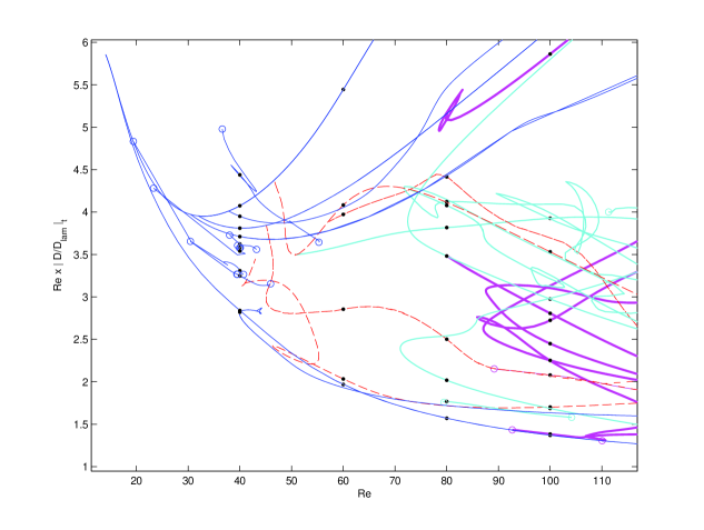
Figure 14: The scaled, time-averaged dissipation $Re\langle D/D_{lam}\rangle_{t}$ verses $Re$ for recurrent flows discovered by the series A runs. Blue thin lines trace recurrent flows found at $Re=40$, red thin dashed lines new recurrent flows found at $Re=60$, thick cyan lines those found at $Re=80$ and very thick magenta lines those at $Re=100$. The black dots identify the subset of solutions which were identified by processing the dns runs at the respective $Re$ as opposed to just being continued up or down from other $Re$ (e.g. there are 6 dots at $Re=60$ corresponding to $E1,T1,T3,T4,R7$ and $R8$: $R56$-$R58$ were discovered in the series B runs, and none of the red dashed lines join dots at $Re=40$). Open circles indicate limits beyond which a solution branch could not be continued. The situation is clearly complicated with solutions seemingly dynamically important at some $Re$ but not at others.

Figure 15: The travelling waves $T3$ (left), $T4$ (middle) and $T5$ (right) at $Re=100$. Vorticity is contoured using 15 contours between -20 (dark,red) and 15 (light,white) (range is $-18.9\leq\omega\leq 8.03$ for $T3$, $-11.5\leq\omega\leq 11.5$ for $T4$ and $-13.7\leq\omega\leq 13.7$ for $T5$).

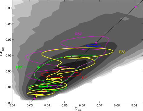
Figure 16: The normalised dissipation $D(t)/D_{lam}$ verses $I/D_{lam}$ for the recurrent flows found at $Re=60$ with the pdf of the DNS turbulence plotted in the background (11 shades at levels $10^{\alpha}$ where $\alpha={-5,-4.5,\ldots,-0.5,0}$). Plotted are $E1$ ($D/D_{lam}=I/D_{lam}=0.091$), $T1$ (0.033), $T3$ (0.068), $T4$ (0.034), $R7$, $R8$, $R56-8$.

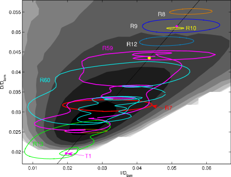
Figure 17: The normalised dissipation $D(t)/D_{lam}$ verses $I/D_{lam}$ for the recurrent flows found at $Re=80$ with the pdf of the DNS turbulence plotted in the background (11 shades at levels $10^{\alpha}$ where $\alpha={-5,-4.5,\ldots,-0.5,0}$). Plotted are $T1$ ($D/D_{lam}=I/D_{lam}=0.0196$), $T3$ (0.0514), $T5$ (0.0435, yellow dot), $R7-R13$ and $R59-R60$.

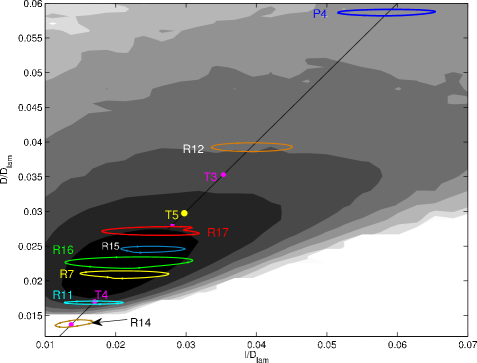
Figure 18: The normalised dissipation $D(t)/D_{lam}$ verses $I/D_{lam}$ for the recurrent flows found at $Re=100$ with the pdf of the DNS turbulence plotted in the background (11 shades at levels $10^{\alpha}$ where $\alpha={-5,-4.5,\ldots,-0.5,0}$). Plotted are $T1$ ($D/D_{lam}=I/D_{lam}=0.0137$), $T3$ (0.0353), $T4$ (0.0170), $T5$ (0.0297, yellow dot), $P4$, $R7$, $R11$, $R12$, $R14-R17$ and $R61$.

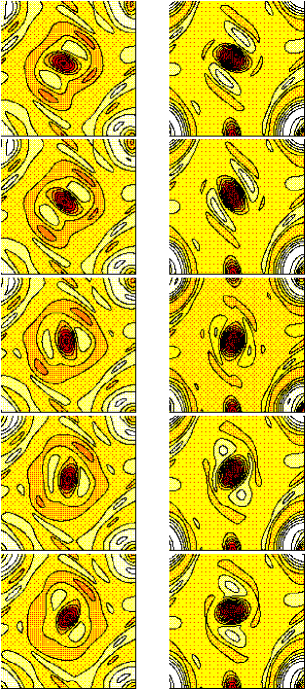
Figure 19: (Low resolution version for the arXiv) The dns trajectory (left) synchronised with the subsequently converged periodic orbit $P4$ (right) at $Re=100$. Time proceeds downwards with snapshots at $t_{0},t_{0}+0.2,t_{0}+0.6,t_{0}+0.8$ and $t_{0}+1.0$ (the period of $P4$ is 1.185). The vorticity scale ranges from -26 (dark red) to 12 (light white).

5 Recurrent flows as a turbulent alphabet

Given the sets of recurrent flows extracted at each $Re$, the question is then how to use them to predict properties of the turbulence encountered. Periodic Orbit Theory advocates a weighted expansion of the recurrent flows such that

$$\Gamma_{prediction}^{N}:=\frac{\sum_{i=1}^{N}w_{i}\Gamma_{i}}{\sum_{i=1}^{N}w_{i}}$$ (40)

where $\Gamma$ is any property such the mean dissipation rate, the mean profile or a pdf, $N$ the total number of recurrent flows and the weights are

$$w_{i}=\left[\prod_{\lambda^{(i)}_{k}\neq 0}|\,(1-e^{\lambda^{(i)}_{k}T^{(i)}})|\,\right]^{-1}$$ (41)

(e.g. Cvitanovic 1995, Lan 2010). Here $\lambda^{(i)}_{k}$ is the $k$th eigenvalue of the linearised operator around the $i$th recurrent flow of period $T^{(i)}$ (the associated Floquet multiplier would be $\mu^{(i)}_{k}:=e^{\lambda^{(i)}_{k}T^{(i)}}$). Calculating the weights in (41) represents a considerable challenge in such a high-dimensional system. Moreover, as already indicated, this expression is derived under special conditions not satisfied by the Navier-Stokes equations (e.g. hyperbolicity) as well as being derived only for (unstable) periodic orbits rather than (unstable) relative periodic orbits (the latter do not exist in very low dimensional systems). A modified theory is being developed (Cvitanovic 2012) to include them but here, in the spirit of what follows, we brush over this subtlety to treat relative periodic orbits just like periodic orbits (see also Lopez et al. 2005). Given these issues, we proceed in a more pragmatic fashion in keeping with the previous suggestive work of Zoldi & Greenside (1998) and Kazantsev (1998,2001) (see also Dettmann & Morriss 1997). These authors proposed and tested a strategy of developing weights based upon only the unstable eigenvalues associated with the recurrent flow (i.e. $\Re e(\lambda_{k}^{(i)})>0$). In particular, Zoldi & Greenside (1998) advocated the ‘escape-time’ weighting

$$w_{i}\propto\frac{1}{\sum_{k\in{\cal K}^{(i)}}Re(\lambda_{k}^{(i)})}\qquad{\rm protocol\,1}$$ (42)

where ${\cal K}^{(i)}$ is the set of $k$ such that $\Re e(\lambda_{k}^{(i)})>0$ since this efficiently captures how unstable the recurrent flow is and inversely correlates this with how long the turbulent trajectory should spend in its vicinity. Kazantsev (1998, 2001) argued that this formula should be modified to reflect the fact that longer period orbits have a greater ‘presence’ in phase space than shorter period orbits and added the period $T^{(i)}$ to the numerator

$$w_{i}\propto\frac{T^{(i)}}{\sum_{k\in{\cal K}^{(i)}}Re(\lambda_{k}^{(i)})}\qquad{\rm protocol\,2}$$ (43)

Significantly, this protocol suppresses any contribution from equilibria or travelling waves. We now test both of these protocols together with a ‘control’ choice of ‘no weighting’ so just

$$w_{i}\propto 1\qquad{\rm protocol\,3}.$$ (44)

The key measures we use to characterise the 2D turbulence simulated here are pdfs of $E(t)$ and $D(t)$ together with the profiles $\bar{u}(y)$, $u_{rms}(y)$ and $v_{rms}(y)$ (the pdf of $I(t)$ was also considered but adds little information to that provided by the pdf for $D(t)$).

5.1 $Re=40$

The pdfs of $E(t)/E_{lam}$ and $D(t)/D_{lam}$ at $Re=40$ are shown in figure 20 along with the predictions using protocols 1-3, that is, the individual pdfs of each recurrent flow are weighted together appropriately to produce an overall pdf as in (40). In the case of $E(t)/E_{lam}$ all three predictions are very good at the central peak of the pdf but each fails to capture the clear shoulder at higher energies in the DNS albeit at a level of the pdf a factor of $\approx 30$ lower. There is a similar story for the $D(t)/D_{lam}$ pdf although in this case, the performance of the stability-motivated protocols 1 and 2 seem noticeably more effective in capturing the DNS pdf. Again, the extremes of the DNS pdf are not captured reflecting the fact, as commented earlier, that perhaps not enough recurrent flows with large or small dissipation excursions have been found. Given the reduced value of the pdf there, these are infrequently visited and thus require very long runs to realistically have a chance to extract them. As already mentioned, what initially looked like long runs of $10^{5}$ time units were actually not long enough. As further independent evidence of this, plots of the mean profiles $\bar{u}(y)$ from each ‘long’ run at the same $Re$ (see Table 1) showed noticeable differences between each other and to the expected asymptotic state which respects all the symmetries of the system. In particular, the obvious symmetry that the mean profile should be invariant under $\pi/2$ shifts in $y$ was clearly violated. To ameliorate this, we decided to ‘symmetrise’ the DNS mean profile by extracting that part ($U^{SR}(y)$) from the signal ($\bar{u}$) which does satisfy all the symmetries listed in §2.1. Explicitly

$$U^{SR}(y):=\frac{1}{2n}\sum^{2n-1}_{m=0}{\cal S}^{-m}U^{R}({\cal S}^{m}y)\qquad{\rm with}\quad U^{R}:=\frac{1}{2}[\,\bar{u}(y)+{\cal R}^{-1}\bar{u}({\cal R}y)\,]$$ (45)

(recall $n=4$) and similarly for $u^{SR}_{rms}$ and $v^{SR}_{rms}$. This process picks out the following Fourier coefficients

$$U^{SR}(y):=\sum_{m=0}a_{m}\sin(4(2m+1)y)\qquad(\,u^{SR}_{rms},v^{SR}_{rms}\,)=\sum_{m=0}(\,b_{m},c_{m}\,)\cos(8my).$$ (46)

from the complete Fourier series for $\bar{u}$, $u_{rms}$ and $v_{rms}$. In particular, the symmetrised mean profile $U^{SR}(y)$ has the leading Fourier modal form of $\sin 4y$, which mimicks the forcing, and a leading correction of $\sin 12y$. Such a profile needs only be plotted over $y\in[0,\pi/4]$ which is done in figure 21 along with the predictions from protocols 1-3. This comparison looks impressive with $a_{0}=0.232$ (cf expression (46)) in the DNS, compared to $0.214$ (protocol 1), $0.215$ (2) and $0.219$ (3). For all, $a_{1}=O(10^{-6})$ and $a_{2}=O(10^{-8})$ (as way of comparison, the ‘raw’ mean flow $\bar{u}$ has a leading non-symmetrised part given by $0.0280\cos y+0.0268\sin y$, i.e. roughly 10% smaller than the symmetrised part). The explanation for why the (symmetrised) mean profile matches the forcing profile so well is currently unclear to us and it is tempting to speculate that actually $a_{n}\rightarrow 0$ ($n\geq 1$) with the period of averaging. Sarris et al. (2007) study the statistics of 3D Kolmogorov flow for various computational domains and use two measures to signal whether their statistics have converged sufficiently over a period of time integration. One,

$$\gamma_{2}:=\frac{(\langle I\rangle_{t}-\langle D\rangle_{t})^{2}}{\langle D\rangle_{t}^{2}}$$ (47)

(equation (22), Sarris et al. 2007) assesses the extent to which the energy input into the flow matches the the energy dissipated and is easily calculated from our output data: $\gamma_{2}$ is at most $O(10^{-8})$ for all our $10^{5}$ time unit runs. Even with this small value, we find evidence that the mean profile is far from converged to what is expected (i.e. satisfies all the symmetries of the problem) which emphasizes how easy it is to unwittingly collect unconverged statistics.

Figure 21 also shows the equivalent plot for $u_{rms}$ and $v_{rms}$. For $u_{rms}$, $b_{0}=0.687$ for the DNS which clearly differs from all the predictions - $0.272$ (protocol 1), $0.289$ (2) and $0.276$ (3). The comparison for $v_{rms}$, however, is much better: $c_{0}=0.933$ for the DNS verses $0.887$ (protocol 1), $0.891$ (2) and $0.879$ (3). One possible reason why the $u_{rms}$ comparison is poor is that $u_{rms}$ is calculated in the DNS ‘on the fly’ by subtracting the current best estimate of the mean $\bar{u}$ from the current streamwise velocity (see 12) rather than using the final mean profile to a posteriori calculate the streamwise fluctuation field. Given our realisation now that the mean profile takes a long time to converge to its (symmetric) asymptotic state, there is likely to be a significant error (henceforth we consider only $v_{rms}$ for $Re=60,80$ and $100$).

An inescapable conclusion from these comparisons so far is that the ‘control’ protocol 3 of actually ‘no weighting’ performs almost as well as the other stability-motivated protocols 1 and 2. It’s worthwhile at this point to clarify why. The upper plot in figure 22 shows how the peak symmetrised mean value, $U^{SR}(\pi/8)$, varies for each recurrent flow and compares these values with the DNS and predictions from the 3 protocols. From this it is clear that most of the recurrent flows are good predictors individually and so when they are mixed together the result is still reasonably good. The lower plot in figure 22 shows how the weights vary across the recurrent flows in the 3 different protocols. Again, there is not that much variation over the majority (although notice that $w_{i}=0$ for $i=1,2,3$ in protocol 2 since $T^{(i)}=0$) which presumably reflects the fact that the stability characteristics of the recurrent flows are all pretty similar.

Figure 20: The probability density functions for $E(t)/E_{lam}$ and $D(t)/D_{lam}$ from DNS (blue thick line) and predictions using weighting protocol 1 (red, thick line with dots), 2 (green, thin line) and 3 (black thick dashed) at $Re=40$. 40 bins were used to calculate the pdfs for the recurrent flows and 100 bins for the DNS due to its greater range. These choices gave the best balance of resolution with the data available.

Figure 21: The symmetrised mean flow $U^{SR}(y)$ (left) and symmetrised $u^{RS}_{rms}(y)$ (right plot left part) and $v^{RS}_{rms}(y)$ (right part of right plot) from DNS (blue thick line) and predictions using weighting protocol 1 (red, thick line with dots), 2 (green, thin line) and 3 (black thick dashed) at $Re=40$.

Figure 22: Top: The peak symmetrised mean $U^{RS}(\pi/8)$ for the DNS (thick blue horizontal line), prediction using protocol 1 (red dotted line), prediction using protocol 2 (green line), the control prediction (dashed black line) and for each recurrent flow listed in the order given in Table 1 at $Re=40$ (so $i=20$ is $R25$ and $i=45$ is $R50$ marked with black dotted lines). Bottom: the weights for the three protocols (1-red line with dots, 2-green line, 3-black horizontal line) plotted for all the recurrent structures at $Re=40$. Again the vertical (black) dotted lines indicate $R25$ and $R50$.

5.2 $Re=60,80$ & $100$

The smaller number of recurrent flows extracted for $Re>40$ means that it is harder to generate reasonably smooth predictions for the pdfs of the energy and dissipation. While the same number of 100 bins as at $Re=40$ can be used to generate a smooth DNS pdf, only 60 bins could be used to sum the pdfs of the recurrent flows. This number produced the best compromise of granularity across the range while ensuring that there is enough data in each bin for (reasonable) smoothness at least for $Re=60$ and $Re=80$ (the sparse coverage of the dissipation range by the recurrent flows at $Re=100$ - see figure 18 - prevented any useful plot to be generated). Figure 23 shows the result of this procedure for the dissipation pdf at $Re=60$ and $80$ (plots not shown for the energy are similar). Here, protocol 2 offers the best partial fit both at $Re=60$ and $Re=80$ although it is clear that much of the turbulent dissipation range extends higher than any of the recurrent flows found at both $Re$ (also clear from 16 and 17) and that the ‘prediction’ is of limited quality. It’s also worth remarking that the predictions are now more distinquishable at these higher $Re$ which can be traced back to the separating stability characteristics of the recurrent flows. For example, $E1$ has $\sum\Re e(\lambda_{j})=5.053$ whereas this is just $0.139$ for $T1$.

Figure 24 shows the symmetrised mean profile as calculated from the DNS and predicted by the 3 protocols at $Re=60$ and $Re=80$. Again, somewhat paradoxically, the ‘control’ protocol does the best job in both cases. At $Re=60$ $a_{0}=0.2277$, $0.2298$ and $0.2296$ (cf expression (46)) across the three series A DNS runs listed in Table 1 (with again $\approx 10\%$ non-symmetrised part in all cases). In comparison, $a_{0}=0.148$ (protocol 1), $0.175$ (2) and $0.200$ (3). For $v_{rms}$, $c_{0}=1.099$ in the DNS run to be compared with the predictions of $1.064$ (protocol 1), $1.057$ (2) and $1.055$ (3). At $Re=80$, $a_{0}=0.2009$, $0.2016$ and $0.1998$ across the three series A DNS runs listed in Table 1. In comparison, $a_{0}=0.1416$ (protocol 1), $0.1403$ (2) and $0.1944$ (3).

Finally, we note that at $Re=100$, $a_{0}=0.1777$, $0.1782$ and $0.1783$ across the three series A DNS runs listed in Table 1 (with now $\approx 20\%$ non-symmetrised part in all cases).

Figure 23: The probability density functions for $D(t)/D_{lam}$ from DNS (blue thick line, cyan and magenta lines) and predictions using weighting protocol 1 (red, thick line with dots), 2 (green, thin line with triangles), and 3 (black thick dashed with squares) at $Re=60$ (left) and $Re=80$ (right). 60 bins were used to calculate the pdfs for the recurrent flows and 100 bins for the DNS due to its greater range. These choices gave the best balance of resolution with the data available.

Figure 24: The symmetrised mean flow $U^{SR}(y)$ from DNS (blue thick line) and predictions using weighting protocol 1 (red, thick line with dots), 2 (green, thin line) and 3 (black thick dashed) for $Re=60$ (left) and $Re=80$ (right).

6 Discussion

In this study, we have considered 2D turbulence on the torus $[0,2\pi]^{2}$ forced monochromatically in one direction (Kolmogorov flow). By looking for near recurrences of the flow in long direct numerical simulation runs, sets of exactly closed flow solutions ‘embedded’ in this turbulence have been extracted at different forcing amplitudes ($Re$). We have then tried to use these sets of recurrent flows to reconstruct key statistics of the turbulence motivated by Periodic Orbit Theory in low-dimensional chaos. The approach has been reasonably successful at $Re=40$ - see figures 20 and 21 - where 50 recurrent flows were found with the majority buried in the part of phase space most populated by the turbulence. In contrast, at $Re=60$, $80$ and $100$, the limited size of the recurrent flow sets found has made the approach largely impotent. Even at $Re=40$, the success achieved seems more reliant on just extracting lots of similar-looking recurrent flows buried in the most popular part of phase space for the turbulence than on any sophisticated choice of weighting coefficients. Indeed, one is reminded of Kawahara & Kida’s (2001) conclusion that one judiciously chosen periodic orbit is ‘enough’ to be a valuable proxy of the turbulence. We can sympathise with this viewpoint but only if the comparison with the turbulence statistics is not too demanding. The key issue, of course, plaguing this investigation is the paucity of recurrent flows found from the finite DNS data generated. This is perhaps the main message to come out of this work: Periodic Orbit theory for fluid turbulence is a promising approach but only if enough - O(100)? - recurrent flows are gathered which requires very long turbulence data sequences. A time sequence of $10^{5}$ time units seems marginally adequate for $Re=40$ but is maybe two orders of magnitude too short for $Re=60$ and beyond. Unfortunately, without these large sets, it has been impossible to discern between different weighting protocols.

Operationally, the work described here has been time-consuming both computationally in generating near-recurrence episodes and attempting to converge them, as well as ‘manually’ because of all the careful processing (e.g. calculating their stability) and archiving of the recurrent flows needed (e.g. does a new convergence from a DNS guess represent a new recurrent flow or a repeat of a previously extracted flow?). Fortunately, there is no reason why this process could not be automated with the objective being to ‘automatically’ generate a basis set of recurrent flows for each $Re$. Indeed, one could hope that such a set at given $Re=Re_{1}$ could be used to predict the turbulent statistics at another $Re=Re_{2}$. This would require each recurrent flow at $Re_{1}$ being continued to $Re_{2}$ and the fresh weights for an expansion being generated from the (new) stability information for each recurrent flow - again painstaking work but readily automated. One fly in the ointment is the possibility of bifurcations in the interval $[Re_{1},Re_{2}]$, particularly saddle node bifurcations where two recurrent flows at $Re_{1}$ merge and annihilate before $Re$ reaches $Re_{2}$. Working with large enough recurrent flow sets would presumably smooth over this effect somewhat but will not eliminate it entirely.

Leaving aside these issues for a moment, it’s worth re-emphasizing that any recurrent flow extracted from DNS data is a simple invariant solution ‘buried’ in the turbulence. As such, each represents a sustained sequence of dynamical processes which contributes to, if not underpins, the turbulence itself. Since they are closed in time, they can be analysed relatively easily in whatever detail is required to understand key dynamical relationships in the flow. This seems a very promising byproduct of the analysis whether one believes a Periodic Theory-type expansion of turbulence is possible or not (pursuing this has not been the focus here due to the 2-dimensionality of the flow).

Finally, the ever-improving computational resources available now have only recently made this type of study possible. Even with these, we have underestimated the demands of data collection in 2D turbulence over the small torus $[0,2\pi]^{2}$. Major challenges ahead include treating large aspect ratio domains - can we find localised recurrent flows? - and handling fully 3 dimensional flows - with automated machinery, will the approach be practical? There is plenty to explore.

Acknowledgements: We both would like to thank Peter Bartello for generously sharing his DNS code. GJC would like to thank Iain Waugh for guidance on arc-length continuation and RRK is grateful to Predrag Cvitanovic for always being willing to talk.

Appendix A

The Newton-GMRES-Hook-step algorithm described in the main text is easily extended to continue solutions over parameter space such as $Re$ or the domain geometry (e.g. $\alpha$). We briefly describe this extension for solution branch continuation in $Re$ which was used to generate figure 14. A simple strategy is to use the solution ${\bf x}(Re)$ as an initial guess in the Newton-GMRES-Hook-step algorithm with the hope of converging to ${\bf x}(Re+\delta Re)$. This should work provided that $\delta Re$ is ‘small enough’ but is ill-equipped to negotiate turning points in the solution branch. A standard, more sophisticated approach is arc-length continuation which uses the branch arc-length as a natural, monotonically-increasing, parametrisation of the solution branch. The key idea is to take small controllable steps in the arc-length rather than $Re$. As a result the state vector needs to be extended as follows

$$\mbox{\boldmath$x$}=\left[\begin{array}[]{c}{\bf\Omega}\\ s\\ T\\ Re\end{array}\right]$$ (48)

and an extra equation

$$\frac{\partial{\bf x}}{\partial r}\cdot\frac{\partial{\bf x}}{\partial r}=1$$ (49)

added to determine $Re$. Previous converged solutions $\mbox{\boldmath$x$}(r_{-1})$ and $\mbox{\boldmath$x$}(r_{0})$ indicate a reasonable step size in $r$, $\delta r=r_{0}-r_{-1}=\sqrt{(\mbox{\boldmath$x$}(r_{0})-\mbox{\boldmath$x$}(r_{-1}))^{2}}$ and allow a prediction to be made for the next solution

$$\mbox{\boldmath$x$}(r_{1})\approx\mbox{\boldmath$x$}(r_{0})+\delta r\frac{\partial\mbox{\boldmath$x$}}{\partial r}\biggl{|}_{r_{0}}\biggr{.}$$ (50)

Given $\mbox{\boldmath$x$}(r_{0})$ and $\delta r$, the extra constraint for the Newton method comes from approximating (49) as follows

$${\cal N}(\mbox{\boldmath$x$}^{n}):=\frac{\partial\mbox{\boldmath$x$}}{\partial r}\biggl{|}_{r_{0}}\biggr{.}(\mbox{\boldmath$x$}^{n}-\mbox{\boldmath$x$}(r_{0}))-\delta r\approx 0$$ (51)

for the $n$th iterate to estimate $\mbox{\boldmath$x$}(r_{1})$. Writing $\delta\mbox{\boldmath$x$}^{n}:=\mbox{\boldmath$x$}^{n+1}-\mbox{\boldmath$x$}^{n}$, then setting

$${\cal N}(\mbox{\boldmath$x$}^{n+1})=\delta x^{n}.\frac{\partial\mbox{\boldmath$x$}}{\partial r}\left|{}_{r_{0}}\right.+{\cal N}(\mbox{\boldmath$x$}^{n})=0$$ (52)

puts the required extra constraint on the iterative improvement $\delta\mbox{\boldmath$x$}^{n}$. The Newton problem (28) then becomes

$$\left[\begin{array}[]{c|c|c|c}\ddots&\vspace{0.0cm}\vdots&\vspace{0.0cm}\vdots&\vdots\\ \hskip 28.45274pt{\displaystyle\frac{\partial{\bf\hat{\Omega}_{s}}}{\partial{\bf\Omega}_{0}}}-{\bf I}&\mathsfi{T}_{x}{\bf\hat{\Omega}_{s}}&{\displaystyle\frac{\partial{\bf\hat{\Omega}_{s}}}{\partial T}}&{\displaystyle\frac{\partial{\bf\hat{\Omega}_{s}}}{\partial Re}}\\ \hskip 56.9055pt\ddots&\vdots&\vdots&\vdots\\ \hline\cr\cdots\quad(\mathsfi{T}_{x}{\bf\Omega}_{0})^{T}\quad\cdots&0&0&0\\ \hline\cr\cdots\quad{\displaystyle\frac{\partial{\bf\Omega}_{0}}{\partial t}^{T}}\quad\cdots&0&0&0\\ \hline\cr\lx@intercol\hfil\cdots\quad{\displaystyle\frac{\partial\mbox{\boldmath$x$}_{0}}{\partial r}^{T}}\quad\cdots\hfil\lx@intercol\\ \end{array}\right]\left[\begin{array}[]{c}\vdots\\ \\ \vspace{0.25cm}\delta{\bf\Omega}\\ \vdots\\ \\ \delta s\\ \\ \\ \delta T\\ \\ \\ \delta Re\\ \end{array}\right]=-\left[\begin{array}[]{c}\vdots\\ \\ \vspace{0.25cm}{\bf F}({\bf\Omega}_{0},s_{0},T_{0};m)\\ \vdots\\ \\ 0\\ \\ \\ 0\\ \\ \\ {\cal N}(\mbox{\boldmath$x$}_{0})\\ \end{array}\right]$$ (53)

Depending on how easily convergence is obtained, $\delta r$ can be increased or decreased if the algorithm shows signs of divergence. A second order approach to estimating $\partial\mbox{\boldmath$x$}/\partial r$ was actually adopted for the predictive step but the first order estimate proved sufficient for the constraint present in (53).

References

- [Armbruster (1996))] Armbruster, D., Nicolaenko, B., Smaoui, N. & Chossat, P. 1996 Symmetries and dynamics of 2-D Navier-Stokes flow Physica D 95, 81-93.
- [Arnold (1960))] Arnol’d, V.I., Meshalkin, L.D. 1960 The seminar of A.N. Kolmogorov on selected topics in analysis (1958-1959) Uspekhi Mat. Nauk 15, 247-250.
- [Auerbach et al. (1987)] Auerbach, D., Cvitanovic, P. Eckmann, J.-P., Gunaratne, G. and Procaccia, I. 1987 Exploring chaotic motion through periodic orbits Phys. Rev. Lett. 58, 2387-2389.
- [Artuso et al. (1990a)] Artuso, R. Aurell, E., Cvitanovic, P. 1990a Recycling of strange sets: I Cycle expansions. Nonlinearity 3, 325-359.
- [Artuso et al. (1990b)] Artuso, R. Aurell, E., Cvitanovic, P. 1990b Recycling of strange sets: II Applications. Nonlinearity 3, 361-386.
- [Bartello Warn (1996)] Bartello, P. and Warn, T. 1996 Self-similarity of decaying two-dimensional turbulence J. Fluid Mech. 326, 357-372.
- [Boffetta Musacchio (2010)] Boffetta, G. and Musacchio, S. 2010 Evidence for a double cascade scenario in two-dimensional turbulence Phys. Rev. E. 82, 016307.
- [Boghosian et al. (2011)] Boghosian, B.M., Fazendeiro, L.M., Lätt, J., Tang, H. & Coveney, P.V. 2011 New variational principles for locating periodic orbits of differential equations Phil. Trans. R. Soc. A 369, 2211-2218.
- [Bondarenko (1979))] Bondarenko, N.F., Gak, M.Z. & Dolzhanskii, F.V. 1979 Laboratory and theoretical models of plane periodic flow Izv. Acad. Sci. USSR Atmospher. Ocean. Phys. 15, 711-716.
- [Borue] Borue, V. & Orszag, S.A. 1996 Numerical study of three-dimensional Kolmogorov flow at high Reynolds numbers J. Fluid Mech. 306, 293-323.
- [Burgess et al. 1999] Burgess, J.M., Bizon, C., McCormick, W.D., Swift, J.B. & Swinney, H.L. 1999 Instability of the Kolmogorov flow in a soap film Phys. Rev. E 60, 715-721.
- [Christiansen et al. (1997)] Christiansen, F., Cvitanovic, P. & Putkaradze, V. 1997 Spatiotemporal chaos in terms of unstable recurrent patterns Nonlinearity 10, 55-70.
- [Cvitanovic (1988)] Cvitanovic, P. 1988 Invariant measurement of strange sets in terms of cycles Phys. Rev. Lett. 61, 2729-2732.
- [Cvitanovic (1992)] Cvitanovic, P. 1992 Periodic orbit theory in classical and quantum mechanics Chaos 2, 1.
- [Cvitanovic et al (2005)] Cvitanovic, P., Artuso, R., Dahlqvist, P. Mainieri, R., Tanner, G., Vattay, G., Whelan, N. and Wirzba, A. 2005 Classical and Quantum Chaos webbokk available at http://chaosbook.org
- [Cvitanovic (2010))] Cvitanovic, P. & Gibson, J.F. 2010 Geometry of turbulence in wall-bounded shear flows: periodic orbits Physica Scripta 142, 014007.
- [Cvitanovic et al (2010)] Cvitanovic, P., Davidchack, R. & Evangelos, S. 2010 On the state space geometry of the Kuramoto-Sivashinsky flow in a periodic domain SIAM J. Appl. Dyn. Sys. 9, 1-33.
- [Cvitanovic (2012)] Cvitanovic, P. 2012 Continuous symmetry reduced trace formulas preprint .
- [Dennis Schnabel (1996))] Dennis, J.E. & Schnabel, R.B. Numerical Methods for Unconstrained Optimisation and Nonlinear equations SIAM Classics (SIAM, Philadelphia, 1996).
- [Dettmann Morriss (1997)] Dettmann, C.P. & Morriss, G.P. 1997 Stability ordering of cycle expansions Phys. Rev. Lett. 78, 4201-4204.
- [Duguet et al (2008)] Duguet, Y., Pringle, C.C.T. & Kerswell, R.R. 2008 Relative periodic orbits in transitional pipe flow Phys. Fluids 20, 114102.
- [Eckhardt et al. (2002)] Eckhardt, B., Faisst, H., Schmiegel, A. & Schumacher, J. 2002 Turbulence transition in shear flows Advances in Turbulence IX: Proc. 9th European Turbulence Conf. (Southampton) ed. I.P. Castro et al. (Barcelona: CISME) p 701
- [Eckhardt et al. (2007)] Eckhardt, B., Schneider, T.M., Hof, B. & Westerweel, J. 2007 Turbulence transition in pipe flow Ann. Rev. Fluid Mech. 39, 447-468.
- [Eckmann & Ruelle (1985)] Eckmann, P. & Ruelle, D. 1985 Ergodic theory of chaotic systems Reviews of Modern Physics 57, 617-656.
- [Fazendeiro et al. (2010] Fazendeiro, L., Boghosian, B.M., Coveney, P.V. & Lätt, J. 2010 Unstable periodic orbits in weak turbulence J. Comput. Sci. 1, 13-23.
- [Gibson et al (2008))] Gibson, J.F., Halcrow, J. & Cvitanovic, P. 2008 Visualizing the geometry of state space in plane Couette flow J. Fluid Mech. 611, 107-130.
- [Gibson et al (2009))] Gibson, J.F., Halcrow, J. & Cvitanovic, P. 2009 Equilibrium and travelling-wave solutions of plane Couette flow J. Fluid Mech. 638, 243-266.
- [Gotoh)] Gotoh, K. & Yamada, M. 1986 The instability of rhombic cell flows Fluid Dyn. Res. 1, 165-176.
- [Halcrow et al. 2009)] Halcrow, J., Gibson, J.F., Cvitanovic, P. & Viswanath, D. 2009 Heteroclinic connections in plane Couette flow J. Fluid Mech. 621, 365-376
- [Hamilton et al. 1995] Hamilton, J.M., Kim, J. & Waleffe, F. 1995 Regeneration mechanism of near-wall turbulence structures J. Fluid Mech. 287, 317-348.
- [Hof et al (2004))] Hof, B., van Doorne, C.W.H., Westerweel, J., Nieuwstadt, F.T.M., Faisst, H., Eckhardt, B., Wedin, H., Kerswell, R.R. & Waleffe F. 2004 Experimental observation of nonlinear traveling waves in turbulent pipe flow. Science 305, 1594-1598.
- [Holmes, Lumley & Berkooz (1996)] Holmes, P., Lumley, J.L. & Berkooz, G. 1996 Turbulence, Coherent Structures, Dynamical Systems and Symmetry (Cambridge, Cambridge University Press)
- [Hopf (1948)] Hopf, E. 1948 A mathematical example displaying features of turbulence Commun. Appl. Math. 1, 303-322
- [Kawahara Kida (2001] Kawahara, G. & Kida, S. 2001 Periodic motion embedded in plane Couette turbulence: regenerative cycle and burst J. Fluid Mech. 449, 291-300.
- [Kawahara et al (2012] Kawahara, G. Uhlmann, M. & van Veen, L. 2012 The significance of simple invariant solutions in turbulent flows Ann. Rev. Fluid Mech. 44, 203-225.
- [Kazantsev (1998)] Kazantsev, E. 1998 Unstable periodic orbits and attractor of the barotropic ocean model Nonlin. Proc. Geophys. 5, 193-208.
- [Kazantsev (2001)] Kazantsev, E. 2001 Sensitivity of the attractor of the barotropic ocean model to external influences: approach by unstable periodic orbits Nonlin. Proc. Geophys. 8, 281-300.
- [Kerswell (2005)] Kerswell, R.R. 2005 Recent Progress in understanding the transition to turbulence in a pipe Nonlinearity 18, R17-R44.
- [Kim)] Kim, S-C. & Okamoto, H. 2003 Bifurcations and inviscid limit of rhombic Navier-Stokes flows in tori IMA J. Appl. Math. 68, 119-134.
- [Lan (2010)] Lan, Y. 2010 Cycle expansions: From maps to turbulence Commun. Nonlinear Sci. Numer. Simulat. 15, 502-526.
- [Lan Cvitanovic (2004)] Lan, Y. & Cvitanovic, P. 2004 Variational method for finding periodic orbits in a general flow Phys. Rev. E. 69, 016217.
- [Lan Cvitanovic (2008)] Lan, Y. & Cvitanovic, P. 2008 Unstable recurrent patterns in Kuramoto-Sivashinsky dynamics Phys. Rev. E 78, 026208.
- [Lopez et al (2005)] Lopez, V., Boyland, P., Heath, M.T. and Moser, R.D. 2005 Relative periodic solutions of the complex Ginzburg-Landau equation SIAM J. App. Dyn. Sys. 4, 1042-1075.
- [MacKay & Miess (1987)] MacKay, R.S. & Miess, J.D. 1987 Hamiltonian Dynamical Systems (Adam Hilger, Bristol)
- [Marchioro (1986))] Marchioro, C. 1986 An example of absence of turbulence for any Reynolds number Commun. Math. Phys. 105, 99-106.
- [Meshalkin (1961))] Meshalkin, L.D. & Sinai, Ya. G. 1961 Investigation of stability of a steady-state solution of a system of equations for the plane motion of an incompressible viscous liquid Prik. Mat. Mech. 25, 1140-1143.
- [Obukhov(1983))] Obukhov, A.M. 1983 Kolmogorov flow and laboratoty simulation of it Uspekhi Mat. Nauk 38, 101-111.
- [Okamato Shoji 1993] Okamoto, H. & Shoji, M. 1993 Bifurcation diagrams in Kolmogorov’s problem of viscous incompressible fluid on 2-D flat tori Japan J. Indust. Appl. Math. 10, 191-218.
- [Panton (1997))] Panton, R.L. 1997 ed. Self-Sustaining Mechanisms of Wall Turbulence. (Southampton: Computational Mechanics Publications)
- [Platt et al. (1991)] Platt, N., Sirovich, L. & Fitzmaurice, N. 1991 An investigation of chaotic Kolmogorov flows Phys. Fluids 3, 681–696.
- [Poincaré (1892)] Poincaré, H. 1892 Les méthodes nouvelles de la méchanique céleste (Guthier-Villars, Paris)
- [Robinson (1991))] Robinson, S.K. 1991 Coherent motions in the turbulent boundary layer Ann. Rev. Fluid Mech. 23, 601-639.
- [Ruelle (1978)] Ruelle, D. 1978 Statistical Mechanics, Thermodynamic Formalism (Addison-Wesley, Reading, MA)
- [Saad (1986)] Saad, Y. & Schultz, M.H. 1986 GMRES: A generalized minimal residual algorithm for solving nonsymmetric linear systems SIAM J. Sci. Stat. Comput. 7, 856–869.
- [Sarris et al (2007)] Sarris, I.E., Jeanmart, H., Carati, D. and Winckelmans, G. 2007 Box-size dependence and breaking of translational invariance in the velocity statistics computed from three-dimensional turbulent Kolmogorov flows Phys. Fluids 19, 095101.
- [She (1988)] She, Z.S. 1988 Large-scale dynamics and transition to turbulence in the two-dimensional Kolmogorov flow Proceedings on Current Trends in Turbulence Research eds. H. Branover, M. Mond & Y. Unger (American Institute of Aeronautics and Astronautics, Washington, D.C.) 117, 374-396.
- [Shebalin)] Shebalin, J.V. & Woodruff, S.L. 1997 Kolmogorov flow in three dimensions Phys. Fluids 9, 164-170.
- [Sommeria (1986))] Sommeria, J. 1986 Experimental study of the two-dimensional inverse energy cascade in a square box J. Fluid Mech. 170, 139-168.
- [Trefethen (1997)] Trefethen, L.N. & Bau D. 1997 Numerical Linear Algebra SIAM, ISBN 978-0-89871-361-9.
- [Tsang Young 2008] Tsang, Y-K. & Young, W.R. 2008 Energy-enstrophy stability of beta-plane Kolmogorov flow with drag Phys. Fluids 20, 084102.
- [van Veen et al (2006)] van Veen, L. Kawahara, G. & Kida, S. 2006 Periodic motion representing isotropic turbulence Fluid Dyn. Res. 38, 19-46.
- [Viswanath (2007)] Viswanath, D. 2007 Recurrent motions within plane Couette turbulence J. Fluid Mech. 580, 339-358.
- [Viswanath (2009)] Viswanath, D. 2009 The critical layer in pipe flow at high Reynolds number Phil. Trans R. Soc. A 367, 561–576.
- [Waleffe (1997)] Waleffe, F. 1997 On a self-sustaining process in shear flows Phys. Fluids 9, 884-900.
- [Zoldi & Greenside 1998)] Zoldi, S. & Greenside, H.S. 1998 Spatially localised unstable periodic orbits of a high-dimensional chaotic system Phys. Rev. E 57, R2511.