Sinusoidally-driven unconfined compression test for a biphasic tissue

Abstract

In recent years, a number of experimental studies have been conducted to investigate the mechanical behavior of water-saturated biological tissues like articular cartilage under dynamic loading. For in vivo measurements of tissue viability, the indentation tests with the half-sinusoidal loading history were proposed. In the present paper, the sinusoidally-driven compression test utilizing either the load-controlled or displacement-controlled loading protocol are considered in the framework of linear biphasic layer model. Closed-form analytical solutions for the integral characteristics of the compression test are obtained.

1 Introduction

It is well known that the long-term creep and relaxation tests, typically used for determining viscoelastic and biphasic/poroelastic properties, are not appropriate for rapidly assessing the dynamic biomechanical properties of biological tissues like articular cartilage. For in vivo measurements of tissue viability, Appleyard et al. (2001) developed a dynamic indentation instrument, which employs a single-frequency (20 Hz) sinusoidal oscillatory waveform superimposed on a carrier load. It is to note that the oscillation test requires some time period to elapse before recording the measurement to minimize the influence of the initial conditions. That is why the indentation or compression tests with the half-sinusoidal loading history are so tempting. In particular, the half-sinusoidal history is useful for developing indentation-type scanning probe-based nanodevices reported by Stolz et al. (2007). Also, as a first approximation, such a indentation history can be used for modeling impact tests (Butcher and Segalman, 1984).

In the present paper, it is assumed that the mechanical response of a time-dependent material can be described in the framework of biphasic layer model. Following Argatov (2012), we consider sinusoidally-driven flat-ended compression test utilizing either the load-controlled or displacement-controlled loading protocol. Closed-form analytical solutions for the integral characteristics of the compression test are obtained.

2 Unconfined compression of a cylindrical biphasic sample

We assume that the unconfined compression test for a soft biological tissue sample can be described by a one-dimensional axisymmetric mathematical model of Armstrong et al. (1984) developed in the framework of the linear biphasic theory (Mow et al., 1980). In particular, it is assumed that a thin cylindrical specimen is squeezed between two perfectly smooth, impermeable rigid plates such that compressive strain in the axial direction (see, Fig. 1) is homogeneous.

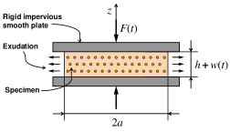
Figure 1: Schematics of the unconfined compression test.

Let $F(t)$ and $w(t)$ denote, respectively, the variable compressive force and the vertical displacement of the upper plate with respect to the lower plate ($t$ is the time variable). Then, the compressive strain is defined as

$$\epsilon(t)=\frac{w(t)}{h},$$ (1)

where $h$ is the sample thickness. (Note that compressive strain is negative.)

Let us also introduce the non-dimensional variables

$$\hat{F}=\frac{F}{\pi a^{2}\mu_{s}},\quad\hat{t}=\frac{H_{A}kt}{a^{2}},$$ (2)

where $H_{A}=\lambda_{s}+2\mu_{s}$, $\mu_{s}$ and $\lambda_{s}$ are the confined compression modulus and Lamé constants of the elastic solid matrix, respectively, $k$ is the tissue permeability, $a$ is the radius of specimen, $\hat{t}$ is the dimensionless time, $\hat{F}$ is the dimensionless force.

Finally, let $\bar{F}(s)$ and $\bar{\epsilon}(s)$ denote the Laplace transforms with respect to the dimensionless time, and $s$ is the Laplace transform parameter. According to Armstrong et al. (1984), the following relationship holds true:

$$\bar{F}(s)=s\bar{\epsilon}(s)\bar{K}(s),$$ (3)

$$\bar{K}(s)=\frac{\displaystyle 3I_{0}(\sqrt{s})-\frac{8\mu_{s}}{H_{A}}\frac{I_{1}(\sqrt{s})}{\sqrt{s}}}{\displaystyle s\Bigl{(}I_{0}(\sqrt{s})-\frac{2\mu_{s}}{H_{A}}\frac{I_{1}(\sqrt{s})}{\sqrt{s}}\Bigr{)}}.$$ (4)

Here, $I_{0}$ and $I_{1}$ are modified Bessel functions of the first kind.

By applying the convolution theorem to Eq. (3), we obtain

$$\hat{F}(\hat{t})=\int\limits_{0-}^{\hat{t}}\frac{d\epsilon(\tau)}{d\tau}\hat{K}(\hat{t}-\tau)\,d\tau,$$ (5)

where $\hat{K}(\hat{t})=\mathcal{L}^{-1}\{\bar{K}(s)\}$ is the original function of $\bar{K}(s)$, $t=0-$ is the time moment just preceding the initial moment of loading. In deriving Eq. (5), we used the formula

$$\mathcal{L}^{-1}\{s\bar{\epsilon}(s)\}=\frac{d\epsilon(\hat{t})}{d\hat{t}}+\epsilon(0+)\delta(\hat{t}),$$

where $\delta(\hat{t})$ is the Dirac function.

By using the results obtained by Armstrong et al. (1984), we will have

$$\hat{K}(\hat{t})=2(1+\nu_{s})+\sum_{n=1}^{\infty}2(1+\nu_{s})A_{n}\exp(-\alpha_{n}^{2}\hat{t}),$$ (6)

$$A_{n}=\frac{(1-\nu_{s})(1-2\nu_{s})}{(1+\nu_{s})[(1-\nu_{s})^{2}\alpha_{n}^{2}-(1-2\nu_{s})]}.$$ (7)

Here, $\alpha_{n}$ are the roots of the characteristic equation (with $J_{0}$ and $J_{1}$ being Bessel functions of the first kind)

$$J_{0}(x)-\frac{(1-2\nu_{s})}{(1-\nu_{s})}\frac{J_{1}(x)}{x}=0.$$

The inverse relation for Eq. (5) can be represented as

$$\epsilon(\hat{t})=\int\limits_{0-}^{\hat{t}}\frac{d\hat{F}(\tau)}{d\tau}\hat{M}(\hat{t}-\tau)\,d\tau,$$ (8)

where $\hat{M}(\hat{t})=\mathcal{L}^{-1}\{\bar{M}(s)\}$ with $\bar{M}(s)$ defined by the formula

$$\bar{M}(s)=\frac{\displaystyle I_{0}(\sqrt{s})-\frac{2\mu_{s}}{H_{A}}\frac{I_{1}(\sqrt{s})}{\sqrt{s}}}{\displaystyle s\Bigl{(}3I_{0}(\sqrt{s})-\frac{8\mu_{s}}{H_{A}}\frac{I_{1}(\sqrt{s})}{\sqrt{s}}\Bigr{)}}.$$ (9)

Again, making use of the results by Armstrong et al. (1984), we get

$$\hat{M}(\hat{t})=\frac{1}{2(1+\nu_{s})}-\sum_{n=1}^{\infty}\frac{B_{n}}{2(1+\nu_{s})}\exp(-\beta_{n}^{2}\hat{t}),$$ (10)

$$B_{n}=\frac{4(1-\nu_{s}^{2})(1-2\nu_{s})}{9(1-\nu_{s})^{2}\beta_{n}^{2}-8(1+\nu_{s})(1-2\nu_{s})},$$ (11)

where $\beta_{n}$ are the roots of the corresponding characteristic equation

$$J_{0}(x)-\frac{4(1-2\nu_{s})}{3(1-\nu_{s})}\frac{J_{1}(x)}{x}=0.$$

The short-time asymptotic approximation for the kernel $\hat{K}(\hat{t})$ (the same can be done with $\hat{M}(\hat{t})$) can be obtained by evaluating the inverse of $\bar{K}(s)$ as $s\to\infty$. For this purpose, we apply the well known asymptotic formula (see, e.g., (Gradshteyn and Ryzhik, 1980))

$$I_{n}(z)=\frac{e^{z}}{\sqrt{2\pi z}}\Bigl{\{}1+\frac{(1-4n^{2})}{8z}+O(z^{-2})\Bigr{\}}.$$ (12)

Making use of (12), we expand the right-hand sides of (4) and (9) in terms of $1/\sqrt{s}$. As a result, we arrive at the following asymptotic expansions (note a misprint in formula (36b) in (Armstrong et al., 1984)):

$$\hat{K}(\hat{t})=3-\frac{2(1-2\nu_{s})}{\sqrt{\pi}(1-\nu_{s})}\sqrt{\hat{t}}+O(\hat{t}),\quad\hat{t}\to 0,$$ (13)

$$\hat{M}(\hat{t})=\frac{1}{3}+\frac{2(1-2\nu_{s})}{9\sqrt{\pi}(1-\nu_{s})}\sqrt{\hat{t}}+O(\hat{t}),\quad\hat{t}\to 0.$$ (14)

The asymptotic approximations (13) and (14) can be used for evaluating impact unconfined compression test with the impact duration relatively small compared to the so-called gel diffusion time for the biphasic material $t_{g}=a^{2}/(H_{A}k)$.

In the dimensional form, Eqs. (5) and (8) can be recast as follows:

$$F(t)=\frac{\pi a^{2}E_{s}}{h}\int\limits_{0-}^{t}\frac{dw(\tau)}{d\tau}K(t-\tau)\,d\tau,$$ (15)

$$w(t)=\frac{h}{\pi a^{2}E_{s}}\int\limits_{0-}^{t}\frac{dF(\tau)}{d\tau}M(t-\tau)\,d\tau.$$ (16)

Here we introduced the notation

$$K(t)=1+\sum_{n=1}^{\infty}A_{n}\exp\Bigl{(}-\frac{t}{\rho_{n}}\Bigr{)},$$ (17)

$$M(t)=1-\sum_{n=1}^{\infty}B_{n}\exp\Bigl{(}-\frac{t}{\tau_{n}}\Bigr{)},$$ (18)

$$\rho_{n}=\frac{a^{2}}{\alpha_{n}^{2}H_{A}k},\quad\tau_{n}=\frac{a^{2}}{\beta_{n}^{2}H_{A}k}.$$ (19)

Note that the sequences $\rho_{1}>\rho_{2}>\ldots$ and $\tau_{1}>\tau_{2}>\ldots$, which are defined by formulas (19), represent the discrete relaxation and retardation spectra, respectively. Recall that the coefficients $A_{n}$ and $B_{n}$ are defined by formulas (7) and (11).

Further, in view of (13) and (14), we will have

$$K_{0}=K(0)=\frac{3}{2(1+\nu_{s})},$$ (20)

$$M_{0}=M(0)=\frac{2}{3}(1+\nu_{s}).$$ (21)

Hence, the following equalities take place:

$$1+\sum_{n=1}^{\infty}A_{n}=\frac{3}{2(1+\nu_{s})},$$ (22)

$$1-\sum_{n=1}^{\infty}B_{n}=\frac{2}{3}(1+\nu_{s}).$$ (23)

Now, using formula (21), we can rewrite the function (18) as

$$M(t)=M_{0}+\sum_{n=1}^{\infty}B_{n}\Bigl{(}1-\exp\Bigl{(}-\frac{t}{\tau_{n}}\Bigr{)}\Bigr{)}.$$ (24)

By analogy with the viscoelastic model, the functions $K(t)$ and $M(t)$ will be called the biphasic relaxation and creep functions for unconfined compression.

3 Cyclic compressive loading

Following Li et al. (1995), we assume that a biphasic tissue sample is subjected to a cyclic displacement input

$$w(t)=[w_{0}(1-\cos\omega t)+w_{1}]H(t),$$ (25)

where $H(t)$ is the Heaviside function, $w_{1}/h$ is the prestrain resulting from the initial deformation applied to the sample to create the desired preload, $w_{0}$ is the displacement amplitude, i.e., $w_{0}/h$ is equal to one-half the peak-to-peak cyclic strain input superimposed on the prestrain, and $\omega=2\pi f$ is the angular frequency with $f$ being the loading frequency.

Differentiating (25), we get

$$\frac{dw(t)}{dt}=H(t)w_{0}\omega\sin\omega t+w_{1}\delta(t).$$ (26)

Now, substituting the expression (26) into Eq. (15), we arrive, after some algebra, at the following resulting stress output:

$$\frac{F(t)}{\pi a^{2}} = \frac{E_{s}}{h}\Biggl{\{}w_{1}K(t)$$ (27)

$${}+w_{0}\biggl{(}1+\sum_{n=1}^{\infty}\frac{\rho_{n}^{2}\omega^{2}A_{n}}{1+\rho_{n}^{2}\omega^{2}}\exp\Bigl{(}-\frac{t}{\rho_{n}}\Bigr{)}\biggr{)}$$

$${}-w_{0}\bigl{[}K_{1}(\omega)\cos\omega t-K_{2}(\omega)\sin\omega t\bigr{]}\Biggr{\}}.$$

Here we introduced the notation

$$K_{1}(\omega)=1+\sum_{n=1}^{\infty}\frac{\rho_{n}^{2}\omega^{2}A_{n}}{1+\rho_{n}^{2}\omega^{2}},$$ (28)

$$K_{2}(\omega)=\sum_{n=1}^{\infty}\frac{\rho_{n}\omega A_{n}}{1+\rho_{n}^{2}\omega^{2}}.$$ (29)

To assign a physical meaning to the introduced functions $K_{1}(\omega)$ and $K_{2}(\omega)$, let us compare the oscillating part of the input strain, that is $-(w_{0}/h)\cos\omega t$, with the corresponding oscillating part of the compressive stress, which is equal to $-E_{s}(w_{0}/h)\bigl{[}K_{1}(\omega)\cos\omega t-K_{2}(\omega)\sin\omega t\bigr{]}$. By analogy with the viscoelastic model, we obtain that $K_{1}(\omega)$ and $K_{2}(\omega)$ represent, respectively, the apparent relative storage and loss moduli. Correspondingly, the apparent loss angle, $\delta(\omega)$, can be introduced by the formula

$$\tan\delta(\omega)=\frac{K_{2}(\omega)}{K_{1}(\omega)}.$$ (30)

The apparent loss angle $\delta(\omega)$ describes the phase difference between the displacement input and force output.

In the case of load-controlled compression, following Suh et al. (1995), we will assume that the tissue sample is subjected to a cyclic compressive loading

$$F(t)=[F_{0}(1-\cos\omega t)+F_{1}]H(t),$$ (31)

where $F_{0}$ is the force amplitude, and $F_{1}$ is the initial preload.

After substitution of the expression (31) into Eq. (16), we finally obtain the following resulting strain output:

$$\frac{w(t)}{h} = \frac{1}{\pi a^{2}E_{s}}\Biggl{\{}F_{1}M(t)$$ (32)

$${}+F_{0}\biggl{(}1-\sum_{n=1}^{\infty}\frac{\tau_{n}^{2}\omega^{2}B_{n}}{1+\tau_{n}^{2}\omega^{2}}\exp\Bigl{(}-\frac{t}{\tau_{n}}\Bigr{)}\biggr{)}$$

$${}-F_{0}\bigl{[}M_{1}(\omega)\cos\omega t+M_{2}(\omega)\sin\omega t\bigr{]}\Biggr{\}}.$$

Here we introduced the notation

$$M_{1}(\omega)=1-\sum_{n=1}^{\infty}\frac{\tau_{n}^{2}\omega^{2}B_{n}}{1+\tau_{n}^{2}\omega^{2}},$$ (33)

$$M_{2}(\omega)=\sum_{n=1}^{\infty}\frac{\tau_{n}\omega B_{n}}{1+\tau_{n}^{2}\omega^{2}}.$$ (34)

Note that $M_{1}(\omega)$ and $M_{2}(\omega)$ have a physical meaning of the apparent relative storage and loss compliances, respectively.

4 Displacement-controlled unconfined compression test

Consider an unconfined compression test with the upper plate displacement specified according to the equation

$$w(t)=w_{0}\sin\omega t,\quad t\in(0,\pi/\omega).$$ (35)

The maximum displacement, $w_{0}$, will be achieved at the time moment $t_{m}=\pi/(2\omega)$. The moment of time $t=\tilde{t}_{M}^{\prime}$, when the contact force $F(t)$ vanishes, determines the duration of the contact. The contact force itself can be evaluated according to Eqs. (15) and (35) as follows:

$$F(t)=\frac{\pi a^{2}E_{s}}{h}w_{0}\omega\int\limits_{0}^{t}\cos\omega\tau K(t-\tau)\,d\tau.$$ (36)

According to Eq. (36), the contact forced at the moment of maximum displacement is given by

$$F(t_{m})=\frac{\pi a^{2}E_{s}}{h}w_{0}\tilde{K}_{1}(\omega),$$ (37)

where we introduced the notation

$$\tilde{K}_{1}(\omega)=\omega\int\limits_{0}^{\pi/(2\omega)}K(\tau)\sin\omega\tau\,d\tau.$$ (38)

By analogy with the viscoelastic case, the quantity $\tilde{K}_{1}(\omega)$ will be called the incomplete apparent storage modulus.

Substituting the expression (17) into the right-hand side of Eq. (38), we obtain

$$\tilde{K}_{1}(\omega)=1+\sum_{n=1}^{\infty}\frac{\omega\rho_{n}A_{n}}{\omega^{2}\rho_{n}^{2}+1}\biggl{(}\omega\rho_{n}-\exp\Bigl{(}-\frac{\pi}{2\omega\rho_{n}}\Bigr{)}\biggr{)}.$$ (39)

Now, taking into consideration Eqs. (28) and (39), we may conclude that the difference between the apparent storage modulus $K_{1}(\omega)$ and the incomplete apparent storage modulus $\tilde{K}_{1}(\omega)$ is relatively small at low frequencies. To be more precise, the difference $K_{1}(\omega)-\tilde{K}_{1}(\omega)$ is positive and of order $O\bigl{(}\omega\rho_{1}\exp(-\pi/(2\omega\rho_{1}))\bigr{)}$ as $\omega\to 0$, where $\rho_{1}$ is the maximum relaxation time.

In the high frequency limit, the upper limit of the integral (38) tends to zero as $\omega$ increases. Thus, the behavior of $\tilde{K}_{1}(\omega)$ as $\omega\to+\infty$ will depend on the behavior of $K(t)$ as $t\to 0$. According to (13), as $\omega\to\infty$, we will have

$$\tilde{K}_{1}(\omega)=K_{0}-\frac{s_{1/2}(1-2\nu_{s})}{\sqrt{\pi}(1-\nu_{s}^{2})}\sqrt{\frac{H_{A}k}{a^{2}}}\frac{1}{\sqrt{\omega}}+O(\omega^{-1}),$$ (40)

where $s_{1/2}=\int_{0}^{\pi/2}\sqrt{x}\sin x\,dx.$

On the other hand, due to (28), (20), and (22), the following limit relation holds true: $\lim K_{1}(\omega)=K_{0}$ as $\omega\to\infty$. Thus, in view of (40), we conclude that $\tilde{K}_{1}(\omega)\simeq K_{1}(\omega)$ for $\omega\to\infty$ as well as $\tilde{K}_{1}(\omega)\simeq K_{1}(\omega)$ for $\omega\to 0$. In other words, the incomplete apparent storage modulus $\tilde{K}_{1}(\omega)$ obeys both asymptotic behaviors of the apparent storage modulus $K_{1}(\omega)$.

5 Force-controlled unconfined compression test

Consider now an unconfined compression test with the external force specified according to the equation

$$F(t)=F_{0}\sin\omega t,\quad t\in(0,\pi/\omega).$$ (41)

The maximum contact force, $F_{0}$, will be achieved at the time moment $t_{M}=\pi/(2\omega)$. The moment of time $t_{M}^{\prime}=\pi/\omega$, when the contact force $F(t)$ vanishes, determines the duration of the compression test. According to Eqs. (16) and (41), the upper plate displacement can be evaluated as follows:

$$w(t)=\frac{h}{\pi a^{2}E_{s}}F_{0}\omega\int\limits_{0}^{t}\cos\omega\tau M(t-\tau)\,d\tau.$$ (42)

Due to Eq. (42), the displacement at the moment of maximum contact force is given by

$$w(t_{M})=\frac{h}{\pi a^{2}E_{s}}F_{0}\tilde{M}_{1}(\omega),$$ (43)

where we introduced the notation

$$\tilde{M}_{1}(\omega)=\omega\int\limits_{0}^{\pi/(2\omega)}M(\tau)\sin\omega\tau\,d\tau.$$ (44)

By analogy with the viscoelastic case, the quantity $\tilde{M}_{1}(\omega)$ will be called the incomplete apparent storage compliance.

Substituting the expression (18) into the right-hand side of Eq. (44), we obtain

$$\tilde{M}_{1}(\omega)=M_{0}+\sum_{n=1}^{\infty}\frac{B_{n}}{\omega^{2}\tau_{n}^{2}+1}\biggl{(}1+\omega\tau_{n}\exp\Bigl{(}-\frac{\pi}{2\omega\tau_{n}}\Bigr{)}\biggr{)}.$$ (45)

In the same way as it was done with $\tilde{K}_{1}(\omega)$, it can be shown that the incomplete apparent storage compliance $\tilde{M}_{1}(\omega)$ obeys both asymptotic behaviors of the apparent storage compliance $M_{1}(\omega)$, that is $\tilde{M}_{1}(\omega)\simeq M_{1}(\omega)$ for $\omega\to 0$ as well as $\tilde{M}_{1}(\omega)\simeq M_{1}(\omega)$ for $\omega\to\infty$.

6 Acknowledgment

The financial support from the European Union Seventh Framework Programme under contract number PIIF-GA-2009-253055 is gratefully acknowledged.

References

• Appleyard et al. (2001) Appleyard, R.C., Swain, M.V., Khanna, S., Murrell, G.A.C.: The accuracy and reliability of a novel handheld dynamic indentation probe for analysing articular cartilage. Phys. Med. Biol. 46, 541–550 (2001)
• Argatov (2012) Argatov, I.: Sinusoidally-driven flat-ended indentation of time-dependent materials: Asymptotic models for low and high rate loading. Mech. Mater. 48, 56–70 (2012)
• Armstrong et al. (1984) Armstrong, C.G., Lai, W.M., Mow, V.C.: An analysis of the unconfined compression of articular cartilage. J. Biomech. Eng. 106, 165–173 (1984)
• Butcher and Segalman (1984) Butcher, E.A., Segalman, D.J.: Characterizing damping and restitution in compliant impacts via modified K-V and higher-order linear viscoelastic models. J. Appl. Mech. 67, 831–834 (2000)
• Gradshteyn and Ryzhik (1980) Gradshteyn, I.S., Ryzhik, I.M.: Table of Integrals, Series, and Products. Academic, New York (1980)
• Li et al. (1995) Li, S., Patwardhan, A.G., Amirouche, F.M.L., Havey, R., Meade, K.P.: Limitations of the standard linear solid model of intervertebral discs subject to prolonged loading and low-frequency vibration in axial compression. J. Biomech. 28, 779–790 (1995)
• Mow et al. (1980) Mow, V.C., Kuei, S.C., Lai, W.M., Armstrong, C.G.: Biphasic creep and stress relaxation of articular cartilage in compression: Theory and experiments. J. Biomech. Eng. 102, 73–84 (1980)
• Stolz et al. (2007) Stolz, M., Aebi, U., Stoffler, D.: Developing scanning probe-based nanodevices — stepping out of the laboratory into the clinic. Nanomed.: Nanotechnol. Biol. Med. 3, 53–62 (2007)
• Suh et al. (1995) Suh, J.-K., Li, Z., Woo, S.L.-Y.: Dynamic behavior of a biphasic cartilage model under cyclic compressive loading. J. Biomech. 28, 357–364 (1995)