Efficient Core Maintenance in Large Dynamic Graphs

Abstract

The $k$-core decomposition in a graph is a fundamental problem for social network analysis. The problem of $k$-core decomposition is to calculate the core number for every node in a graph. Previous studies mainly focus on $k$-core decomposition in a static graph. There exists a linear time algorithm for $k$-core decomposition in a static graph. However, in many real-world applications such as online social networks and the Internet, the graph typically evolves over time. Under such applications, a key issue is to maintain the core number of nodes given the graph changes over time. A simple implementation is to perform the linear time algorithm to recompute the core number for every node after the graph is updated. Such simple implementation is expensive when the graph is very large. In this paper, we propose a new efficient algorithm to maintain the core number for every node in a dynamic graph. Our main result is that only certain nodes need to update their core number given the graph is changed by inserting/deleting an edge. We devise an efficient algorithm to identify and recompute the core number of such nodes. The complexity of our algorithm is independent of the graph size. In addition, to further accelerate the algorithm, we develop two pruning strategies by exploiting the lower and upper bounds of the core number. Finally, we conduct extensive experiments over both real-world and synthetic datasets, and the results demonstrate the efficiency of the proposed algorithm.

I Introduction

In the last decade, online social network analysis has become an important topic in both research and industry communities due to a larger number of applications. A crucial issue in social network analysis is to identify the cohesive subgroups of users in a network. The cohesive subgroup denotes a subset of users who are well-connected to one another in a network [16]. In the literature, there are a larger number of metrics for measuring the cohesiveness of a group of users in a social network. Examples include cliques, $n$-cliques, $n$-clans, $k$-plexes, $k$-core, $f$-groups, $k$-trusses and so on [13].

For most of these metrics except $k$-core, the computational complexity is typically NP-hard or at least quadratic. $k$-core, as an exception, is a well-studied notion in graph theory and social network analysis [22]. Through-out the paper, we will interchangeably use graph and network. Given a graph $G$, the $k$-core is the largest subgraph of $G$ such that all the nodes in the $k$-core have at least degree $k$. For each node $v$ in $G$, the core number of $v$ denotes the largest $k$-core that contains $v$. The $k$-core decomposition in a graph $G$ is to calculate the core number for every node in $G$. There is a linear time algorithm, devised by Batagelj and Zaversnik [8], to compute the $k$-core decomposition in a graph $G$.

Besides the analysis of cohesive subgroup, $k$-core decomposition has been recognized as a powerful tool to analyze the structure and function of a network, and it has many applications. For example, the $k$-core decomposition has been applied to visualize the large networks [7, 4], to map, model and analyze the topological structure of the Internet [10, 5], to predict the function of protein in protein-protein interaction network [17, 1, 23], to identify influential spreader in complex networks [18], as well as to study percolation on complex networks [15].

From the algorithmic perspective, efficient and scalable algorithms for $k$-core decomposition in a static graph already exist [8, 12, 21]. However, in many real-world applications, such as online social network and the Internet, the network evolves over time. In such a dynamic network, a crucial issue is to maintain the core number for every node in a network provided the network changes over time. In a dynamic network, it is difficult to update the core number of nodes. The reason is as follows. An edge insertion/deletion results in the degree of two end-nodes of the edge increase/decrease by 1. This may lead to the updates of the core number of the end-nodes. Such updates of the core number of the end-nodes may affect the core number of the neighbors of the end-nodes which may need to be updated. In other words, the update of the core number of the end-nodes may spread across the network. For example, in Fig. 1, assume that we insert an edge $(v_{8},v_{10})$ into the graph, resulting in the degree of $v_{8}$ and $v_{10}$ increase by 1. Suppose the core number of $v_{8}$ and $v_{10}$ increase by 1, then we can see that such core number update leads to the core number of $v_{10}$’s neighbors ($v_{9}$, $v_{18},v_{11}$) that may need to be updated. And then the update of core number of $v_{10}$’s neighbors will result in the update of core number of $v_{10}$’s neighbors’ neighbors. This update process may spread over the network. Therefore, it is hard to determine which node in a network should update its core number given the network changes.

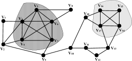
Figure 1: An example graph.

To update the core number for every node in a dynamic graph, in [20], Miorandi and Pellegrini propose to use the linear algorithm given in [8] to recompute the core number for every node in a graph. Obviously, such an algorithm is expensive when the graph is very large. In this paper, we propose a efficient algorithm to maintain the core number for each node in a dynamic network. Our algorithm is based on the following key observation. We find that only a certain number of nodes need to update their core number when a graph is updated by inserting/deleting an edge. Reconsider the example in Fig. 1. After inserting an edge $(v_{8},v_{10})$, we can observe that only the core number of the nodes $\{v_{8},v_{10},v_{18},v_{9},v_{2}\}$ updates, while the core number of the remaining nodes does not change. The key challenge is how to identify the nodes whose core numbers need to be updated. To tackle this problem, we propose a three-stage algorithm to update the core number of the nodes. First, we prove that only the core number of the nodes that are reachable from the end-nodes of the inserted/deleted edge and their core numbers equal to the minimal core number of the end-nodes may need to be updated. Based on this, we propose a coloring algorithm to find such nodes whose core numbers may need to be updated. Second, from the nodes found by the coloring algorithm, we propose a recoloring algorithm to identify the nodes whose core numbers definitely need to be updated. Third, we update the core number of such nodes by a linear algorithm. The major advantage of our algorithm is that its time complexity is independent of the graph size, and it depends on the size of the nodes found by the coloring algorithm. To further accelerate our algorithm, we develop two pruning techniques to reduce the size of the nodes found by the coloring algorithm. In addition, it is worth mentioning that our proposed algorithm can also be used to handle a batch of edge insertions and deletions by processing the edges one by one. Also, the proposed technique can be applied to process node insertions and deletions, because node insertions and node deletions can be simulated by a sequence of edge insertions and edge deletions respectively. Finally, we extensively evaluate our algorithm over 15 real-world datasets and 5 large synthetic datasets, and the results demonstrate the efficiency of our algorithm. More specifically, in real-world datasets, our algorithm reduces the average update time over the baseline algorithm from 3.2 times to 101.8 times for handling a single edge update. For handling a batch of edge updates, our algorithm needs to process the edge updates one by one, while the baseline algorithm only needs to run once for all edge updates. In the largest synthetic dataset (5 million nodes and 25 million edges), the results show that our algorithm is still more efficient than the baseline algorithm when the number of edge updates is smaller than 4700.

The rest of this paper is organized as follows. We give the problem statement in Section II. We propose our basic algorithm as well as the pruning strategies in Section III. Extensive experimental studies are reported in Section IV, and the related work is discussed in Section V. We conclude this work in Section VI.

II Preliminaries

Consider an undirected and unweighted graph $G=(V,E)$, where $V$ denotes a set of nodes and $E$ denotes a set of undirected edges between the nodes. Let $n=|V|$ and $m=|E|$ be the number of nodes and the number of edges in $G$, respectively. A graph $G^{\prime}=(V^{\prime},E^{\prime})$ is a subgraph of $G$ if $V^{\prime}\subseteq V$ and $E^{\prime}\subseteq E$. We give the definition of the $k$-core [22] as follows.

Definition 2.1: A $k$-core is the largest subgraph $G^{\prime}$ of $G$ such that each node in $G^{\prime}$ has at least a degree $k$.

The core number of node $v$ is defined as the largest $k$-core that contains this node. We denote the core number of node $v$ as $C_{v}$. It is worth noting that the nodes with a large core number are also in the low order core. That is to say, the cores are nested. For example, assuming a node $v$ is in a $3$-core, then node $v$ is also in $2$-core, $1$-core and $0$-core.

Given a graph $G$, the problem of $k$-core decomposition is to determine the core number for every node in $G$. The following example illustrates the concept of $k$-core composition in graph.

Example 2.1: Fig. 1 shows a graph $G$ that contains 18 nodes, i.e., $v_{1},\cdots,v_{18}$. By Definition II, we can find that the nodes $v_{3},\cdots,v_{7}$ form a $4$-core. The reason is because the induced subgraph by the nodes $v_{3},\cdots,v_{7}$ is the largest subgraph in which the degrees of nodes are lager than or equal to 4. Similarly, the subgraph induced by the nodes $v_{3},\cdots,v_{7},v_{14},\cdots,v_{17}$ is a $3$-core, and the whole graph $G$ is a $2$-core. Here we can find that the nodes $v_{3},\cdots,v_{7}$ are also in the $3$-core and $2$-core. $\Box$

It is well known that the $k$-core decomposition in a static graph can be calculated by a $O(n+m)$ algorithm [8]. In many applications such as online social networks, the graph evolves over time. In this paper, we consider the problem of updating the core number for every node in the graph given the graph changes over time. In this problem, we assume that the core numbers of all the nodes have been known before the graph is updated. The potential change in our problem is that either edge insertion or edge deletion may result in the core number of a number of nodes that needs to be updated. Previous solution for this problem [20] is to perform the $O(n+m)$ core decomposition algorithm to re-compute the core number for every node in the updated graph. Clearly, such algorithm is expensive when the graph is very large. In the following, we mainly focus on devising more efficient algorithm for $k$-core decomposition in a graph given the graph is updated by an edge insertion or deletion. Our proposed algorithm can also be used for processing a batch of edge updates. Moreover, since node insertions and deletions can be easily simulated as a sequence of edge insertions and edge deletions respectively, our algorithm can also be applied to handle node insertions and node deletions.

III The proposed algorithm

Let $N(v)$ be the set of neighbor nodes of node $v$, $D_{v}$ be the degree of node $v$, i.e., $D_{v}=|N(v)|$. Then, we give two important quantities associated with a node $v$ as follows. Specifically, we define $X_{v}$ as the number of $v$’s neighbors whose core numbers are greater than or equal to $C_{v}$, and define $Y_{v}$ as the number of $v$’s neighbors whose core numbers are strictly greater than $C_{v}$. Formally, for a node $v$, we have $X_{v}=|\{u:u\in N(v),C_{u}\geq C_{v}\}|$ and $Y_{v}=|\{u:u\in N(v),C_{u}>C_{v}\}|$. In effect, by definition, $X_{v}$ denotes the degree of node $v$ in the $C_{v}$-core. The following lemma shows that $C_{v}$ is bounded by $Y_{v}$ and $X_{v}$.

Lemma 3.1: For every node $v$ of a graph $G$, we have $Y_{v}\leq C_{v}\leq X_{v}\leq D_{v}$.

Proof: We denote the subgraph $G^{\prime}=(V^{\prime},E^{\prime})$ as the $C_{v}$-core. Obviously, node $v$ is in $G^{\prime}$. By Definition II, in $G^{\prime}$, node $v$ has at least $C_{v}$ neighbors, and the core number of all the nodes in $G^{\prime}$ is at least $C_{v}$. In other words, the number of $v$’s neighbors whose core numbers are larger than or equal to $C_{v}$ is at least $C_{v}$. By definition, $X_{v}$ denotes such number. Therefore, we have $C_{v}\leq X_{v}$. In addition, by definition, we clearly know that $X_{v}\leq D_{v}$. For $Y_{v}\leq C_{v}$, we can prove it by contradiction. Suppose $Y_{v}>C_{v}$, then node $v$ has more than $C_{v}$ neighbors whose core numbers are strictly greater than $C_{v}$. By Definition II, the core number of node $v$ should be at least $C_{v}+1$, which is a contradiction. This completes the proof. $\Box$

In the following, we give an example to illustrate the concepts of $X_{v}$ and $Y_{v}$.

Example 3.1: Consider the node $v_{9}$ in Fig. 1. By definition, the core number of node $v_{9}$ is 2, i.e., $C_{v_{9}}=2$, and the degree of $v_{9}$ equals to 3, i.e., $D_{v_{9}}$=3. Node $v_{9}$ has three neighbors ($v_{2},v_{7}$, and $v_{10}$) whose core number is greater than or equal to 2, and has one neighbor ($v_{7}$) whose core number is strictly greater than 2. Therefore, we have $X_{v_{9}}=3$ and $Y_{v_{9}}=1$, which consists with Lemma III. Similar results can be observed from other nodes in Fig. 1. $\Box$

Below, we define the notion of induced core subgraph.

Definition 3.1: Given a graph $G=(V,E)$ and a node $v$, the induced core subgraph of node $v$, denoted as $G_{v}=(V_{v},E_{v})$, is a connected subgraph which consists of node $v$. Moreover, the core number of all the nodes in $G_{v}$ is equivalent to $C_{v}$.

By Definition III, the induced core subgraph of node $v$ includes the nodes such that they are reachable from $v$ and their core numbers equal to $C_{v}$. Based on Definition III, we define the union of two induced core subgraphs.

Definition 3.2: For two nodes $u$ and $v$ and their corresponding induced core subgraph $G_{u}=(V_{u},E_{u})$ and $G_{v}=(V_{v},E_{v})$, the union of $G_{u}$ and $G_{v}$ is defined as $G_{u\cup v}=(V_{u\cup v},E_{u\cup v})$, where $V_{u\cup v}=V_{v}\bigcup V_{u}$ and $E_{u\cup v}=\{(v_{i},v_{j})|(v_{i},v_{j})\in E,v_{i}\in V_{u\cup v},v_{j}\in V_{u\cup v}\}$.

It is worth mentioning that the union of two induced core subgraphs may not be connected. The following example illustrates the definitions of induced core subgraph and union of two induced core subgraphs.

Example 3.2: Consider the nodes $v_{8}$ and $v_{10}$ in Fig. 1. By definition, the induced core subgraph of $v_{8}$ is a subgraph that only contains node $v_{8}$. That is to say, $V_{v_{8}}=\{v_{8}\}$ and $E_{v_{8}}=\emptyset$. The induced core subgraph of node $v_{10}$ is a subgraph that includes nodes $\{v_{1},v_{2},v_{9},v_{10},v_{11},v_{12},v_{13},v_{18}\}$. In other words, $V_{v_{10}}=\{v_{1},v_{2},v_{9},v_{10},v_{11},v_{12},v_{13},v_{18}\}$ and $E_{v_{10}}=\{(v_{1},v_{2}),(v_{2},v_{9}),(v_{9},v_{10}),(v_{10},v_{11}),(v_{10},v_{18}),(v_{11},v_{12}),\\ (v_{11},v_{13})\}$. The union of these two induced core subgraphs is $G_{v_{8}\cup v_{10}}=(V_{v_{8}\cup v_{10}},E_{v_{8}\cup v_{10}})$, where $V_{v_{8}\cup v_{10}}=\{v_{1},v_{2},v_{8},v_{9},v_{10},v_{11},v_{12},v_{13},v_{18}\}$ and $E_{v_{8}\cup v_{10}}=E_{v_{10}}$. Fig. 2 illustrates the union of two induced core subgraphs $G_{v_{8}\cup v_{10}}$. $\Box$

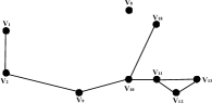
Figure 2: The union of two induced core subgraphs ($G_{v_{8}\cup v_{10}}$).

Based on Definition III and III, we give a $k$-core update theorem.

Theorem 3.1: ($k$-core update theorem) Given a graph $G=(V,E)$ and two nodes $u$ and $v$.

• If $C_{u}>C_{v}$, then either insertion or deletion of an edge $(u,v)$ in $G$, only the core number of nodes in the induced core subgraph of node $v$, i.e., $G_{v}$, may need to be updated.

• IF $C_{u}<C_{v}$, then either insertion or deletion of an edge $(u,v)$ in a graph $G$, only the core number of nodes in the induced core subgraph of node $u$, i.e., $G_{u}$, may need to be updated.

• IF $C_{u}=C_{v}$, then either insertion or deletion of an edge $(u,v)$ in a graph $G$, only the core number of nodes in the union of two induced core subgraphs $G_{u}$ and $G_{v}$, i.e., $G_{u\cup v}$, may need to be updated.

To prove Theorem 2, we first give some useful lemmas as follows.

Lemma 3.2: Given a graph $G=(V,E)$ and a node $u$. If the core number of node $u$’s neighbors increases (decreases) by at most 1, then $C_{u}$ increases (decreases) by at most 1.

Proof: First, we prove the increase case by contradiction. Suppose that $C_{u}$ increases by at least 2. This implies that there are at least $C_{u}+2$ neighbors of node $u$ whose core numbers are larger than or equal to $C_{u}+2$. Since the core number of $u$’s neighbors increases by at most 1, the number of $u$’s neighbors whose core numbers are larger than or equal to $C_{u}+2$ is at most $Y_{u}$. By Lemma III, we know that $Y_{u}\leq C_{u}$. That is to say, the number of $u$’s neighbors whose core numbers are larger than or equal to $C_{u}+2$ is bounded by $C_{u}$, which is a contradiction.

Second, we prove the decrease case. If the core number of the neighbors of node $u$ decreases by at most 1, then $u$ has at least $X_{u}$ neighbors whose core numbers are greater than or equal to $C_{u}-1$. Since $X_{u}\geq C_{u}>C_{u}-1$, the core number of node $u$ is at least $C_{u}-1$. Therefore, $C_{u}$ decreases by at most 1. This completes the proof. $\Box$

Lemma 3.3: If we insert (delete) an edge $(u,v)$ in a graph $G$, the core number of any node in $G$ increases (decreases) by at most 1.

Proof: We focus on proving the edge insertion case, and similar arguments can be used to prove the edge deletion case. After inserting an edge $(u,v)$, both $D_{u}$ and $D_{v}$ increase by 1. Recall that $X_{u}$ ($X_{v}$) denotes the degree of $u$ ($v$) in the $C_{u}$-core ($C_{v}$-core), which is a subgraph of $G$. Therefore, $X_{u}$ and $X_{v}$ increase by at most 1. By definition, $C_{u}$ ($C_{v}$) equals to the minimal degree of the nodes in the $C_{u}$-core ($C_{v}$-core). Since $X_{u}$ ($X_{v}$) increases by at most 1, the minimal degree of the nodes in the $C_{u}$-core ($C_{v}$-core) increases by at most 1. As a result, the core number of node $u$ ($v$) increases by at most 1. Such increase of $C_{u}$ ($C_{v}$) may lead to increasing the core number of the neighbors of node $u$ ($v$). Consider the one-hop neighbors of node $u$ ($v$). According to Lemma 2, the core number of all the neighbors of node $u$ ($v$) increases by at most 1. By recursively applying Lemma 2, we can conclude that the core number of all the nodes that are reachable from $u$ ($v$) increases by at most 1. On the other hand, the core number of the nodes that cannot be reachable from $u$ ($v$) does not change. Put it all together, for any node in $G$, its core number increases by at most 1. This completes the proof. $\Box$

Lemma 3.4: Given a graph $G$ and two nodes $u$ and $v$ such that $C_{u}=C_{v}$. If we insert an edge $(u,v)$ in $G$, then either $C_{u}$ and $C_{v}$ increase by 1 or $C_{u}$ and $C_{v}$ do not change.

Proof: We prove it by contradiction. Without loss of generality, after inserting an edge $(u,v)$, we assume that $C_{u}$ increases by 1 while $C_{v}$ does not change. Since $C_{u}$ increases by 1, node $u$ has at least $C_{u}+1$ neighbors whose core numbers are larger than or equal to $C_{u}+1$. By Definition II, before inserting an edge $(u,v)$, $u$ has at most $C_{u}$ neighbors whose core numbers are larger than or equal to $C_{u}+1$. Therefore, node $v$’s core number must be $C_{u}+1$, which is a contradiction.

Lemma 3.5: Given a graph $G$ and an edge $(u,v)$. Suppose $G$ is updated by inserting or deleting an edge $(u,v)$. Then, for any node $w$ in $G$, if the core number of $w$ ($C_{w}$) needs to be changed, such change only affects the core number of nodes in $G_{w}$. If $C_{w}$ does not change, then it does not affect the core number of the nodes in $G$.

Proof: We focus on the edge insertion case, and similar proof can be used to prove the edge deletion case. Assume that $C_{w}$ is changed after inserting an edge $(u,v)$ into $G$. By Lemma 2, $C_{w}$ increases by 1. We denote the updated $C_{w}$ as $\tilde{C}_{w}$, i.e., $\tilde{C}_{w}=C_{w}+1$. Obviously, the increase of $C_{w}$ does not affect the core number of the nodes that cannot be reachable from $w$. Also, we claim that the increase of $C_{w}$ does not affect the core numbers of the nodes that can be reachable from $w$ and their core numbers are less than or greater than $C_{w}$. First, we consider a node $z$ that are reachable from $w$ and $C_{z}<C_{w}$. Recall that $C_{z}$ equals to the minimal degree of the nodes in the $C_{z}$-core. By definition, $w$ is also in the $C_{z}$-core (cores are nested). The increase of $C_{w}$ clearly does not increase such minimal degree. Hence, the core number of node $z$ is still $C_{z}$. Second, we consider a node $z$ that is reachable from $w$ and $C_{z}>C_{w}$. The minimal degree of the nodes in $C_{z}$-core is $C_{z}$ and $C_{z}\geq\tilde{C}_{w}$. Similarly, the increase of $C_{w}$ does not increase such minimal degree, thereby $C_{z}$ will not be updated. Put it all together, the increase of $C_{w}$ only affects the core number of those nodes that are reachable from $w$ and their core numbers equal to $C_{w}$, which are the nodes in $G_{w}$. By definition, if $C_{w}$ does not change, then it will not affect the core number of all the nodes in $G$. This completes the proof. $\Box$

Armed with the above lemmas, we prove the $k$-core update theorem as follows.

Proof of Theorem 2: For the insertion of an edge $(u,v)$, we consider three different cases: (1) $C_{u}>C_{v}$, (2) $C_{u}<C_{v}$, and (3) $C_{u}=C_{v}$. For $C_{u}>C_{v}$, we know that node $u$ is in a higher order core than node $v$. By Definition II, adding a neighbor $v$ with a small core number to a node $u$ does not affect $C_{u}$. By Lemma 2, since $C_{u}$ does not change, node $u$ will not affect the core number of the nodes in $G$. Consequently, we only need to update the core number of the nodes that are affected by node $v$. By Lemma 2, if $C_{v}$ changes, then only the core number of nodes in $G_{v}$ may need to be updated. If $C_{v}$ does not change, then no node’s core number needs to be updated. This proves the case (1). Symmetrically, we can use the similar arguments to prove the case (2). For case (3), after inserting an edge $(u,v)$, by Lemma 2, either $C_{u}$ and $C_{v}$ increase by 1 or $C_{u}$ and $C_{v}$ do not change. If $C_{u}$ and $C_{v}$ do not change, by Lemma 2, we conclude that no node’s core number needs to be updated. If $C_{u}$ and $C_{v}$ increase by 1, by Lemma 2, the core number of the nodes in $G_{u}$ and $G_{v}$ may need to be updated. That is to say, the core number of the nodes in $G_{u\cup v}$ may need to be updated.

Similarly, for the deletion of an edge $(u,v)$, we also consider three different cases: (1) $C_{u}>C_{v}$, (2) $C_{u}<C_{v}$, and (3) $C_{u}=C_{v}$. The proof for the first two cases is very similar to the proof for the first two cases under edge insertion case, thereby we omit for brevity. For $C_{u}=C_{v}$, after deleting an edge $(u,v)$, if $C_{u}$ and $C_{v}$ do not change, we conclude that no node’s core number needs to be updated according to Lemma 2. If $C_{u}$ changes, by Lemma 2, the core number of nodes in $G_{u}$ may need to be updated. Likewise, if $C_{v}$ changes, the core number of nodes in $G_{v}$ may need to be updated. To summarize, after removing an edge $(u,v)$, only the core number of the nodes in $G_{u\cup v}$ may need to be updated. This completes the proof. $\Box$

III-A The basic algorithm

In this subsection, we present a basic algorithm for core maintenance in a graph given the graph is updated by an edge insertion or an edge deletion. Below, we describe the detailed algorithms for edge insertion and deletion, respectively.

Algorithm for edge insertion: Our main algorithm for edge insertion consists of three steps. After inserting an edge $(u,v)$, by the $k$-core update theorem, only the core number of nodes in the induced core subgraph ($G_{u}$ or $G_{v}$ or $G_{u\cup v}$) may need to be updated. Therefore, the first step of our main algorithm is to identify the nodes in the induced core subgraph. Let $V_{c}$ be the set of nodes found in the first step. Then, the second step of our algorithm is to determine those nodes in $V_{c}$ whose core numbers definitely need to be updated. Finally, the third step of our algorithm is to update the core number of such nodes.

Our main algorithm for edge insertion, called Insertion, is outlined in Algorithm 1. Algorithm 1 includes three sub-algorithms, namely Color, RecolorInsert, and UpdateInsert, which corresponds the first, the second, and the third step of our main algorithm, respectively. In particular, Color is used to color the nodes in $V_{c}$ with a color 1, RecolorInsert is applied to recolor the nodes in $V_{c}$ whose core numbers are definitely unchanged with a color 0, and UpdateInsert is used to update the core number of the nodes in $V_{c}$ with a color 1. The detailed description of Algorithm 1 is as follows. First, Algorithm 1 assigns a color 0 for every node in $G$ (line 2 in Algorithm 1) and initializes $V_{c}$ by an empty set (line 3 in Algorithm 1). Second, the algorithm updates the core number of the nodes under three different cases, i.e., $C_{u}>C_{v}$, $C_{u}<C_{v}$, and $C_{u}=C_{v}$. Specifically, under the first case ($C_{u}>C_{v}$), the algorithm first invokes Color($G$, $v$, $c$) to find the nodes in $G_{v}$ (line 6 in Algorithm 1), because only the core number of the nodes in $G_{v}$ may need to be updated. After this process, all the nodes in $G_{v}$ are recorded in $V_{c}$ and all of them are colored by 1. Then, the algorithm invokes RecolorInsert($G$, $c$) to identify the nodes whose core numbers are definitely unchanged (line 7 in Algorithm 1). After this step, all of such nodes in $V_{c}$ are recolored by 0. Finally, the algorithm invokes UpdateInsert($G$, $c$) to update the core number of the nodes in $V_{c}$ with color 1 (line 8 in Algorithm 1). Similar process can be used for other two cases (line 9-13 in Algorithm 1). Note that for the case $C_{u}=C_{v}$, we can invoke Color($G$, $u$, $c$) to find the nodes in $G_{u\cup v}$, because $u$ can reach $v$ after inserting an edge $(u,v)$. Below, we describe the details of our sub-algorithms, Color, RecolorInsert, and UpdateInsert, respectively.

Algorithm 1 Insertion($G$, $u$, $v$)

Input:	Graph $G=(V,E)$ and an edge $(u,v)$
Output: the updated core number of the nodes

1:  Initialize visited($w$) $\leftarrow 0$ for all node $w\in V$;

2:  Initialize color($w$) $\leftarrow 0$ for all node $w\in V$;

3:  $V_{c}\leftarrow\emptyset$;

4:  if $C_{u}$ $>C_{v}$ then

5:     $c\leftarrow C_{v}$;

6:     Color($G$, $v$, $c$);

7:     RecolorInsert($G$, $c$);

8:     UpdateInsert($G$, $c$);

9:  else

10:     $c\leftarrow C_{u}$;

11:     Color($G$, $u$, $c$);

12:     RecolorInsert($G$, $c$);

13:     UpdateInsert($G$, $c$);

Algorithm 2 void Color($G$, $u$, $c$)

1:  visited($u$) $\leftarrow 1$;

2:  if color($u$) = 0 then

3:     $V_{c}\leftarrow V_{c}\cup\{u\}$;

4:     color($u$) = 1;

5:  for each node $w\in N(u)$ do

6:     if visited($w$) $=0$ and $C_{w}=c$ then

7:        Color($G$, $w$, $c$);

Algorithm 3 void RecolorInsert($G$, $c$)

1:  flag $\leftarrow 0$;

2:  for each node $u\in V_{c}$ do

3:     if color($u$) = 1 then

4:        $X_{u}\leftarrow 0$;

5:        for each node $w\in N(u)$ do

6:           if (color($w$) = 1) or ($C_{w}>c$) then

7:              $X_{u}\leftarrow X_{u}+1$;

8:        if $X_{u}\leq c$ then

9:           color($u$) $\leftarrow 0$;

10:           flag $\leftarrow 1$;

11:  if flag = 1 then

12:     RecolorInsert($G$, $c$);

Algorithm 4 void UpdateInsert($G$, $c$)

1:  for each node $w\in V_{c}$ do

2:     if color($w$) $=1$ then

3:        $C_{w}\leftarrow c+1$;

Recall that after inserting an edge $(u,v)$, by the $k$-core update theorem, we have three cases that need to be considered, i.e., $C_{u}<C_{v}$, $C_{u}>C_{v}$, and $C_{u}=C_{v}$. To simplify our description, we mainly focus on describing our sub-algorithms under the case $C_{u}=C_{v}$, and similar description can be used for other cases. Suppose that node $u$ and $v$ have core number $C_{u}=C_{v}=c$. In this case, we have $V_{c}=V_{u\cup v}$. By Definition III, finding the nodes in $V_{u\cup v}$ can be done by a Depth-First-Search (DFS) algorithm. Color depicted in Algorithm 2 is indeed such a DFS algorithm. In particular, Color will assign a color 1 to every node in $V_{c}$. At the beginning, $V_{c}$ is initialized by an empty set and all the nodes are associated with a color 0. The algorithm recursively finds the nodes that are reachable from $u$ and have core number $c$ (line 6-7 in Algorithm 2). When the algorithm visits such a node, if its color is 0, then the algorithm colors it by 1 and adds it into the set $V_{c}$ (line 3-4 in Algorithm 2). To find all the nodes in $V_{u\cup v}$, we can invoke Color($G$, $u$, $c$). Recall that after inserting edge $(u,v)$, the nodes that are reachable from $v$ can also be found by Color($G$, $u$, $c$).

RecolorInsert described in Algorithm 3 is used to identify the nodes in $V_{c}$ whose core numbers are definitely unchanged. Specifically, Algorithm 3 recursively recolors the nodes whose core numbers do not change by a color 0. The recursion is terminated until no node needs to be recolored. In each recursion, the algorithm re-computes $X_{u}$ for each node $u$ in $V_{c}$. Here the recomputed $X_{u}$ equals to the sum of the number of neighbors of node $u$ whose core numbers are larger than $c$ and the number of neighbors of node $u$ with color 1 (line 4-7 in Algorithm 3). For a node $u$, if the current $X_{u}$ is smaller than or equal to $c$, then the algorithm recolors it by 0 (line 8-10 in Algorithm 3).

The rationale of Algorithm 3 is as follows. First, Algorithm 3 assumes that the core numbers of all the nodes in $V_{c}$ need to be updated. Then, for each node $w$ in $V_{c}$, the algorithm recomputes $X_{w}$. Initially, since all the neighbors of $w$ whose core numbers equal to $c$ are colored by 1, $X_{w}$ is indeed the same value as our previous definition. If $X_{w}\leq c$, then $w$ at most $c$ neighbors whose core numbers are larger than $c$ after inserting an edge $(u,v)$. As a result, $C_{w}$ cannot be updated and the algorithm recolors it by 0. This recoloring process may affect the color of $w$’s neighbors. The reason is because, before recoloring $w$, $w$ may contribute to calculate $X_{z}$, where $z$ is a neighbor of $w$. Consequently, the algorithm needs to recursively recolor the nodes in $V_{c}$. Note that Algorithm 3 is recursively invoked at most $|V_{c}|+1$ times, because the algorithm at least recolors one node at a recursion in the worse case. The following theorem shows that after Algorithm 3 terminates, a node with a color 1 is a sufficient and necessary condition for updating its core number.

Theorem 3.2: Under the case of insertion of an edge $(u,v)$, the core number of a node needs to be updated if and only if its color is 1 after Algorithm 3 terminates.

Proof: First, we prove that if the core number of a node $w$ needs to be updated, then its color is 1 after Algorithm 3 terminates. We focus on the case of $C_{u}=C_{v}=c$, similar proof can be used to prove the other two cases. By our assumption and Lemma 2, we have $w\in V_{c}$, where $V_{c}=V_{u\cup v}$. Then, by Lemma 2, after inserting an edge $(u,v)$, the core number of the nodes in $V_{c}$ increases by at most 1. Therefore, if $C_{w}$ needs to be updated, then the updated core number of $w$ must be $c+1$. That is to say, node $w$ must have $c+1$ neighbors whose core numbers are larger than or equal to $c+1$. Now assume that the color of node $w$ is 0. This means that $X_{w}\leq c$ when Algorithm 3 terminates. Recall that $X_{w}$ denotes to the sum of the number of neighbors whose core numbers are larger than $c$ and the number of neighbors whose color is 1. This implies that node $w$ has at most $c$ neighbors whose core numbers are larger than $c$, which is a contradiction.

Second, we prove that if a node has a color 1 after Algorithm 3 terminates, then the core number of this node must be updated. We consider the induced subgraph by the nodes with color 1 after Algorithm 3 terminates and the nodes whose core numbers are greater than $c$. Consider a node $w$ in such an induced subgraph. Clearly, if $w$ has a color 1, then it has $X_{w}>c$ neighbors. And if $w$ has a color 0, then its core number $C_{w}$ is larger than $c$. By Definition II, the induced subgraph belongs to the $(c+1)$-core. Therefore, the core number of a node $w$ with color 1 is at least $c+1$. By Lemma 2, after inserting an edge $(u,v)$, the core number of any nodes in graph $G$ increases by at most 1. Consequently, the core number of the nodes with color 1 increases by 1. This completes the proof. $\Box$

UpdateInsert outlined in Algorithm 4 increases the core numbers of the nodes in $V_{c}$ with label 1 to $c+1$, because only the core numbers of those nodes need to increase by 1 after the coloring and recoloring processes. The correctness of our algorithm for edge insertion can be guaranteed by Theorem 2 and Theorem 4. The following example explains how the Insertion algorithm works.

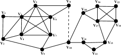
Figure 3: A graph after inserting an edge $(v_{8},v_{10})$.

Example 3.3: Let us consider the same graph given in Fig. 1. Assume that we insert an edge $(v_{8},v_{10})$, which results in a graph given in Fig. 3. In Fig. 3, the dashed line denotes the inserted edge. Since $C_{v_{8}}=C_{v_{10}}=c=2$, the Insertion algorithm first invokes Color($G$, $v_{8}$, $2$). After this process, we can get that $V_{c}=\{v_{8},v_{10},v_{9},v_{2},v_{1},v_{18},v_{11},v_{12},v_{13}\}$. And all the nodes in $V_{c}$ are colored by 1 and the other nodes are colored by 0. Then, the algorithm invokes the RecolorInsert($G$, $2$) algorithm. To simplify our description, we assume that the node visiting-order in $V_{c}$ is their DFS visiting-order. At the first recursion, we can find that $X_{v_{1}}=2$, thereby it is recolored by 0. Also, the node $V_{12}$ is recolored by 0, because $X_{v_{12}}=2$. At the second recursion, we can find that the nodes $v_{11}$ and $v_{13}$ are recolored by 0. At the third recursion, no node needs to be recolored, the algorithm therefore terminates. After invoking the RecolorInsert($G$, $2$) algorithm, the nodes $\{v_{8},v_{10},v_{9},v_{2},v_{18}\}$ are colored by 1, thereby their core numbers must increase to 3 by Theorem 4. Finally, the Insertion algorithm invokes the UpdateInsert($G$, $2$) algorithm to update the core number of such nodes. As a consequence, the core number of the nodes $\{v_{8},v_{10},v_{9},v_{2},v_{18}\}$ is increased to 3. $\Box$

We analyze the time complexity of the Insertion algorithm as follows. First, the Color algorithm takes $O(\sum\nolimits_{u\in V_{c}}{D_{u}})$ time complexity. Second, the RecolorInsert algorithm takes $O(|V_{c}|\sum\nolimits_{u\in V_{c}}{D_{u}})$ time complexity in the worse case, as the algorithm is recursively invoked at most $O(|V_{c}|)$ times and each recursion takes $O(\sum\nolimits_{u\in V_{c}}{D_{u}})$ time complexity. Finally, the UpdateInsert algorithm takes $O(|V_{c}|)$ time complexity. Put it all together, the time complexity of the Insertion algorithm is $O(|V_{c}|\sum\nolimits_{u\in V_{c}}{D_{u}})$ in the worse case, which is independent of the graph size. However, in practice, the algorithm is more efficient than such worse-case time complexity. The reason could be of twofold. On the one hand, $|V_{c}|$ typically not very large w.r.t. the number of nodes of the graph. On the other hand, very often, the RecolorInsert algorithm terminates very fast.

Algorithm for edge deletion: The main algorithm for edge deletion, namely Deletion, is outlined in Algorithm 5. Similar to the edge insertion case, Deletion also includes three sub-algorithms: Color, RecolorDelete, and UpdateDelete. Here Color is used to find the nodes in the induced core subgraph, RecolorDelete is utilized to identify the nodes whose core numbers need to be updated, and UpdateDelete is applied to update the core numbers of the nodes identified by RecolorDelete. The detailed description of Deletion is given as follows.

Similarly, let $V_{c}$ be a set of nodes whose core numbers may need to be updated. First, Algorithm 5 initializes the color of all the nodes to 0 and $V_{c}$ to an empty set. Likewise, under the edge deletion case, we also have to consider three cases. That is, $C_{u}>C_{v}$, $C_{u}<C_{v}$, and $C_{u}=C_{v}$. If $C_{u}>C_{v}$, only the core number of the nodes in $G_{v}$ may need to be updated. Under this case, the algorithm invokes Color($G$, $v$, $c$) to find the nodes in $V_{c}$ (line 6 in Algorithm 5). Then, the algorithm invokes RecolorDelete($G$, $c$) to identify the nodes whose core numbers need to be changed (line 7 in Algorithm 5). Finally, the algorithm invokes UpdateDelete($G$, $c$) to update the core number of such nodes (line 8 in Algorithm 5). Similar process can be used for the $C_{u}<C_{v}$ case. For the $C_{u}=C_{v}$ case, the algorithm first invokes Color($G$, $u$, $c$) to find the nodes in $G_{u}$ (line 16 in Algorithm 5). Then, the algorithm has to handle two different cases. First, if $u$ can reach $v$, then the coloring algorithm can also find the nodes in $G_{v}$ (in this case, $v$’s color is 1, line 22 in Algorithm 5). Second, if $u$ cannot reach $v$ ($v$’s color is 0), then the algorithm invokes Color($G$, $v$, $c$) to find the nodes in $G_{v}$ (line 19 in Algorithm 5). After this process, all the node in $G_{u\cup v}$ are recorded in $V_{c}$. Then, we can invoke RecolorDelete($G$, $c$) and UpdateDelete($G$, $c$) algorithms to update the core number of the nodes in $V_{c}$. Below, we give the detailed descriptions of RecolorDelete and UpdateDelete respectively.

Algorithm 5 Deletion($G$, $u$, $v$)

Input:	Graph $G=(V,E)$ and an edge $(u,v)$
Output: the updated core number of the nodes

1:  Initialize visited($w$) $\leftarrow 0$ for all node $w\in V$;

2:  Initialize color($w$) $\leftarrow 0$ for all node $w\in V$;

3:  $V_{c}\leftarrow\emptyset$;

4:  if $C_{u}$ $>C_{v}$ then

5:     $c\leftarrow C_{v}$;

6:     Color($G$, $v$, $c$);

7:     RecolorDelete($G$, $c$);

8:     UpdateDelete($G$, $c$);

9:  if $C_{u}$ $<C_{v}$ then

10:     $c\leftarrow C_{u}$;

11:     Color($G$, $u$, $c$);

12:     RecolorDelete($G$, $c$);

13:     UpdateDelete($G$, $c$);

14:  if $C_{u}$ $=C_{v}$ then

15:     $c\leftarrow C_{u}$;

16:     Color($G$, $u$, $c$);

17:     if color($v$) $=0$ then

18:        Initialize visited($w$) $\leftarrow 0$ for all node $w\in V$;

19:        Color($G$, $v$, $c$);

20:        RecolorDelete($G$, $c$);

21:        UpdateDelete($G$, $c$);

22:     else

23:        RecolorDelete($G$, $c$);

24:        UpdateDelete($G$, $c$);

Algorithm 6 void RecolorDelete($G$, $c$)

1:  flag $\leftarrow 0$;

2:  for each node $u\in V_{c}$ do

3:     if color($u$) = 1 then

4:        $X_{u}\leftarrow 0$;

5:        for each node $w\in N(u)$ do

6:           if (color($w$) = 1) or ($C_{w}>c$) then

7:              $X_{u}\leftarrow X_{u}+1$;

8:        if $X_{u}<c$ then

9:           color($u$) $\leftarrow 0$;

10:           flag $\leftarrow 1$;

11:  if flag = 1 then

12:     RecolorDelete($G$, $c$);

Algorithm 7 void UpdateDelete($G$, $c$)

1:  for each node $w\in V_{c}$ do

2:     if color($w$) $=0$ then

3:        $C_{w}\leftarrow c-1$;

Similar to the edge insertion case, after invoking Color, the nodes whose core numbers may need to be updated are recorded in a set $V_{c}$, and also all of them are colored by 1. After obtaining the set $V_{c}$, RecolorDelete described in Algorithm 6 is used to determine the nodes whose core numbers must be updated. In particular, RecolorDelete recursively recolors the nodes whose core numbers need to be updated by 0. In each recursion, the algorithm calculates $X_{w}$ for every node $w$ in $V_{c}$. Here $X_{w}$ denotes the sum of the number of $w$’s neighbors whose color is 1 and the number of $w$’s neighbors whose core numbers are larger than $c$, where $c=\min\{C_{u},C_{v}\}$. For a node $w\in V_{c}$, if $X_{w}<c$, then the algorithm colors $w$ by 0. The algorithm terminates if no node needs to be recolored. Clearly, the algorithm is invoked at most $|V_{c}|$ times. The following theorem shows that a node in $V_{c}$ with a color 0 after Algorithm 6 terminates is a sufficient and necessary condition for updating its core number.

Theorem 3.3: Under the case of deletion of an edge $(u,v)$, a node in $V_{c}$ whose core number needs to update if and only if its color is 0 after Algorithm 6 terminates.

Proof: First, we prove that if a node $w$ in $V_{c}$ whose core number needs to be updated, then its color is 0 after Algorithm 6 terminates. By our assumption and Lemma 2, after deleting an edge $(u,v)$, $C_{w}$ decreases by 1. This means that $C_{w}$ decreases to $c-1$. That is to say, $w$ has $c-1$ neighbors whose core numbers are larger than or equal to $c-1$. Suppose that the color of $w$ is 1 after the algorithm terminates. This implies that $X_{w}\geq c$. Recall that $X_{w}$ denotes the sum of the number of $w$’s neighbors whose core numbers are lager than $c$ and the number of $w$’s neighbors whose color is 1. Note that a node with color 1 suggests that its core number equals to $c$. As a result, $w$ has at least $c$ neighbors whose core numbers are larger than or equal to $c$, which is a contradiction.

Second, we prove that if a node $w$ in $V_{c}$ is recolored by 0 after Algorithm 6 terminates, then $C_{w}$ must be updated. After deleting an edge $(u,v)$, we construct an induced subgraph, which is denoted as $\tilde{G}=(\tilde{V},\tilde{E})$, by the nodes in $V_{c}$ and the nodes whose core numbers are larger than $c$. Note that the core number of the nodes in $V\backslash\tilde{V}$ is smaller than $c$. Therefore, they do not affect the core number of the nodes in $\tilde{V}$. If a node $w\in V_{c}$ with a color 0 after Algorithm 6 terminates, then $X_{w}<c$. This suggests that the node $w$ in $\tilde{G}$ has at most $c-1$ neighbors. By Definition II, $\tilde{G}$ at most belongs to the $(c-1)$-core. By Lemma 2, the core number of any nodes in $G$ decreases by at most 1 after deleting an edge. Therefore, the core number of the nodes with color 0 decreases by 1. This completes the proof. $\Box$

UpdateDelete which is depicted in Algorithm 7 is used to update the core number of the nodes in $V_{c}$ with color 0 to $c-1$, because only the core numbers of those nodes need to decrease by 1 after the coloring and recoloring steps. The correctness of Deletion can be guaranteed by Theorem 2 and Theorem 7. By a similar analysis as the edge insertion case, the time complexity of Deletion($G$, $u$, $v$) is $O(|V_{c}|\sum\nolimits_{u\in V_{c}}{D_{u}})$. The following example explains how Deletion works.

Example 3.4: Let’s consider the graph depicted in Fig. 3. Suppose that we delete the edge $(v_{8},v_{10})$. Since $C_{v_{8}}=C_{v_{10}}=c=3$, the Deletion algorithm first invokes Color($G$, $v_{8}$, $3$), which results in $V_{c}=\{v_{8}\}$. Clearly, the color of $v_{10}$ is 0 after this process ends. Hence, the algorithm invokes Color($G$, $v_{10}$, $3$), which leads to $V_{c}=\{v_{8},v_{10},v_{9},v_{2},v_{18}\}$. After this process, all the nodes in $V_{c}$ are colored by 1 and other nodes are colored by 0. Then, the algorithm invokes RecolorDelete($G$, $3$). At the first recursion, since $X_{v_{8}}=2$, $v_{8}$ is recolored by 0. Similarly, $v_{10},v_{9},v_{2}$, and $v_{18}$ will be recolored by 0 at the first recursion. At the second recursion, the algorithm terminates because no node needs to be recolored. Therefore, all the nodes in $V_{c}$ are recolored by 0. Finally, the algorithm invokes UpdateDelete($G$, $c$) to decrease the core number of all the nodes in $V_{c}$ to 2. $\Box$

III-B Pruning strategies

As analysis in the previous subsection, the time complexity of our Insertion and Deletion algorithms depend on the size of $V_{c}$. In this subsection, to further accelerate our algorithms, we devise two pruning techniques, namely $X$-pruning and $Y$-pruning, to remove the nodes in $V_{c}$ whose core numbers are definitely unchanged given the graph is updated.

$X$-pruning: By Lemma III, for a node $w$, $X_{w}$ is an upper bound of $C_{w}$. Here we make use of such upper bound to develop pruning technique. We refer to it as $X$-pruning. Below, we discuss the $X$-pruning technique over the edge insertion and edge deletion cases, respectively.

First, we consider the insertion case. Assume that we insert an edge $(u_{0},v_{0})$. Also, we need to consider three cases, $C_{u_{0}}>C_{v_{0}}$, $C_{u_{0}}<C_{v_{0}}$, $C_{u_{0}}=C_{v_{0}}$. Below, we mainly focus on describing the $X$-pruning rule under the case of $C_{u_{0}}=C_{v_{0}}$, and similar descriptions can be used for other two cases. For a node $w$ in $V_{c}$, after inserting an edge $(u_{0},v_{0})$, if $X_{w}$ equals to $c$, then $C_{w}$ cannot increases to $c+1$. As a result, we can safely prune $w$. For example, consider an graph in Fig. 3. Assume that we insert an edge $(v_{8},v_{10})$. Then, for the node $v_{1}$, we have $X_{v_{1}}=2$. Clearly, $C_{v_{1}}$ cannot increase to 3, thereby we can prune $v_{1}$.

In effect, after removing $w$, for the nodes that cannot be reachable from $u_{0}$ and $v_{0}$ in the induced core subgraph can also be pruned. Let us consider a toy induced subgraph shown in Fig. 4. Suppose that the induced subgraph can be partitioned into three parts, $S_{1}$, $w$, and $S_{2}$. Further, we assume that both $u_{0}$ and $v_{0}$ are in $S_{1}$, and $X_{w}=c$. Recall that after inserting an edge $(u_{0},v_{0})$, if $X_{w}=c$, then $C_{w}$ is unchanged. By Lemma 2, $w$ will not affect the core numbers of the nodes in $S_{2}$. As a consequence, the core numbers of the nodes in $S_{2}$ cannot be increased, and we can safely prune all the nodes in $S_{2}$. More formally, we give a pruning theorem as follows.

Figure 4: A toy induced core subgraph.

Theorem 3.4: Given a graph $G$ and an edge $(u_{0},v_{0})$. After inserting an edge $(u_{0},v_{0})$ in $G$, for a node $w\in V_{c}$ and $X_{w}<c+1$, we have the following pruning rules.

• If $C_{u_{0}}>C_{v_{0}}$ (i.e., $V_{c}=V_{{v_{0}}}$), then for any node $u\in V_{c}$ that every path from $v_{0}$ to $u$ in $G_{v_{0}}$ must go through $w$ can be pruned.

• If $C_{u_{0}}<C_{v_{0}}$ (i.e., $V_{c}=V_{{u_{0}}}$), then for any node $u\in V_{c}$ that every path from $u_{0}$ to $u$ in $G_{u_{0}}$ must go through $w$ can be pruned.

• If $C_{u_{0}}=C_{v_{0}}$ (i.e., $V_{c}=V_{{u_{0}\cup v_{0}}}$), then for any node $u\in V_{c}$ that every path either from $u_{0}$ to $u$ or from $v_{0}$ to $u$ in $G_{u_{0}\cup v_{0}}$ must go through $w$ can be pruned.

Proof: We prove this theorem under the case $C_{u_{0}}=C_{v_{0}}$, and similar arguments can be used to prove the other two cases. After inserting an edge $(u_{0},v_{0})$, by Lemma 2, the core number of every node in $V_{c}$ increases by at most 1. As a result, after an edge $(u_{0},v_{0})$ insertion, for a node $w$ in $V_{c}$, if $X_{w}<c+1$, then $C_{w}$ will not increase. $C_{w}$ does not change implying that $w$ is still in the $c$-core after inserting an edge $(u_{0},v_{0})$. Clearly, it does not affect those nodes in $V_{c}$ whose core numbers will increase to $c+1$. Therefore, we can safely remove the node $w$ from $V_{c}$. After removing $w$, for any node $u\in V_{c}\backslash\{w\}$ that cannot be reached from $u_{0}$ or $v_{0}$, we also can safely remove it from $V_{c}$. The reason is because only the core number of the nodes that are reachable from $u_{0}$ or $v_{0}$ may need to be updated. As a consequence, for any node $u\in V_{c}$ such that every path either from $u_{0}$ to $u$ or from $v_{0}$ to $u$ must go through $w$ can be pruned. This completes the proof. $\Box$

Algorithm 8 void XPruneColor($G$, $u$, $c$)

1:  visited($u$) $\leftarrow 1$;

2:  $X_{u}\leftarrow 0$;

3:  for each node $w\in N(u)$ do

4:     if $C_{w}\geq c$ then

5:        $X_{u}\leftarrow X_{u}+1$;

6:  if $X_{u}>c$ then

7:     if color($u$) = 0 then

8:        $V_{c}\leftarrow V_{c}\cup\{u\}$;

9:        color($u$) = 1;

10:     for each node $w\in N(u)$ do

11:        if visited($w$) $=0$ and $C_{w}=c$ then

12:           XPruneColor($G$, $w$, $c$);

Based on Theorem 4, we can prune certain nodes in the coloring procedure (the Color algorithm). We present our new coloring algorithm with $X$-pruning in Algorithm 8. The new coloring algorithm is still a DFS algorithm. The algorithm first calculates $X_{u}$ when it visits a node $u$ (line 2-5 in Algorithm 8). Based on Theorem 4, the DFS algorithm can early terminate if it visits a node $u$ such that $X_{u}\leq c$. The reason is that we can safely remove such a node $u$ from $V_{c}$ by Theorem 4. Hence, the algorithm does not need to recursively visits its neighbors. If $X_{u}>c$, the algorithm adds node $u$ into $V_{c}$ and color it by 1 (line 7-9 in Algorithm 8). And then, the algorithm recursively finds $u$’s neighbors in $V_{c}$ (line 10-12 in Algorithm 8). To implement this pruning strategy, we can replace the Color algorithm with the XPruneColor algorithm in Algorithm 1.

Second, we consider the edge deletion case. Suppose that we delete an edge $(u_{0},v_{0})$ from graph $G$ and the core numbers of all the nodes in $V_{c}$ are $c$. We consider three different cases: (1) $C_{u_{0}}>C_{v_{0}}$, (2) $C_{u_{0}}<C_{v_{0}}$, and (3) $C_{u_{0}}=C_{v_{0}}$. For $C_{u_{0}}>C_{v_{0}}$, we only need to find the nodes in $G_{v_{0}}$, because the deletion of edge $(u_{0},v_{0})$ does not affect the core number of the nodes in $G_{u_{0}}$. Recall that after deleting an edge, the core number of the nodes in $V_{c}$ decreases by at most 1. Therefore, after deleting an edge $(u_{0},v_{0})$, if $X_{v_{0}}\geq c$, then $v_{0}$’s core number will not be changed. This is because $X_{v_{0}}\geq c$ implies $v_{0}$ has at least $c$ neighbors whose core numbers are larger than or equal to $c$. That is to say, the core number of node $v_{0}$ is still $c$. Since $v_{0}$’s core number does not change, we do not need to update the core number of the nodes in $G_{v_{0}}$. As a result, under the case of $C_{u}>C_{v}$ in Algorithm 5 (line 4 in Algorithm 5), we can first compute $X_{v}$. If $X_{v}\geq c$, we do nothing. Symmetrically, for $C_{u_{0}}<C_{v_{0}}$, we have a similar pruning rule as the case of $C_{u_{0}}>C_{v_{0}}$. Also, for $C_{u_{0}}=C_{v_{0}}$, we first compute $X_{u_{0}}$ and $X_{v_{0}}$. If $X_{u_{0}}<c$, then we need to update the core number of the nodes in $G_{u_{0}}$. Also, if $X_{v_{0}}<c$, we update the core number of the nodes in $G_{v_{0}}$. For the case that $X_{u_{0}}\geq c$ and $X_{v_{0}}\geq c$, we do nothing, because no node’s core number needs to be updated. It is worth mentioning that $X_{u_{0}}$ and $X_{v_{0}}$ are computed based on the core numbers of the nodes that have not been updated. The detailed algorithm with $X$-pruning for the edge deletion case is outlined in Algorithm 9. We can use the XPruneDeletion algorithm to replace the Deletion algorithm. The following example illustrates how this algorithm works.

Example 3.5: Let us reconsider the example given in Fig. 3. Assume that we delete the dashed line (edge $(v_{8},v_{10})$). In this case, the core number of $v_{8}$ and $v_{10}$ is 3. That is, $c=3$. Then, we can calculate that $X_{v_{8}}=2$ and $X_{v_{10}}=2$. Because $v_{8}$ has two neighbors ($v_{5}$ and $v_{6}$) whose core number is 4 and $v_{10}$ has two neighbors ($v_{9}$ and $v_{18}$) whose core numbers are 3. Since $X_{v_{8}}<c$ and $X_{v_{10}}<c$, we need to update the core number of the nodes in $G_{v_{8}}$ and $G_{v_{10}}$. After invoking Algorithm 9, we can find that the core number of nodes $\{v_{8},v_{10},v_{9},v_{2},v_{18}\}$ decreases to 2. $\Box$

Algorithm 9 XPruneDeletion($G$, $u$, $v$)

Input:	Graph $G=(V,E)$ and an edge $(u,v)$
Output: the updated core number of the nodes

1:  Initialize visited($w$) $\leftarrow 0$ for all node $w\in V$;

2:  Initialize color($w$) $\leftarrow 0$ for all node $w\in V$;

3:  $V_{c}\leftarrow\emptyset$;

4:  Compute $X_{u}$;

5:  Compute $X_{v}$;

6:  if $C_{u}$ $>C_{v}$ then

7:     $c\leftarrow C_{v}$;

8:     if $X_{v}<c$ then

9:        Color($G$, $v$, $c$);

10:        RecolorDelete($G$, $c$);

11:        UpdateDelete($G$, $c$);

12:  if $C_{u}$ $<C_{v}$ then

13:     $c\leftarrow C_{u}$;

14:     if $X_{u}<c$ then

15:        Color($G$, $u$, $c$);

16:        RecolorDelete($G$, $c$);

17:        UpdateDelete($G$, $c$);

18:  if $C_{u}$ $=C_{v}$ then

19:     $c\leftarrow C_{u}$;

20:     if $X_{u}<c$ and $X_{v}<c$ then

21:        Color($G$, $u$, $c$);

22:        if color($v$) $=0$ then

23:           Initialize visited($w$) $\leftarrow 0$ for all node $w\in V$;

24:           Color($G$, $v$, $c$);

25:           RecolorDelete($G$, $c$);

26:           UpdateDelete($G$, $c$);

27:        else

28:           RecolorDelete($G$, $c$);

29:           UpdateDelete($G$, $c$);

30:     if $X_{u}<c$ and $X_{v}\geq c$ then

31:        Color($G$, $u$, $c$);

32:        RecolorDelete($G$, $c$);

33:        UpdateDelete($G$, $c$);

34:     if $X_{u}\geq c$ and $X_{v}<c$ then

35:        Color($G$, $v$, $c$);

36:        RecolorDelete($G$, $c$);

37:        UpdateDelete($G$, $c$);

$Y$-pruning: For a node $w$, $Y_{w}$ is a lower bound of $C_{w}$ by Lemma III. Here we develop pruning technique using such lower bound, and we refer to this pruning technique as $Y$-pruning.

To illustrate our idea, let us reconsider the toy induced core subgraph shown in Fig. 4 which includes three parts, $S_{1}$, $w$, and $S_{2}$. Suppose that we insert or delete an edge $(u_{0},v_{0})$. Below, we focus on the case of $C_{u_{0}}=C_{v_{0}}=c$, and similar descriptions can be used for other two cases. Further, we assume that both $u_{0}$ and $v_{0}$ are in $S_{1}$, and $Y_{w}=c$. First, we consider the insertion case, i.e., an edge $(u_{0},v_{0})$ insertion. In this case, we claim that the core number of the nodes in $S_{2}$ are unchanged. The reason is as follow. Let $u$ in $S_{2}$ be a neighbor node of $w$. Then, for any neighbor $u$, we have $Y_{u}<c$ (if not, $u$ and $w$ will be in a $(c+1)$-core). This implies that for each neighbor of $w$ in $S_{2}$, the core number cannot increase to $c+1$ after inserting $(u_{0},v_{0})$. As a result, the core numbers of all the nodes in $S_{2}$ will not change after inserting $(u_{0},v_{0})$. Second, for the deletion case, if we delete an edge $(u_{0},v_{0})$, $C_{w}$ still equals to $c$ because $w$ has $c$ neighbors whose core numbers are larger than $c$ ($Y_{w}=c$). Clearly, the core numbers of the nodes in $S_{2}$ are also unchanged. Put it all together, under both edge insertion and edge deletion cases, the core numbers of all the nodes in $S_{2}$ will not change, and thereby we can safely prune the nodes in $S_{2}$. Formally, for $Y$-pruning, we have the following theorem.

Theorem 3.5: Given a graph $G$ and an edge $(u_{0},v_{0})$. After inserting/deleting an edge $(u_{0},v_{0})$ in $G$, for a node $w\in V_{c}$, if $Y_{w}=c$, then we have the following pruning rules.

• If $C_{u_{0}}>C_{v_{0}}$ (i.e., $V_{c}=V_{{v_{0}}}$), then for any node $u\in V_{c}$ and $u\neq w$ that every path from $v_{0}$ to $u$ must go through $w$ can be pruned.

• If $C_{u_{0}}<C_{v_{0}}$ (i.e., $V_{c}=V_{{u_{0}}}$), then for any node $u\in V_{c}$ and $u\neq w$ that every path from $u_{0}$ to $u$ must go through $w$ can be pruned.

• If $C_{u_{0}}=C_{v_{0}}$ (i.e., $V_{c}=V_{{u_{0}\cup v_{0}}}$), then for any node $u\in V_{c}$ and $u\neq w$ that every path either from $u_{0}$ to $u$ or from $v_{0}$ to $u$ must go through $w$ can be pruned.

Proof: We prove this theorem under the case $C_{u_{0}}=C_{v_{0}}$, and for other cases, we have similar proofs. Below, we discuss the proofs for the edge insertion and edge deletion cases, respectively.

First, we prove the edge insertion case. Let $V_{>c}$ be a set of nodes whose core numbers are larger than $c$. Assume that we remove $w$ from $V_{c}$. Then, after removing $w$, we denote a set of nodes in $V_{c}$ that cannot be reachable either from $u_{0}$ or from $v_{0}$ as $V_{1}$. Then, after inserting an edge $(u_{0},v_{0})$, we consider two cases: (1) $w$’s core number will not change, and (2) $w$’s core number increases by 1. The first case suggests that $w$ is still in the $c$-core, and we can safely remove $w$ from $V_{c}$. Therefore, for the nodes in $V_{1}$, we can also remove them from $V_{c}$, because only the core number of those nodes that are reachable from $u_{0}$ or $v_{0}$ may need to be updated. Second, we consider the case that $w$’s core number increases by 1 after inserting an edge $(u_{0},v_{0})$. We denote a subset of nodes in $V_{c}$ whose core numbers increase by 1 as $\tilde{V}_{c}$ after inserting an edge $(u_{0},v_{0})$. Further, we denote a subset of nodes in $V_{1}$ whose core numbers need to increase by 1 as $V_{2}$. In other words, $V_{2}=V_{1}\bigcap\tilde{V}_{c}$. Clearly, the theorem holds if $V_{2}=\emptyset$. Now we prove this by contradiction. Specifically, we assume that $V_{2}\neq\emptyset$. By definition, after inserting an edge $(u_{0},v_{0})$, the induced subgraph by the nodes in $\tilde{V}_{c}\bigcup V_{>c}$ forms a $(k+1)$-core. We denote such subgraph as $G^{\prime}=(V^{\prime},E^{\prime})$, where $V^{\prime}=\tilde{V}_{c}\bigcup V_{>c}$. Clearly, all the nodes in $G^{\prime}$ has at least a degree $c+1$. Now consider a subgraph $G^{\star}$ induced by the nodes in $V_{2}\bigcup\{w\}\bigcup V_{>c}$. We claim that all the nodes in $G^{\star}$ has at least a degree $c+1$. First, for the nodes in $V_{>c}$, their degree is obviously greater than $c+1$ w.r.t. $G^{\star}$. Second, we consider the nodes in $V_{2}$. By definition, in graph $G^{\prime}$, there is no edge between the nodes in $V_{2}$ and the nodes in $\tilde{V}_{c}\backslash\{V_{2}\bigcup\{w\}\}$. Since the nodes in $V_{2}$ have at least a degree $c+1$ w.r.t. graph $G^{\prime}$, they also have at least a degree $c+1$ w.r.t. graph $G^{\star}$. Third, we consider the node $w$. On the one hand, we claim that $w$ has at least one neighbor in $V_{2}$. Suppose $w$ has no neighbor in $V_{2}$, then the nodes in $V_{2}$ whose core numbers cannot increase to $c+1$ after inserting an edge $(u_{0},v_{0})$ by the $k$-core update theorem, which contradict to our assumption. Hence, $w$ has at least one neighbor in $V_{2}$. On the other hand, since $Y_{w}=c$, $w$ has $c$ neighbors whose core numbers are larger than $c$. As a result, $w$ has at least a degree $c+1$ w.r.t. graph $G^{\star}$. Put it all together, all the nodes in $G^{\star}$ have at least a degree $c+1$. Note that by our definition the induced subgraph $G^{\star}$ does not contain node $u_{0}$ and $v_{0}$. Consequently, before inserting the edge $(u_{0},v_{0})$, the core number of the nodes in $G^{\star}$ at least $c+1$. That is to say, the nodes in $V_{2}$ has core number $c+1$ before inserting the edge $(u_{0},v_{0})$, which is a contradiction. This completes the proof for the edge insertion case.

For the edge deletion case, after deleing an edge $(u_{0},v_{0})$, the core number of all the nodes in $V_{c}$ decreases by at most 1 according to Lemma 2. Hence, if a node $w\in V_{c}$ has $Y_{w}=c$, then $w$’s core number will not decrease. Similarly, let $V_{>c}$ be a set of nodes whose core numbers are larger than $c$. And assume that we remove $w$ from $V_{c}$. Then, after removing $w$, we denote a set of nodes in $V_{c}$ that cannot be reachable either from $u_{0}$ or from $v_{0}$ as $V_{1}$. Now consider a subgraph $G^{\star}$ induced by the nodes $V_{1}\bigcup\{w\}\bigcup V_{>c}$. We claim that all the nodes in such subgraph have at least a degree $c$. First, for the nodes in $V_{>c}$, their degree is clearly larger than $c$ w.r.t. $G^{\star}$ because their core numbers are larger than $c$. Second, $w$’s degree is at least $c$ w.r.t. $G^{\star}$, because $w$ has $c$ neighbors whose core numbers are larger than $c$. Third, for the nodes in $V_{1}$, their degree is also at least $c$ w.r.t. $G^{\star}$. The rationale is as follows. By definition, no edge in $G$ goes through the nodes in $V_{c}\backslash\{V_{1}\cup\{w\}\}$ and the nodes in $V_{1}$. Since the core number of the nodes in $V_{1}$ is $c$, the nodes in $V_{1}$ has at least $c$ neighbors w.r.t. $G^{\star}$. Consequently, the core number of the nodes in $G^{\star}$ is still $c$ after removing the edge $(u_{0},v_{0})$. This implies that the nodes in $V_{1}$ can be pruned, which completes the proof for the edge deletion case. $\Box$

Algorithm 10 void YPruneColor($G$, $u$, $c$)

1:  visited($u$) $\leftarrow 1$;

2:  if color($u$) = 0 then

3:     $V_{c}\leftarrow V_{c}\cup\{u\}$;

4:     color($u$) = 1;

5:  $Y_{u}\leftarrow 0$;

6:  for each node $w\in N(u)$ do

7:     if $C_{w}>c$ then

8:        $Y_{u}\leftarrow Y_{u}+1$;

9:  if $Y_{u}<c$ then

10:     for each node $w\in N(u)$ do

11:        if visited($w$) $=0$ and $C_{w}=c$ then

12:           YPruneColor($G$, $w$, $c$);

Based on Theorem 9, we can implement the $Y$-pruning strategy in the coloring procedure. We present our new coloring algorithm with $Y$-pruning in Algorithm 10, which is also a DFS algorithm. In particular, Algorithm 10 first colors a node $u$ by 1 and adds it into $V_{c}$ when it visits $u$ (line 2-4 in Algorithm 10). Then, the algorithm calculates $Y_{u}$ (line 5-8 in Algorithm 10). If $Y_{u}=c$, then the algorithm can early terminate. The reason is because the nodes that cannot be reachable from $u_{0}$ or $v_{0}$ after removing $u$ can be pruned by Theorem 9. If $Y_{u}<c$, the algorithm recursively finds $u$’s neighbors in $V_{c}$ (line 9-12 in Algorithm 10). Below, we discuss how to integrate the YPruneColor algorithm into the Insertion and Deletion algorithm.

First, to integrate the YPruneColor algorithm into the Insertion algorithm, we need to replace the Color algorithm with the YPruneColor algorithm as well as handle the following special case. That is, if $C_{u_{0}}=C_{v_{0}}=c$, $Y_{u_{0}}=c$ and $Y_{v_{0}}<c$, we need to invoke YPruneColor($G$, $v_{0}$, $c$). If $C_{u_{0}}=C_{v_{0}}=c$, $Y_{u_{0}}<c$ and $Y_{v_{0}}=c$, we need to invoke YPruneColor($G$, $u_{0}$, $c$). The reason is because we need to allow the DFS algorithm to go through the edge $(u_{0},v_{0})$ in order to add both $u_{0}$ and $v_{0}$ into $V_{c}$. If $C_{u_{0}}=C_{v_{0}}=c$ and $Y_{u_{0}}=Y_{v_{0}}=c$, then we have to invoke both YPruneColor($G$, $u_{0}$, $c$) and YPruneColor($G$, $v_{0}$, $c$) so as to add both $u_{0}$ and $v_{0}$ into $V_{c}$. Second, to integrate the YPruneColor algorithm into the Deletion algorithm, we only need to replace the Color algorithm with the YPruneColor algorithm. The following example illustrates how the YPruneColor algorithm works.

Example 3.6: Consider an example in Fig. 3. For the edge insertion case, we assume that the edge $(v_{8},v_{10})$ is the inserted edge. Since $v_{8}=v_{10}=c=2$ and $Y_{v_{8}}=2$, we invoke YPruneColor($G$, $v_{10}$, $2$). The algorithm first colors $v_{10}$ by 1 and adds it into $V_{c}$. Then, the algorithm colors node $v_{8}$ by 1 and adds it into $V_{c}$. Since $Y_{v_{8}}=2$, the recursion terminates at $v_{8}$ and returns to $v_{10}$. Similarly, when the algorithm visits node $v_{2}$, the recursion also terminates as $Y_{v_{2}}=2$. As a result, the node $v_{1}$ is pruned. Finally, we can obtain $V_{c}=\{v_{10},v_{8},v_{9},v_{3},v_{18},v_{11},v_{12},v_{13}\}$ after the algorithm ends.

For the edge deletion case, we also assume that we delete an edge $(v_{8},v_{10})$ from $G$. Under this case, we have $v_{8}=v_{10}=c=3$. Since no node in $V_{c}$ has $Y_{u}=c$, the $Y$-pruning cannot prune any node. Suppose that the edge $(v_{8},v_{10})$ is deleted. Then, we have $v_{9}=v_{10}=c=2$. Under this case, assume that we further delete an edge $(v_{9},v_{10})$. Then, we can find that the set $V_{c}$ contains nodes $\{v_{9},v_{2},v_{1},v_{10},v_{18},v_{11},v_{12},v_{13}\}$. Since $Y_{v_{2}}=c=2$, the node $v_{1}$ can be pruned by the YPruneColor algorithm. $\Box$

Combination of $X$-pruning and $Y$-pruning: Here we discuss how to combine both $X$-pruning and $Y$-pruning for edge insertion case and edge deletion case, respectively. For edge insertion case, we can integrate both $X$-pruning and $Y$-pruning into the coloring procedure. Specifically, in the coloring procedure, when the DFS algorithm visits a node $u$, we calculate both $X_{u}$ and $Y_{u}$. Then, we use the $X$-pruning rule to determine the color of node $u$, and make use of both $X$-pruning and $Y$-pruning rules to determine whether the algorithm needs to recursively visits $u$’s neighbors or not. For edge insertion, the detailed coloring algorithm with both $X$-pruning and $Y$-pruning, called XYPruneColor, is outlined in Algorithm 8.

For the edge deletion case, we can easily integrate both $X$-pruning and $Y$-pruning via the following two steps. First, we replace the Color algorithm in Deletion with the YPruneColor algorithm. Second, we integrate the $X$-pruning rule into the Deletion algorithm. First, we replace the Color algorithm in XPrunDeletion with the YPruneColor algorithm. Second, we use this XPrunDeletion algorithm to replace the Deletion algorithm.

Algorithm 11 void XYPruneColor($G$, $u$, $u_{0}$, $c$)

1:  visited($u$) $\leftarrow 1$;

2:  $X_{u}\leftarrow 0$;

3:  $Y_{u}\leftarrow 0$;

4:  for each node $w\in N(u)$ do

5:     if $C_{w}\geq c$ then

6:        $X_{u}\leftarrow X_{u}+1$;

7:     if $u\neq u_{0}$ and $C_{w}>c$ then

8:        $Y_{u}\leftarrow Y_{u}+1$;

9:  if $X_{u}>c$ then

10:     if $Y_{u}<c$ or $c=0$ then

11:        for each node $w\in N(u)$ do

12:           if visited($w$) $=0$ and $C_{w}=c$ then

13:              XYPruneColor($G$, $w$, $u_{0}$, $c$);

14:     if color($u$) = 0 then

15:        $V_{c}\leftarrow V_{c}\cup\{u\}$;

16:        color($u$) = 1;

IV Experiments

In this section, we conduct comprehensive experiments to evaluate our approach. In the following, we first describe our experimental setup and then report our results.

IV-A Experimental setup

Different algorithms: We compare 5 algorithms. The first algorithm is the baseline algorithm, which invokes the $O(n+m)$ algorithm to update the core number of nodes given the graph is updated [20]. We denote this algorithm as algorithm B. The second algorithm is our basic algorithm without pruning strategies, which is denoted as algorithm N. The third algorithm is our basic algorithm with $X$-pruning, which is denoted as algorithm X. The fourth algorithm is our basic algorithm with $Y$-pruning, which is denoted as algorithm Y. The last algorithm is our basic algorithm with both $X$-pruning and $Y$-pruning, which is denoted as algorithm XY.

Datasets: We collect 15 real-world datasets to conduct our experiments. Our datasets are described as follows. (1) Co-authorship networks: we download four physics co-authorship networks from Stanford network data collections [19] which are HepTh, HepPh, Astroph, and CondMat datasets. In addition, we also extract a co-authorship network from a subset of the DBLP dataset (www.informatik.uni-trier.de/~ley/db) with 78,649 authors. (2) Online social networks: we collect the Douban (www.douban.com) dataset from ASU social computing data repository [24], and collect the Epinions (www.epinions.com), two Slashdot datasets (www.slashdot.org), and the Wikivote dataset from Stanford network data collections [19]. (3) Communication networks: we employ two Email communication networks, namely EmailEnron and EmailEuAll, from Stanford network data collections [19]. (4) P2P networks: we download a P2P network (Gnutella) dataset from Stanford network data collections [19], which are originally collected from Gnutella [19]. (5) Location-based social networks (LBSNs): We download two notable LBSNs datasets from Stanford network data collections [19]. For all the datasets, if the graph is a directed graph, we ignore the direction of the edges in the graph. The detailed statistical information of our datasets are described in Table I.

TABLE I: Summary of the datasets

Name	#nodes	#edges	Ref.	Description
HepTh	9,877	51,946	[19]
HepPh	12,008	236,978	[19]	Co-authorship
Astroph	18,772	396,100	[19]	networks
CondMat	23,133	186,878	[19]
DBLP	78,649	382,294	website
Douban	154,908	654,324	[24]
Epinions	75,872	396,026	[19]	Online
Slashdot1	77,360	826,544	[19]	social
Slashdot2	82,168	867,372	[19]	networks
Wikivote	5,311	142,066	[19]
EmailEnron	36,692	367,662	[19]	Communication
EmailEuAll	265,182	224,372	[19]	networks
Gnutella	62,586	153,900	[19]	P2P networks
Brightkite	58,228	428,156	[19]	Location based
Gowalla	196,591	1,900,654	[19]	social networks

Experimental environment: We conduct our experiments on a Windows Server 2007 with 4xDual-Core Intel Xeon 2.66 GHz CPU, and 128G memory. All the algorithms are implemented by Visual C++ 6.0.

IV-B Results for single edge updates

For all the experiments, we randomly delete and insert 500 edges in the original datasets. After inserting/deleting an edge, we invoke 5 different algorithms to update the core number of the nodes, respectively. For all the algorithms, we record the average time to update the core number of nodes over 500 edge insertions and 500 edge deletions. Specifically, we record three quantities, namely average insertion time, average deletion time, and average update time. We calculate the average insertion (deletion) time by the average core number update time of different algorithms over 500 edge insertions (deletions). The average update time is the mean of average insertion time and average deletion time. To evaluate the efficiency of our algorithms (algorithm N, algorithm X, algorithm Y, algorithm XY), we compare them with the baseline algorithm (algorithm B) according to the average insertion/deletion/update time. Our results are depicted in Table II.

TABLE II: Average update time of different algorithms (In last column, SR denotes the speedup ratio of XY). All time is millisecond.

Time (ms)	Average deletion time					Average insertion time					Average update time
	B	N	X	Y	XY	B	N	X	Y	XY	B	N	X	Y	XY	SR
HepTh	2.38	1.06	0.54	1.00	0.48	2.80	1.32	1.20	1.28	1.14	2.59	1.19	0.87	1.14	0.81	3.2
HepPh	4.12	2.58	1.30	1.58	1.20	5.30	1.46	1.32	1.40	1.20	4.71	2.02	1.31	1.49	1.20	3.9
Astroph	9.14	1.30	0.36	1.12	0.32	9.92	1.56	1.40	1.42	1.40	9.53	1.43	0.88	1.27	0.86	11.1
CondMat	5.94	1.52	0.64	1.30	0.60	6.24	1.50	1.40	1.36	1.32	6.09	1.51	1.02	1.33	0.96	6.3
DBLP	12.08	1.68	1.26	1.48	1.22	12.22	1.52	1.42	1.44	1.38	12.15	1.60	1.34	1.46	1.30	9.3
Douban	21.38	4.58	2.14	3.28	1.32	21.16	2.62	2.02	2.40	2.00	21.27	3.60	2.08	2.84	1.66	12.8
Epinions	13.00	2.06	0.68	1.62	0.64	13.94	2.04	1.56	1.80	1.50	13.47	2.05	1.12	1.71	1.07	12.6
Slashdot1	22.53	4.12	1.43	2.06	1.38	20.37	2.80	1.73	1.88	1.32	20.45	3.46	1.58	1.87	1.35	15.1
Slashdot2	24.36	4.85	1.56	2.13	1.54	22.32	2.93	1.82	2.05	1.64	23.34	3.73	1.69	2.09	1.59	14.7
Wikivote	3.64	1.32	0.50	0.50	0.48	4.06	1.78	1.70	1.76	1.42	3.85	1.55	1.10	1.13	0.95	4.1
EmailEnron	10.80	2.40	0.90	1.82	0.86	10.60	2.92	2.70	2.82	2.68	10.70	2.66	1.80	2.32	1.77	6.0
EmailEuAll	13.06	2.14	1.24	1.64	1.22	12.52	1.74	1.52	1.70	1.24	12.79	1.94	1.38	1.67	1.23	10.4
Gnutella	10.32	2.64	1.58	1.66	1.38	12.08	2.18	2.06	2.12	1.82	11.20	2.41	1.82	1.89	1.60	7.0
Brightkite	13.60	1.56	0.64	1.32	0.54	13.64	1.64	1.32	1.34	1.32	13.62	1.60	0.98	1.33	0.93	14.6
Gowalla	108.20	2.10	1.12	1.82	0.91	107.52	1.74	1.52	1.64	1.21	107.86	1.92	1.32	1.73	1.06	101.8

From Table II, we can clearly see that all of our algorithms (algorithm N, algorithm X, algorithm Y, algorithm XY) perform much better than the baseline algorithm (algorithm B) over all the datasets used. The best algorithm is the algorithm XY, which is our basic algorithm with both $X$-pruning and $Y$-pruning, followed by algorithm X, algorithm Y, algorithm N, and algorithm B. Over all the datasets used, the maximal speedup of our algorithms is achieved in Gowalla dataset (the last row in Table II). Specifically, in Gowalla dataset, algorithm XY, algorithm X, algorithm Y and algorithm N reduce the average update time of algorithm B by 101.8, 81.7, 62.3, and 56.2 times, respectively. The minimal speedup of our algorithms is achieved in HepTh dataset (the first row in Table II). In particular, in HepTh dataset, algorithm XY, algorithm X, algorithm Y and algorithm N reduce the average update time of algorithm B by 3.2, 3.0, 2.3, and 2.2 times respectively. In general, we find that the speedup of our algorithms increases as the graph size increases. The reason is because the time complexity of the baseline algorithm is linear w.r.t. the graph size for handling each edge insertion/deletion. Instead, the time complexity of our algorithms is independent of the graph size, and it is only depends on the size of the induced core subgraph. Additionally, over all the datasets, we can observe that our basic algorithm with pruning techniques is significantly more efficient than the basic algorithm without pruning techniques. Below, we discuss the effect of the $X$-pruning and $Y$-pruning techniques.

The effect of pruning: Here we investigate the effective of our pruning techniques. From Table II, over all the datasets, we can see that the $X$-pruning strategy (algorithm X) is more effective than the $Y$-pruning strategy (algorithm Y) according to average deletion/insertion/update time. For example, in HepTh dataset (row 1 in Table II), algorithm X reduces the average deletion time, the average insertion time, and the average update time, over algorithm N by 96.3%, 10%, and 36.8%, respectively. However, in HepTh dataset, algorithm Y reduces the average deletion time, the average insertion time, and the average update time, over algorithm N by 6%, 3.1%, and 4.3%, respectively. This result indicates that the condition of the $Y$-pruning is stronger than the condition of the $X$-pruning in many real graphs. Recall that by Theorem 9, if there is at least one node $u$ with core number $C_{u}$ and $Y_{u}=C_{u}$ in the induced core subgraph, then the $Y$-pruning strategy may prune some nodes. The condition of $Y$-pruning strategy ($Y_{u}=C_{u}$) is strong, because if a node has $C_{u}$ neighbors whose core number is larger than $C_{u}$, then this node may have another additional neighbor whose core number is larger than $C_{u}$, thus resulting in that the node $u$ is in a $(C_{u}+1)$-core. Instead, indicating by our experimental result, the condition of the $X$-pruning strategy ($X_{u}\leq C_{u}+1$) may be easily satisfied in real graphs. This result also implies that the lower bound of the core number in Lemma III ($Y_{v}$) is typically very loose for many nodes in real graphs. In addition, we can observe that the algorithm with both $X$-pruning and $Y$-pruning strategies is more efficient than the algorithm with only one pruning strategy over all the datasets. Generally, we find that the $X$-pruning strategy under the edge deletion case is more effective than itself under the edge insertion case. Similarly, the $Y$-pruning strategy under the edge deletion case is more effective than itself under the edge insertion case. Taking the Gnutella dataset as an example (row 13 in Table II), for the edge deletion case, algorithm X reduces the average deletion time over algorithm N by 143.75%, while for the edge insertion case, algorithm X cuts the average insertion time over algorithm N only by 5.8%. For the edge deletion case, algorithm Y reduces the average deletion time over algorithm N by 59%, while for the edge insertion case, algorithm Y reduces the average insertion time over algorithm by 2.8%.

IV-C Results for a batch of edge updates

In previous experiments, we have shown the performance of our algorithms for core maintenance in a graph given the graph is updated by an edge insertion or deletion. These algorithms are extremely useful to continuously monitor the dynamics of the core number of the nodes in time-evolving graph. Besides the graph with a single edge update, here we show the performance of our algorithms in a dynamic graph given a batch of edges updates. Assume that the graph has $r$ edge updates at a time interval $\Delta t$. To maintain the core number of the nodes, we need to sequentially invoke our algorithm (algorithm XY) $r$ times. For the baseline algorithm (algorithm B), however, we can invoke it one time to recompute the core number of all nodes. Since our XY algorithm is the best algorithm for single edge updates, we only compare our XY algorithm with algorithm B.

Now, let us focus on the last column in Table II which shows the speedup ratio (SR) of algorithm XY over algorithm B for a single edge update. In general, if $r$ is less than the speedup ratio, then our algorithm is more efficient than the baseline algorithm for processing a batch of edge updates at a time interval $\Delta t$. For example, in Gowalla dataset, the speedup ratio of our algorithm is 101.8. As a result, if the graph has less than 101 edge updates, i.e., $r\leq 101$, then our algorithm is more efficient than the baseline algorithm. However, if $r$ is larger than the speedup ratio of our algorithm, the baseline algorithm is more preferable than our algorithm. As shown in Table II, the speedup ratio of our algorithm increases as the graph size increases. This result implies that, for a batch of edge updates, our algorithm is very efficient in large graphs with small $r$. In other words, if the graph is very large and evolves slowly, then our algorithm is more preferable. However, if the graph is very small and frequently varying, then the baseline algorithm is more efficient than our algorithm. Below, we show the speedup ratio of our algorithm in large synthetic graphs.

To evaluate the speedup ratio of our algorithm in large graphs, we generate five large synthetic graphs based on a power-law random graph model [6]. Specifically, we produce five synthetic graphs $G_{1},\cdots,G_{5}$ with $G_{i}$ has $i$ million nodes and $5\times i$ million edges for $i=1,\cdots,5$. Then, we adopt the same method used in our previous experiments to compute the speedup ratio of our algorithm. Fig. 5 shows that the result of speedup ratio of our algorithm with different graph size. From Fig. 5, we can see that the speedup ratio is greater than 4700 when the graph size is 5 million nodes and 25 million edges. That is to say, in such a graph, if $r$ is smaller than 4700, then our algorithm is more efficient than the baseline algorithm. Generally, for a fixed graph size (from 1 million to 5 million nodes), if $r$ is below the red curve in Fig. 5, then our algorithm is more preferable than the baseline algorithm, otherwise the baseline algorithm is more efficient.

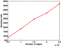
Figure 5: Speedup ratio vs. graph size.

V Related work

The $k$-core decomposition in networks has been extensively studied in the literature. In [22], Seidman introduces the concept of $k$-core for measuring the group cohesion in a network. The cohesion of the $k$-core increases as $k$ increases. Recently, the $k$-core decomposition in graph has been successfully used in many application domains, such as visualization of large complex networks [7, 9, 4, 3, 25], uncovering the topological structure of the Internet [10, 5, 2], analysis of the structure and function of the biological networks [17, 1, 23], studying percolation in random graph [14, 15], as well as identifying the influential spreader in complex network [18]. Below, we list some notable work on these applications.

In [7], Batagelj et al. propose to use $k$-core decomposition to visualize the large graph. Specifically, they first partition a large graph into smaller parts using the $k$-core decomposition and then visualize each smaller part by standard graph visualization tools. In [9], based on the $k$-core decomposition, Baur et al. present a method for drawing autonomous systems graph using 2.5D graph drawing. Their algorithm makes use of a spectral layout technique to place the nodes in the highest order core. Then, the algorithm uses an improved directed-forces method to place the nodes in each $k$ core according to the decreasing order. Alvarez-Hamelin et al. [4, 3] propose a visualization algorithm to uncover the hierarchical structure of the network using $k$-core decomposition. Their algorithm is based on the hierarchical property of $k$-core decomposition. More recently, Zhang and Parthasarathy [25] introduce a different notion, namely triangle $k$-core, to extract the clique-like structure and visualize the graph. Unlike the traditional $k$-core, the triangle $k$-core is the maximal subgraph that each edge of the subgraph is contained within at least $k$ triangles. They also propose a maintenance technique for triangle $k$-core. Since the triangle $k$-core is totally different from $k$-core, their maintenance technique cannot be applied in our problem. The $k$-core decomposition is also successfully used for analyzing and modeling the structure of the Internet [10, 5, 2]. For example, in [10], Carmi et al. study the problem of mapping the Internet using the method of $k$-core decomposition. In [5], Alvarez-Hamelin et al. investigate the hierarchies and self-similarity of the Internet using $k$-core decomposition. Besides the Internet, the $k$-core decomposition has also been applied to analyze the structure and function of the biological networks. In [17], Kitsak et al. propose a method based on the notion of $k$-core to find the molecular complexes in protein interaction networks. Altaf-Ul-Amin et al. [1] propose a technique for predicting the protein function based on $k$-core decomposition. In [23], Wuchty and Almaas apply the $k$-core decomposition to identify the layer structure of the protein interaction network. In addition, the $k$-core decomposition is recently used to identify the influential spreaders in complex network [18]. In [18], Kitsak et al. find that the nodes located in the high order core are more likely to be a influential spreader. Another line of research is to investigate the $k$-core percolation in a random graph [14, 15, 11]. These studies mainly focus on investigating the threshold phenomenon of the existence of a $k$-core based on some specific random graph models.

From an algorithmic point of view, Batagelj and Zaversnik propose an $O(n+m)$ algorithm for $k$-core decomposition in general graphs [8]. Their algorithm recursively deletes the node with the lowest degree and uses the bin-sort algorithm to maintain the order of the nodes. However, this algorithm needs to randomly access the graph, thus it could be inefficient for the disk-resident graphs. To overcome this problem, in [12], Cheng et al. propose an efficient $k$-core decomposition algorithm for the disk-resident graphs. Their algorithm works in a top-to-down manner that calculates the $k$-cores from higher order to lower order. To make the $k$-core decomposition more scalable, in [21], Montresor et al. propose a distributed algorithm for $k$-core decomposition by exploiting the locality property of $k$-core. All the above mentioned algorithms are focus on $k$-core decomposition in static graph except for [20]. For the dynamic graph, in [20], Miorandi and Pellegrini apply the $O(n+m)$ algorithm given in [8] to recompute the core number of the nodes when the graph is updated, which is clearly inefficient. In the present paper, we propose a more efficient core maintenance algorithm in dynamic graphs. Our algorithm are quite efficient, which is more than 100 times faster than the re-computation based algorithm.

VI Conclusions

In this paper, we propose an efficient algorithm for maintaining the core number of nodes in dynamic graphs. For a node $u$, we define a notion of induced core subgraph $G_{u}$, which contains the nodes that are reachable from $u$ and have the same core number as $u$. Given a graph $G$ and an edge $(u,v)$, we find that only the core number of nodes in $G_{u}$ or $G_{v}$ or $G_{u\cup v}$ may need to be updated after inserting/deleing the edge $(u,v)$. Based on this, first, we introduce a coloring algorithm to identify all of these nodes. Second, we devise a recoloring algorithm to determine the nodes whose core numbers definitely need to be updated. Finally, we update the core number of such nodes by a linear algorithm. In addition, we develop two pruning strategies, namely $X$-pruning and $Y$-pruning, to further accelerate the algorithm. We evaluate our algorithm over 15 real-world and 5 large synthetic datasets. The results demonstrate the efficiency of our algorithm.

References

- [1] M. Altaf-Ul-Amin, K. Nishikata, T. Koma, T. Miyasato, Y. Shinbo, M. Arifuzzaman, C. Wada, M. Maeda, T. Oshima, H. Mori, and S. Kanaya. Prediction of protein functions based on k-cores of protein-protein interaction networks and amino acid sequences. Genome Informatics, 14, 2003.
- [2] J. I. Alvarez-Hamelin, M. G. Beiró, and J. R. Busch. Understanding edge connectivity in the internet through core decomposition. Internet Mathematics, 7(1):45–66, 2011.
- [3] J. I. Alvarez-Hamelin, L. Dall’Asta, A. Barrat, and A. Vespignani. k-core decomposition: a tool for the visualization of large scale networks. CoRR, abs/cs/0504107, 2005.
- [4] J. I. Alvarez-Hamelin, L. Dall’Asta, A. Barrat, and A. Vespignani. Large scale networks fingerprinting and visualization using the k-core decomposition. In NIPS, 2005.
- [5] J. I. Alvarez-Hamelin, L. Dall’Asta, A. Barrat, and A. Vespignani. K-core decomposition of internet graphs: hierarchies, self-similarity and measurement biases. NHM, 3(2):371–393, 2008.
- [6] A.-L. Barabasi and R. Albert. Emergence of scaling in random networks. science, 1999.
- [7] V. Batagelj, A. Mrvar, and M. Zaversnik. Partitioning approach to visualization of large graphs. In Graph Drawing, pages 90–97, 1999.
- [8] V. Batagelj and M. Zaversnik. An o(m) algorithm for cores decomposition of networks. CoRR, cs.DS/0310049, 2003.
- [9] M. Baur, U. Brandes, M. Gaertler, and D. Wagner. Drawing the as graph in 2.5 dimensions. In Graph Drawing, pages 43–48, 2004.
- [10] S. Carmi, S. Havlin, S. Kirkpatrick, Y. Shavitt, and E. Shir. A model of internet topology using k-shell decomposition. PNAS, 104(27):11150–11154, 2007.
- [11] D. Cellai, A. Lawlor, K. A. Dawson, and J. P. Gleeson. Tricritical point in heterogeneous k-core percolation. Physical review letters, 107.
- [12] J. Cheng, Y. Ke, S. Chu, and M. T. Özsu. Efficient core decomposition in massive networks. In ICDE, 2011.
- [13] J. Cohen. Trusses: Cohesive subgraphs for social network analysis. Technique report, 2005.
- [14] S. N. Dorogovtsev, A. V. Goltsev, and J. F. F. Mendes. k-core organization of complex networks. Phys. Rev. Lett., 96(4), 2006.
- [15] A. V. Goltsev, S. N. Dorogovtsev, and J. F. F. Mendes. k-core (bootstrap) percolation on complex networks: Critical phenomena and nonlocal effects. CoRR, abs/cond-mat/0602611, 2006.
- [16] R. A. Hanneman and M. Riddle. Introduction to social network methods. Online book, 2005.
- [17] M. Kitsak, L. K. Gallos, S. Havlin, F. Liljeros, L. Muchnik, H. E. Stanley, and H. A. Makse. An automated method for finding molecular complexes in large protein interaction networks. BMC Bioinformatics, 4, 2003.
- [18] M. Kitsak, L. K. Gallos, S. Havlin, F. Liljeros, L. Muchnik, H. E. Stanley, and H. A. Makse. Identification of influential spreaders in complex networks. Nature Physics, 6:888–893, 2010.
- [19] J. Leskovec. Standford network analysis project. 2010.
- [20] D. Miorandi and F. D. Pellegrini. K-shell decomposition for dynamic complex networks. In WiOpt, 2010.
- [21] A. Montresor, F. D. Pellegrini, and D. Miorandi. Distributed k-core decomposition. In PODC, pages 207–208, 2011.
- [22] S. B. Seidman. Network structure and minimum degree. Social networks, 5(3):269–287, 1983.
- [23] S. Wuchty and E. Almaas. Peeling the yeast protein network. Proteomics, 5, 2005.
- [24] R. Zafarani and H. Liu. Social computing data repository at ASU, 2009.
- [25] Y. Zhang and S. Parthasarathy. Extracting analyzing and visualizing triangle k-core motifs within networks. In ICDE, 2012.