Tessellating the cosmological dark-matter sheet: origami creases in the universe and ways to find them

Abstract

Tessellations are valuable both conceptually and for analysis in the study of the large-scale structure of the universe. They provide a conceptual model for the ‘cosmic web,’ and are of great use to analyze cosmological data. Here we describe tessellations in another set of coordinates, of the initially flat sheet of dark matter that gravity folds up in rough analogy to origami. The folds that develop are called caustics, and they tessellate space into stream regions. Tessellations of the dark-matter sheet are also useful in simulation analysis, for instance for density measurement, and to identify structures where streams overlap.

1 Introduction: the cosmological dark-matter sheet

In Einstein’s theory of general relativity, gravity comes about through the distortion that matter and energy produce in the four-dimensional manifold of spacetime. Gravity also causes another manifold that pervades spacetime to distort and fold: the sheet of dark matter.

Just after the big bang, the matter was almost uniformly distributed, i.e. the density varied very little from point to point in space. These tiny density fluctuations are thought to be random quantum fluctuations that were ‘inflated’ in the first instants to macroscopic size.

It is useful to think of the matter occupying vertices of a regular mesh, and to represent the density fluctuations as small distortions of this mesh. Where there is a bit more matter than average, the mesh has contracted, and where there is less matter than average, the mesh has expanded.

As particles move around in three-dimensional space, they occupy worldlines in four-dimensional spacetime. It is also useful to think of particle trajectories in yet another, six-dimensional ‘phase space’ of position and velocity. Each particle in the universe can be plotted in this 6D phase space, three of the dimensions given by its spatial position, and three by its velocity.

In phase space, the primordial state of the universe was well characterized by particles separated from each other in position dimensions, but with little separation in velocity (all velocities, after subtracting out the universe’s expansion, were nearly zero). In this sense, the matter sheet was ‘flat.’ The coordinates of a particle within the initial, flat sheet is called its Lagrangian position; this remains constant for a given particle for all time. The usual position of a particle as it moves around in space is called its Eulerian position.

As time passes, the largest effect on the matter sheet is stretching from the expansion of the universe, which generally increases the physical spatial separation of particles. As is usually done in cosmology, however, we use comoving coordinates, i.e. we divide out the expansion. The comoving coordinates of particles at rest with respect to the expansion of the universe do not change.

Gravity also amplifies the small distortions in the matter-sheet sheet, increasing velocities. In fact, the dark-matter sheet has special physical significance in general relativity: it is the set of observers (dark-matter particles) that have been freely falling in gravity since the big bang. This follows from the (astronomical) definition of dark matter as matter that interacts only through gravity.

The growth of structure in the universe is a balance between gravity pulling matter together and the expansion of the universe damping such motions, as seen in comoving coordinates. Nevertheless, in ‘overdense’ regions where the sheet has contracted, more matter accumulates, so the sheet contracts further. Likewise, underdense regions repel matter, expanding the sheet to form a void.

In overdense regions, the sheet eventually bunches together and folds. Gas (normal matter) collects in these regions, and forms galaxies. When two gas streams encounter each other, they collide and shock, to a good approximation forcing a unique gas velocity at each point.

The dominant form of matter in the universe, dark matter, on the other hand, only interacts gravitationally. Two dark-matter particles encountering each other at the same position do not collide, i.e. do not change their trajectories. (In many models, dark matter can very rarely collide, but here we neglect this possibility.) Often a single point of Eulerian space can have dark matter flowing with many discrete velocities. Thus (given the spatial continuity of the mapping from initial to final positions), the dark-matter sheet has folded up, if considered in 6D phase space. Since particles cannot have the same positions and velocities without also being initially coincident, the mesh cannot intersect itself.

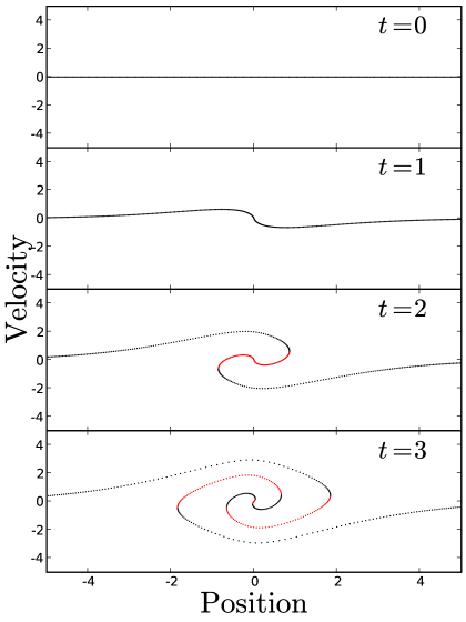
Figure 1: A schematic phase-space spiral that corresponds to the collapse of a ‘halo’ in a one-dimensional universe. Patches oriented forwards in position space (i.e. projecting down to the $x$-axis) are colored black, while patches oriented backwards are red. These two possibilities make the set of streams (contiguous patches with the same orientation) two-colorable. All one-dimensional sets of contiguous regions are two-colorable, but when we go to two and three dimensions, this property becomes quite special.

A schematic example of halo collapse in a one-dimensional universe (with therefore a two-dimensional position-velocity phase space) is shown in Fig. 1. Particles start out equally separated, but are drawn into the center, their Lagrangian string winding up into a spiral. The quasi-circularity of the spiral comes from particles oscillating back and forth about the center of the potential. Different orientations of the initially flat string of dark-matter particles are colored black (forward) and red (backward). Contiguous regions on the string that are oriented the same way are called streams. The boundaries between streams, folds in the string when projected down to the $x$-axis, are called caustics. At caustics, in the limit of infinitesimal particles and infinite spatial resolution, the densities become infinite. Thus they may greatly enhance the chances of observing dark matter, which may collide observably in very dense environments (Hogan,, 2001; Natarajan & Sikivie,, 2008; Vogelsberger & White,, 2011).

The folding in this figure suggests an analogy to origami: indeed, cosmic structure is built out of origami-like folds, although there are some differences in detail. The rest of this contribution is organized as follows. First, in Sec. 2, we describe some mathematical propeties of paper origami, and how to understand origami crease patterns in terms of tessellations. In Sec. 3, we explain the analogy between paper and cosmological origami in detail. Then, in Sec. 4, we give some properties of the structures gravity builds from origami-folding up the dark-matter sheet. In Sec. 5, we describe how various tessellations of the dark-matter sheet in Lagrangian space can be used to analyze and extract useful information from cosmological simulations.

2 Origami mathematics

There has been much mathematical work in origami, most of it recent in the ancient history of the art form Row, (1966); Martin, (1998); Lang, (2003); Hull, (2006). ‘Flat origami’ is the class of origami most easily relatable to large-scale structure. In flat origami, folding of a two-dimensional sheet is allowed in three dimensions, but the result is restricted to lie flat in a plane, i.e. it could be squashed between pages in a book without acquiring any new creases. The class of flat-foldable origami is quite large, for example encompassing the paper crane, similar to the model shown in Fig. 2.

There are several theorems that have been proven about flat origami (Hull,, 1994, 2002). One is the two-colorability of polygons outlined by origami crease lines, as shown in Fig. 1 in one dimension. Two colors suffice to color them so that no adjacent polygons share the same color.

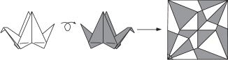
Figure 2: Two-coloring of the polygons outlined by creases in an origami ‘traditional Japanese flapping bird’ (similar to a crane). Polygons facing ‘up’ (out of the page in the leftmost diagram, with the head facing to the left) are colored white, while polygons facing ‘down’ (into the page in the leftmost diagram) are painted gray. The crane has been unfolded for the rightmost diagram. Creases are shown as lines here; the polygons outlined by them may be colored with only two colors, such that polygons straddling creases never have the same color. Figure from Hull, (2006), courtesy Tom Hull.

To see why two colors suffice, consider the bird in Fig. 2. Both sides of it are shown, along with its appearance when unfolded. Each polygon is colored white or gray according to whether the polygon is facing ‘up,’ i.e. with the same orientation as it did initially, or ‘down,’ if it has been flipped over. This uniquely colors each polygon, and each crease does indeed divide ‘up’ from ‘down’ polygons. According to the four-color theorem (e.g. Wilson, (2002)), a general set of planar regions is colorable by four colors. So, the ability to produce a flat-foldable origami design from a crease pattern reduces the so-called chromatic number (the number of colors necessary such that neighboring regions are not colored the same) from four to two.

A work of flat origami can be thought of as a function (specifically, a continuous piecewise isometry) mapping the unit square (the unfolded sheet at right in Fig. 2) into the plane. Each crease produces a reflection, reversing the direction of the vector on the paper perpendicular to the crease. The function is defined on each polygon by a sequence of these reflections. The color in each polygon corresponds to its parity, i.e. depending on whether the number of reflections used to define the function on that polygon is odd or even. The parity can also be measured locally with the determinant of the matrix defining the function on the polygon; we will also use this latter definition in the cosmological case below.

Besides two-colorability, there are other properties that flat-foldable crease patterns have. For example, Maekawa’s theorem states that in a flat-foldable crease pattern, the numbers of ‘mountain’ and ‘valley’ creases around a vertex differ by two. (A mountain crease becomes folded to form an upward-pointing ridge; a valley crease is folded in the opposite way.) Maekawa’s theorem is likely to be applicable to a stretchable 3D cosmological sheet, as well, in a more complicated form, but we have not investigated this possibility.

Even for paper origami, a difficult problem is to test that an arbitrary crease-pattern is physically flat-foldable without the paper intersecting any folds; this is an NP-complete problem (Bern & Hayes,, 1996). There are further results that, for instance, describe the angles around vertices, but they depend on the non-stretchability of the origami sheet, making them inapplicable to the cosmological case.

3 Origami large-scale structure

Moving from paper origami to cosmological structure formation introduces a few changes. The manifold (sheet) has three instead of two dimensions. It folds in six dimensions (three position, and three velocity) instead of three. The sheet also stretches inhomogeneously, stretching more in voids than in dense regions. In dense regions, it can also stretch violently in the velocity dimensions.

In spite of these differences, it is still possible to approximate two-dimensional large-scale structures with origami designs. Fig. 3 shows a work of flat origami that bears some resemblance to the cosmic web of filaments and clusters in cosmology. The ‘voids’ are Voronoi cells generated from black pencil-marks on the paper. Voronoi models of large-scale structure are good heuristic models of cosmological structure formation Icke & van de Weygaert, (1987); Kofman et al., (1990); Hidding et al., (2012). The present figure corresponds most closely to a Zel’dovich-approximation evolution of particle displacements, in which structures fold up when expanding voids collide, but overshoot and do not undergo realistic further collapse.

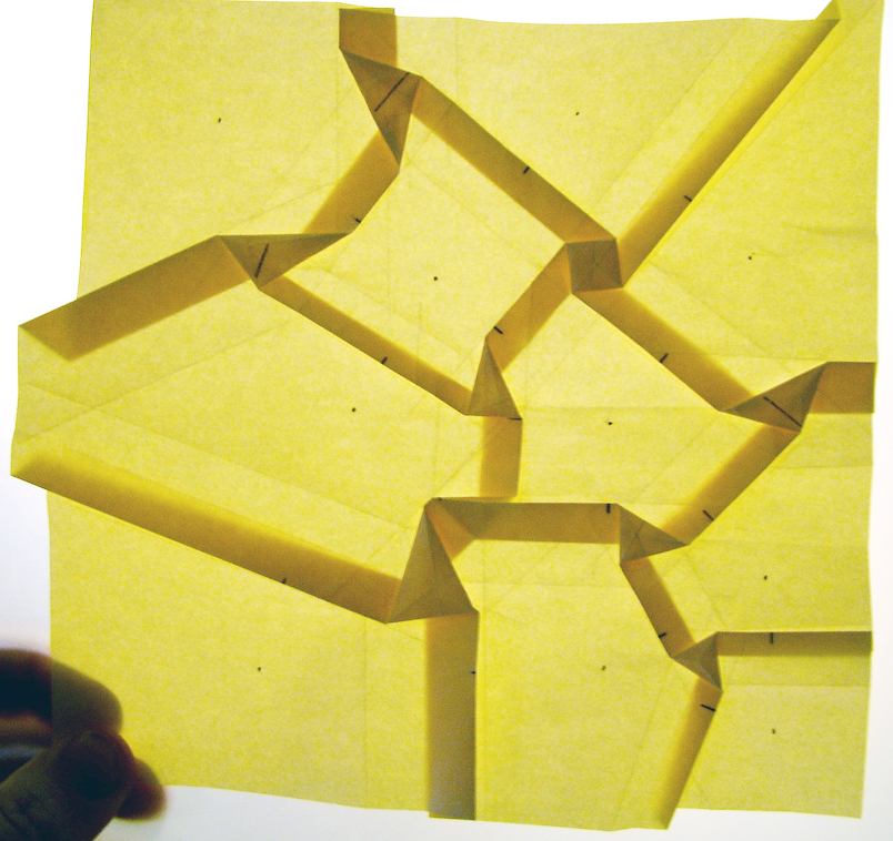
Figure 3: A Voronoi origami tessellation that resembles cosmological voids, filaments and haloes in a two-dimensional universe. If the work were unfolded, the polygons outlined by creases would be two-colorable according to which way the polygon is facing. E.g. ‘voids’ and the topmost polygons in ‘haloes’ could be colored black, and the paper turned upside down within the ‘filaments’ could be colored white. Design and photo by Eric Gjerde (http://www.origamitessellations.com/), used with permission.

Fig. 4 shows two crease patterns: one that folds up into a single schematic ‘galaxy,’ and one that folds up into a hexagonal void surrounded by six galaxies. They have proven useful at public-outreach events, and are available at http://skysrv.pha.jhu.edu/~neyrinck/origalaxies.html. These designs are based on elements of Eric Gjerde’s ‘Tiled Hexagons’ pattern, in his Origami Tessellations book Gjerde, (2008), which contains several other interesting origami tessellations.

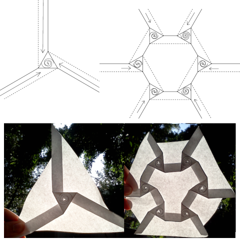
Figure 4: Top, crease patterns that fold up into schematic ‘galaxies’ surrounded by filaments, at bottom. In the crease patterns, solid lines give mountain folds, folding to form a ridge, and dashed lines give valley folds. The arrows indicate the direction of matter flow within the folded-up filaments.

These figures are interesting pedagogically, but also suggest a reason why filaments are so common in the universe. Here, galaxies, or knots, cannot form without associated filaments. This requirement comes from the non-stretchability of origami paper (a property which the dark-matter sheet lacks), but it still suggests a strong tendency for filaments to form along with galaxies. It also suggests a reason why galaxies tend to accrete much angular momentum: it seems to be easier to fold a galaxy when the filament has a nonzero impact parameter with respect to the center of the galaxy. When the accreting matter arrives in the galaxy, it then torques it up. These are not proofs, but interesting suggestions.

Moving toward more mathematical rigor, we now consider local parities of patches on the cosmological sheet. The parity may still be defined in the same way as in flat origami, and it may have only one of two values (positive or negative). The parity at a particle is measurable from how the particles initially adjacent to it have distorted around it. Mathematically, the parity is the sign of the determinant of the deformation tensor that takes initial to final coordinates; see for example White & Vogelsberger, (2009); Neyrinck, (2012) for details.

3.1 Streams and caustics in Lagrangian space

The dark-matter sheet folds up in Eulerian space in an overwhelmingly rich way, visually corresponding somewhat to rococo art. Beautiful figures of the structure that develops can be seen in Vogelsberger & White, (2011), for example.

We defined caustics and streams for a 1D universe around Fig. 1, and use the same definitions in a 3D universe. A stream is a contiguous three-dimensional region with the same orientation, or parity. A caustic is a two-dimensional surface separating streams from each other. Defined this way, a caustic indeed corresponds to a fold, since the parity swaps if one moves across it.

By definition, then, Lagrangian space (the dark-matter sheet) is tessellated by streams that are outlined by caustics. In addition, the streams are two-colorable, just as in paper origami. This is because the parity may take only two values, and changes as one crosses a caustic along the sheet.

Two-colorability may seem hopelessly academic, and indeed it does not have obvious observational consequences. But in fact it greatly restricts the arrangement of streams on the unfolded dark-matter sheet. A tessellation in greater than two dimensions has in principle no bound on its chromatic number (the number of colors required). In relation to the famous four-color theorem (four colors suffice to color any planar arrangement of regions), Guthrie Guthrie, (1880) discussed the impossibility of restricting the chromatic number of an arrangement of solid regions in three dimensions. He constructed a set of arbitrarily many long sticks, each of which touches all others. Such an arrangement is possible, for example, if each stick is slightly rotated from its neighbor. Flexible sticks are especially capable of touching all the others; imagine a bowl of arbitrarily long spaghetti noodles. In this case, the chromatic number is bounded only by the number of sticks.

In graph theory, a two-colorable graph is called bipartite. Using the graph-theory terms of ‘vertices’ that are linked by ‘edges,’ the vertices of the cosmological bipartite graph are the three-dimensional stream regions, and the edges are the caustic surfaces between them.

At least one whole book is devoted to the subject of bipartite graphs (Asratian et al.,, 1998); here we list a few of their properties, translating into cosmological terms. First, there is no path (stepping from stream to stream through caustics) starting and ending at the same stream that consists of an odd number of steps. Another result, König’s Minimax Theorem, pertains to the necessity of caustics to form streams. It states that the minimum number of streams needed to touch all caustics with streams equals the maximum possible number of caustics involved in a matching between streams of opposite parity. A ‘matching’ is a set of caustics linking pairs of streams, such that no stream is touched by more than one caustic. Considering the dual graph, in which streams and caustics swap roles, König has another result. His Coloring Theorem for bipartite graphs applies to the dual graph of caustics joined by streams: the chromatic number for the dual graph equals the maximum number of caustics around a single stream. If the graph of streams joined by caustics were not bipartite, the dual graph would generally have a larger chromatic number than the maximum number of caustics around a single stream.

We close this section with a technical caveat about this stream-caustic definition. In principle, the stretchable cosmological sheet can fold in a way that is impossible for paper origami. Unlike paper folds, cosmological caustics can form through spherical or cylindrical collapse, not just planar collapse. Spherical collapse reverses parity just as in planar collapse, but cylindrical collapse does not; it simply produces a 180^∘ rotation in the two axes perpendicular to the cylinder. However, in a physically realistic situation, the probability that more than one axis will collapse exactly simultaneously is zero, so we adopt the view that caustics always form one-at-a-time, if viewed at sufficiently high resolution.

3.2 Simulation measurements

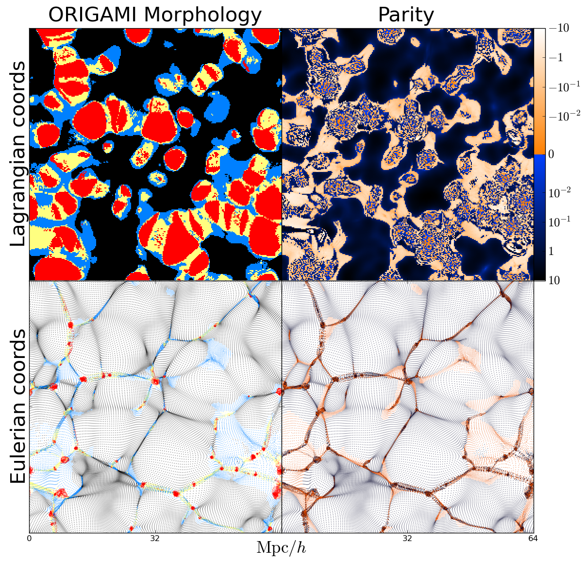
Figure 5: The folding of a cosmological sheet (top, unfolded; bottom, folded). Quantities were measured from a 2D sheet of particles from a 3D $\Lambda$CDM $N$-body simulation. The $256^{2}$ particles share the same $z$-coordinate in the initial-conditions lattice, where $z$ points out of the page. Before running the simulation, the initial conditions were smoothed with a 1 $h^{-1}$ Mpc Gaussian window, to inhibit small-scale structure formation. Top panels use Lagrangian coordinates, in which each particle is a square pixel in a 256²-pixel image. In the bottom panels, particles are shown in their actual present-epoch Eulerian $(x,y)$ coordinates, projecting out the $z$ coordinate (in which the slice does have some extent). In left-hand panels, void, wall, filament and halo origami morphologies are shown in black, blue, yellow and red, respectively. In right-hand panels, particles are colored according to $J$, i.e. the volume of their fluid element times its parity. Black/blue particles have right-handed parity (as in the initial conditions), and white/orange particles have swapped, left-handed parity.

Fig. 5 shows the folding up of a 2D cosmological sheet of particles from a $\Lambda$CDM (the current, observationally successful model of cosmology) 3D gravitational simulation, with its initial small-scale fluctuations dampened for clarity. In the top panels, pixels represent particles in the square grid of Lagrangian coordinates; in origami terms, this is the flat sheet before folding. The bottom panels show particles in Eulerian coordinates.

The ‘morphology’ of the left panels describes whether they are void, filament, sheet, or halo particles. This morphology is measured using the origami Falck et al., (2012) algorithm discussed above (not to be confused with the origami analogy itself).

In the right panels, particles are colored primarily by parity (white/orange or black/blue). Particles which have been flipped by caustics an even number of times (including zero) and have the original, right-handed orientation are black/blue; particles that have been flipped an odd number of times and have left-handed orientation are white/orange. In the finer color gradation (along the white/orange or black/blue spectra), the upper-right panel additionally shows the magnitude of the volume each particle occupies on the dark-matter sheet (inversely proportional to its density). Note that the magnitude is quite small in the cores of halo regions, because mass elements shrink considerably in high-density halo regions.

There is some agreement between outer caustics identified by origami morphology (the boundaries between black and non-black regions) and as measured by parity (the outermost boundaries between dark blue and light orange regions), but the agreement is not perfect. See Neyrinck, (2012) for further discussion and details.

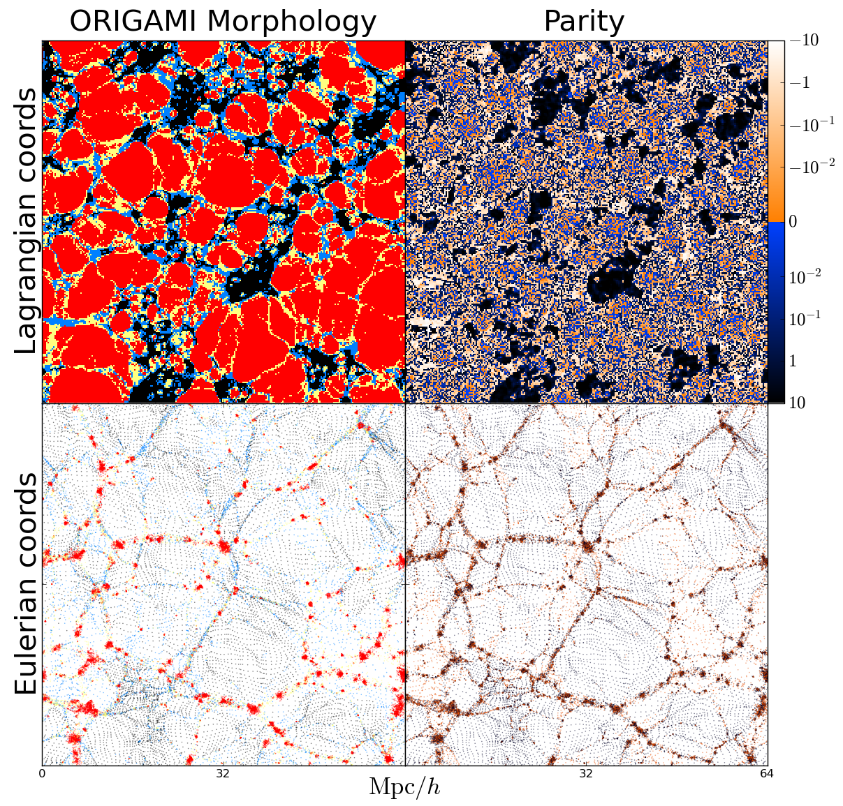
Figure 6: Same as Fig. 5, except measured from a simulation with full initial power, i.e. unsmoothed initial conditions.

Fig. 6 is the same figure as Fig. 5, except that the simulation was run without smoothing the initial conditions, causing the true amount of small-scale structure to appear. This structure in Fig. 6 makes the parity map (the upper-right panel) much more cluttered. There are many visible extended streams (patches of identical parity), especially those that correspond to large voids, but much of the plot looks essentially random. Note also here that the Lagrangian patches that correspond to voids are much smaller than in the previous figure, indicating that the dark-matter sheet has stretched more. Given the near-randomness of the parity deep within haloes, it seems that particles here have crossed many, many caustics. We caution, however, that some of this apparent randomness could be ‘noise’ from finite resolution.

4 Properties of structures built from folds in the dark-matter sheet

Now we turn our attention to the structures built up by caustics in the dark-matter sheet. Zel’dovich Zel’dovich, (1970) predicted the formation of caustics at the stage when the evolution of the density field reaches non-linearity. Fig. 7 illustrates the beginning of the structure formation when a few very thin concentrations of mass emerged. It is worth noting that in order to avoid blocking the view only a relatively small sphere cut from the large volume is shown. The surfaces seen in the figure are the caustic surfaces where density is formally infinite. A very thin layer of highly compressed matter between two caustics form the first nonlinear structures which Zel’dovich called pancakes. Initially each pancake consists of three streams of mass moving with different velocities through each other, as illustrated in Fig. 7. As time passes, pancakes grow in size, merge with other pancakes and develop an intricate structure shown in Fig. 8. The number of streams in pancakes rapidly grows, and in addition, filaments and compact halos emerge. If the flow has no curl – a condition which holds to a good approximation except in highly nonlinear regions – Arnold rigorously proved that only six generic types of singularities exist. According to Arnold’s ADE classification, these are $A_{2}$ (surfaces shown in Figures 7 and 8) and $A_{3}$ (lines seen as the contours of pancakes in those figures). The remaining four types occur in isolated points: $A_{4}$ and $D_{4}$, that persist for some finite length of time, and $A_{5}$ and $D_{5}$, that exist only instantaneously. There are also subclasses in some of these classes but the details are not important for the current discussion.

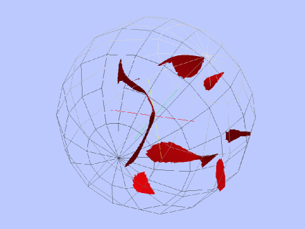
Figure 7: A few isolated pancakes bounded by caustics are shown at the early stage of the evolution described by Eq. (1).

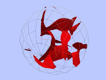
Figure 8: Pancakes have grown in size and some of them merged into a large connected structure.

In the Zel’dovich approximation Zel’dovich, (1970); Arnold et al., (1982); Shandarin & Zeldovich, (1989) the singularities can be found directly from the initial velocity field ${\mbox{\boldmath$v$}}({\mbox{\boldmath$q$}})=-\nabla\Phi({\mbox{\boldmath$q$}})$ that completely determines the evolution via a simple map

$$x_{i}(q,t)=q_{i}+Dv_{i},~{}~{}~{}v_{i}\equiv{d\,x_{i}\over d\,D}=v_{i}(q).$$ (1)

Here we use so-called comoving coordinates, that exclude the uniform expansion of the universe. The function $D=D(t)$ monotonically increases with physical time, and thus can be used as a time coordinate. The coordinates $x_{i}$ and $q_{i}$ are the Eulerian and Lagrangian coordinates of the fluid particles. The volume of a fluid element can be found from the continuity equation and can be conveniently expressed in terms of the eigenvalues $\lambda_{1}(q),\,\lambda_{2}(q),\,\lambda_{3}(q)$ of the deformation tensor $d_{ik}\equiv-\partial v_{i}/\partial q_{k}$:

$$V(q,t)=V_{0}(1-D\lambda_{1})(1-D\lambda_{2})(1-D\lambda_{3}).$$ (2)

The volume collapses to zero when one factor in parentheses in the above equation vanishes. At this instant of time the fluid particle is squashed into one of two dimensional surface elements comprising the caustic surface and then expands with different parity. If one assumes that three eigenvalues at each point are ordered [$\lambda_{1}(q)\geq\lambda_{2}(q)$ and $\lambda_{2}(q)\geq\lambda_{3}(q)$] then the first pancakes arise around maxima of $\lambda_{1}(q)$.

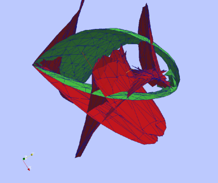
Figure 9: Caustics related to two eigenvalues are shown by different colors. The nice smooth edges of caustics are due to cutting by an enclosing sphere (not shown).

For a while only the caustics of $A$ types, related to $\lambda_{1}$, occur. Then $A$-singularities related to $\lambda_{2}$ and $\lambda_{3}$ as well as $D$-singularities related to points where $\lambda_{1}(q)=\lambda_{2}(q)$ or $\lambda_{2}(q)=\lambda_{3}(q)$ arise. It is worth remembering that the points where all three eigenvalues would have the same value do not exist in a generic field. Figure 9 shows two types of caustics (red and green) related to two eigenvalues in a small sphere (not shown).

Even a relatively simple evolution described by the Zel’dovich approximation results in a very complex structure of caustics characterized by numerous intricate crossings. Unfortunately the Zel’dovich approximation can be used for a qualitative or crude quantitative analysis of the structure in the universe only at early nonlinear stages, although straightforward modifications can improve some aspects of the approximation Coles et al., (1993); Sahni & Coles, (1995); Neyrinck, (2012). The more realistic picture emerging from cosmological N-body simulations shows that the complexity of the structure grows with increasing rate in the concentrations of mass, in particular in halos Vogelsberger & White, (2011).

The presentation of the N-body results in the form of particle plots is a far more popular in cosmological literature than other types of illustrations. Unfortunately the pictures of the particle distributions fail to reveal caustics in N-body simulations except for the most massive caustics in the simulations of a single halo with billions of particles Vogelsberger & White, (2011).

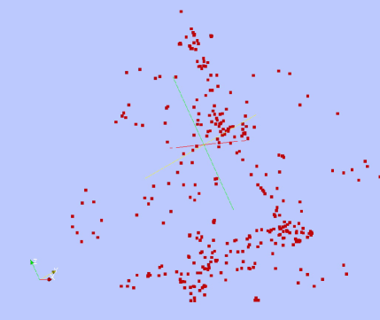
Figure 10: A particle representation of the caustics.

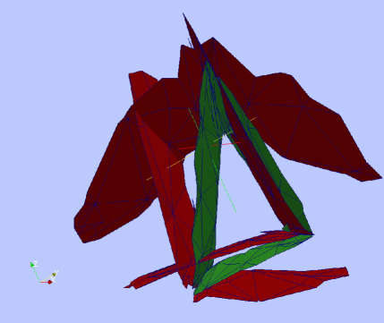
Figure 11: Tessellation representation of the same structure as shown by the particles.

Probing the caustic structure in gravitationally bound halos is a difficult problem which has not been properly addressed until rather recently. White & Vogelsberger White & Vogelsberger, (2009) proposed a method to detect caustic crossings in a running simulation, watching the deformation of small mass elements around particles at each timestep. Very recently, Shandarin et al. [2012] and Abel et al. [2011] more explicitly tracked the dynamics of the phase-space sheet, crucially using a tessellation within it. This allows greater progress to be made from a single snapshot. Although the methods differ in some details, the basic idea was the same in both studies. The advantage of a tessellation technique over a particle representation is illustrated in Figures 10 and 11. Figure 10 shows the particles lying on two caustic surfaces related to $\lambda_{1}$ and $\lambda_{2}$ . Figure 11 using exactly the same information as the dot plot shows two families of caustics in red and green. Now the particles are treated as the vertices of the tessellation of the phase space sheet. In the next section we briefly explain the method.

5 Tessellations within the dark-matter sheet for studying caustics

In this section, we explore tessellations that are useful for finding and analyzing two-dimensional creases in three-dimensional space.

First, though, we briefly review some techniques that work purely in Eulerian space to detect structures. These have the clear advantage that they can be applied to observations in principle, in which the initial conditions are not known. Some of these Eulerian techniques are entirely local, depending on the local arrangement of mass Hahn et al., (2007); Aragón-Calvo et al., (2007); Sousbie et al., (2008); Sousbie, (2011). Another approach is global, defining voids to tessellate space. For instance, voids can be defined as density depressions outlined by a watershed transform (Platen et al.,, 2007; Neyrinck,, 2008). In this framework, walls, filaments, and haloes are defined according to where voids meet each other, and the dimensionality of borders separating them (Aragón-Calvo et al.,, 2010). Another dynamical algorithm for void-finding Lavaux & Wandelt, (2010) estimates orbits of particles in the final conditions, designed to detect structures in the primordial density field.

The first step in the Lagrangian-tessellation algorithm for studying caustics is the ‘triangulation’ of Lagrangian space itself. The uniform cubic mesh often used for generating initial positions and velocities for the N-body simulations is triangulated by subdividing each cubic voxel of the mesh into five tetrahedra. The vertices of these tetrahedra are the particles being tracked through the simulation, which can be alternatively thought of as vertices of a mesh covering the phase-space sheet. The tetrahedra represent the fluid elements that continuously fill the space. The mass particles moving in the course of the gravitational evolution deform the tetrahedra but do not fracture the continuity of the three-dimensional phase-space sheet. The tetrahedra change their parity every time they experience collapse in a two-dimensional triangle. Keeping the initial order of the vertices in each tetrahedron, one can identify the change of parity by the change of the sign in the volume of the tetrahedron as computed with a determinant.

The next step is to select the triangle faces shared by two neighboring tetrahedra with opposite parities. This completes the triangulation of the caustic surfaces at every time step. Figs. 7 and 8 show the evolution of the structure described by the Zel’dovich approximation. In this first-order theory, by Eq. (2), the parity of a fluid element can be changed at most three times. Given initial Gaussianity (which holds to a good approximation), one can easily find the statistics of parity evolution that is determined by the probability density function of three eigenvalues, $\lambda_{1},\,\lambda_{2},\,\lambda_{3}$. For instance, no more than about 92% of all fluid particles may experience one parity transition since in about 8% of the initial volume $\lambda_{1}$ is negative Doroshkevich, (1970). In the real world as well as in cosmological N-body simulations the number of parity changes is enormous.

Although the caustics are the boundaries between the regions with different number of streams there is no direct general relation between the number of streams and number of parity transitions due to nonlocal character of structure evolution described by mapping. For example, the interior part of the red cusp in Fig. 9 above the green caustic contains a different number of streams than the interior part lying below the green caustic. The particles lying on the crossing line of two caustics came from very different parts of Lagrangian space and their paths could be extremely weakly related.

These new numerical techniques allow a deeper insight into the complex nonlinear evolution of the large scale structure in the universe. An example of a useful outcome of the studies of caustics is a unique definition of physical voids as the regions of one-stream flows. An N-body simulation of the ’standard’ $\Lambda$CDM model showed that the total volume occupied by physical voids is about 93% of the total volume Shandarin et al., (2012).

Such tetrahedra also allow density estimates within the dark-matter mesh (Abel et al.,, 2011). The densities within each stream can then be added up to a density estimator in many ways more robust than Eulerian density estimates that ignore the initial arrangement of particles. The most common density estimates in cosmology are Eulerian, volume-weighted density estimates, for example counting the number of particles in each cell of a cubic grid. There are also mass-weighted density estimates, returning the density separately at each particle, for example using a Voronoi or Delaunay tessellation Schaap & van de Weygaert, (2000); Neyrinck et al., (2005); van de Weygaert & Schaap, (2009). These are usefully parameter-free and adaptive, but a truly Lagrangian density estimate (Abel et al.,, 2011) has the potentioal to be even more physically meaningful, defining the density at each position as a sum over Lagrangian streams. This would have minimal dependence on particle discreteness, and could prove quite useful to implement within $N$-body simulations. Although particle discreteness seems not to be a major issue usually, in some circumstances (such as warm-dark-matter simulations, where small-scale clustering is suppressed), artificial structures appear from particle discreteness (Wang & White,, 2007). In such cases, this truly Lagrangian density estimate could be essential for accuracy.

Tracking the parity as in these Lagrangian-tessellation methods allows collapsed structures to be detected, but does not immediately give their morphology (i.e. whether they are pancakes, filaments or haloes). Keeping track of the axes along which particles cross each other gives this extra information Falck et al., (2012), in an algorithm called origami. In the one-dimensional halo of Fig. 1, a natural place to put the boundary of the structure is at the transition between where one and three streams overlap when projected to the $x$ axis. In three dimensions, structures are classified according to how many perpendicular axes particles within them have been crossed along by other particles. Particles in voids, walls, filaments and haloes have been crossed along 0, 1, 2, and 3 perpendicular directions. This is a conveniently parameter-free, objective, geometrical, and dynamical identification of structures and placement of their boundaries. However, this simple particle-crossing criterion does not distinguish substructures from larger structures. Such subhaloes, coils in six-dimensional phase space, likely require a more sophisticated algorithm to detect.

6 Conclusion

A natural tessellation of the final, observed matter and galaxy distribution (known as Eulerian space) is into voids, as explored elsewhere in this volume. Tessellations in Eulerian space are also of great use for measuring quantities such as densities and velocities adaptively. In this contribution, we described tessellations of the initial dark-matter sheet (known as Lagrangian space). The natural tessellation in this case is like an origami crease pattern, dividing the sheet into streams bordered by folds, or caustics. Also as in the Eulerian case, tessellations are useful for analysis, for detecting stream-crossings and estimating densities natively within the dark-matter sheet.

References

- Abel et al., (2011) Abel, T., O. Hahn, & R. Kaehler 2011. Tracing the Dark Matter Sheet in Phase Space. MNRAS, submitted, arXiv:1111.3944.
- Aragón-Calvo et al., (2007) Aragón-Calvo, M. A., B. J. T. Jones, R. van de Weygaert, & J. M. van der Hulst 2007. The multiscale morphology filter: identifying and extracting spatial patterns in the galaxy distribution. A&A, 474:315–338.
- Aragón-Calvo et al., (2010) Aragón-Calvo, M. A., E. Platen, R. van de Weygaert, & A. S. Szalay 2010. The Spine of the Cosmic Web. ApJ, 723:364–382.
- Arnold et al., (1982) Arnold, V. I., S. F. Shandarin, & I. B. Zeldovich 1982. The large scale structure of the universe. I - General properties One- and two-dimensional models. Geophysical and Astrophysical Fluid Dynamics, 20:111–130.
- Asratian et al., (1998) Asratian, A.S., T.M.J. Denley, & R. Häggkvist 1998. Bipartite graphs and their applications. Cambridge tracts in mathematics. Cambridge University Press.
- Bern & Hayes, (1996) Bern, Marshall, & Barry Hayes 1996. The Complexity of Flat Origami (Extended Abstract). In Proceedings of the 7th Annual ACM-SIAM Symposium on Discrete Algorithms, pages 175–183.
- Coles et al., (1993) Coles, P., A. L. Melott, & S. F. Shandarin 1993. Testing approximations for non-linear gravitational clustering. MNRAS, 260:765–776.
- Doroshkevich, (1970) Doroshkevich, A. G. 1970. Spatial structure of perturbations and origin of galactic rotation in fluctuation theory. Astrophysics, 6:320–330.
- Falck et al., (2012) Falck, B. L., M. C. Neyrinck, & A. S. Szalay 2012. ORIGAMI: Delineating Halos using Phase-Space Folds. ApJ, in press, arXiv:1201.2353.
- Gjerde, (2008) Gjerde, E. 2008. Origami tessellations: awe-inspiring geometric designs. Ak Peters Series. A K Peters.
- Guthrie, (1880) Guthrie, F. 1880. Note on the Colouring of Maps. Proc. Roy. Soc. Edinburgh, 10:727.
- Hahn et al., (2007) Hahn, O., C. Porciani, C. M. Carollo, & A. Dekel 2007. Properties of dark matter haloes in clusters, filaments, sheets and voids. MNRAS, 375:489–499.
- Hidding et al., (2012) Hidding, J., R. van de Weygaert, G. Vegter, B. J. T. Jones, & M. Teillaud 2012. The Sticky Geometry of the Cosmic Web. ArXiv e-prints, arXiv:1205.1669.
- Hogan, (2001) Hogan, C. J. 2001. Particle annihilation in cold dark matter micropancakes. Phys. Rev. D, 64(6):063515.
- Hull, (2006) Hull, T. 2006. Project origami: activities for exploring mathematics. Ak Peters Series. A.K. Peters.
- Hull, (1994) Hull, T. C. 1994. On the Mathematics of Flat Origamis. Congressus Numerantium, 100:215–224.
- Hull, (2002) Hull, T. C. 2002. The Combinatorics of Flat Folds: a Survey. In T. C. Hull (ed), The Proceedings of the Third International Meeting of Origami Science, Mathematics, and Education, page 29.
- Icke & van de Weygaert, (1987) Icke, V., & R. van de Weygaert 1987. Fragmenting the universe. A&A, 184:16–32.
- Kofman et al., (1990) Kofman, L., D. Pogosian, & S. Shandarin 1990. Structure of the universe in the two-dimensional model of adhesion. MNRAS, 242:200–208.
- Lang, (2003) Lang, Robert J. 2003. Origami design secrets: mathematical methods for an ancient art. Ak Peters Series. A.K. Peters.
- Lavaux & Wandelt, (2010) Lavaux, G., & B. D. Wandelt 2010. Precision cosmology with voids: definition, methods, dynamics. MNRAS, 403:1392–1408.
- Martin, (1998) Martin, George E. 1998. Geometric Constructions. Springer.
- Natarajan & Sikivie, (2008) Natarajan, A., & P. Sikivie 2008. Further look at particle annihilation in dark matter caustics. Phys. Rev. D, 77(4):043531.
- Neyrinck, (2008) Neyrinck, M. C. 2008. ZOBOV: a parameter-free void-finding algorithm. MNRAS, 386:2101–2109.
- Neyrinck, (2012) Neyrinck, M. C. 2012. Origami constraints on the initial-conditions arrangement of dark-matter caustics and streams. MNRAS, submitted, arXiv:1202.3364.
- Neyrinck et al., (2005) Neyrinck, M. C., N. Y. Gnedin, & A. J. S. Hamilton 2005. VOBOZ: an almost-parameter-free halo-finding algorithm. MNRAS, 356:1222–1232.
- Platen et al., (2007) Platen, E., R. van de Weygaert, & B. J. T. Jones 2007. A cosmic watershed: the WVF void detection technique. MNRAS, 380:551–570.
- Row, (1966) Row, T.S̃undra 1966. Geometric Exercises in Paper Folding. Dover.
- Sahni & Coles, (1995) Sahni, V., & P. Coles 1995. Approximation methods for non-linear gravitational clustering. Physics Reports, 262:1–135.
- Schaap & van de Weygaert, (2000) Schaap, W. E., & R. van de Weygaert 2000. Continuous fields and discrete samples: reconstruction through Delaunay tessellations. A&A, 363:L29–L32.
- Shandarin et al., (2012) Shandarin, S., S. Habib, & K. Heitmann 2012. Cosmic web, multistream flows, and tessellations. Phys. Rev. D, 85(8):083005.
- Shandarin & Zeldovich, (1989) Shandarin, S. F., & Y. B. Zeldovich 1989. The large-scale structure of the universe: Turbulence, intermittency, structures in a self-gravitating medium. Reviews of Modern Physics, 61:185–220.
- Sousbie, (2011) Sousbie, T. 2011. The persistent cosmic web and its filamentary structure - I. Theory and implementation. MNRAS, 414:350–383.
- Sousbie et al., (2008) Sousbie, T., C. Pichon, S. Colombi, D. Novikov, & D. Pogosyan 2008. The 3D skeleton: tracing the filamentary structure of the Universe. MNRAS, 383:1655–1670.
- van de Weygaert & Schaap, (2009) van de Weygaert, R., & W. Schaap 2009. In Martinez, V. E. Saar, E. Martínez-Gonzáles, & M.-J. Pons-Bordería (eds), Data Analysis in Cosmology, Berlin. Springer.
- Vogelsberger & White, (2011) Vogelsberger, M., & S. D. M. White 2011. Streams and caustics: the fine-grained structure of cold dark matter haloes. MNRAS, 413:1419–1438.
- Wang & White, (2007) Wang, J., & S. D. M. White 2007. Discreteness effects in simulations of hot/warm dark matter. MNRAS, 380:93–103.
- White & Vogelsberger, (2009) White, S. D. M., & M. Vogelsberger 2009. Dark matter caustics. MNRAS, 392:281–286.
- Wilson, (2002) Wilson, R. 2002. Graphs, Colourings and the Four-Colour Theorem. Oxford Science Publications. Oxford University Press.
- Zel’dovich, (1970) Zel’dovich, Y. B. 1970. Gravitational instability: An approximate theory for large density perturbations. A&A, 5:84–89.