Microwave emissivity of freshwater ice
Part II: Modelling the Great Bear and Great Slave Lakes

Abstract

Lake ice within three Advanced Microwave Scanning Radiometer on EOS (AMSR-E) pixels over the Great Bear and Great Slave Lakes have been simulated with the Canadian Lake Ice Model (CLIMo). The resulting thicknesses and temperatures were fed to a radiative transfer-based ice emissivity model and compared to the satellite measurements at three frequencies—6.925 GHz, 10.65 GHz and 18.7 GHz. Excluding the melt season, the model was found to have strong predictive power, returning a correlation of 0.926 and a residual of 0.78 Kelvin at 18 GHz, vertical polarization. Discrepencies at melt season are thought to be caused by the presence of dirt in the snow cover which makes the microwave signature more like soil rather than ice. Except at 18 GHz, all results showed significant bias compared to measured values. Further work needs to be done to determine the source of this bias.

1 Background

In Mills (2012), radiative transfer simulations of freshwater ice—lake ice and Antarctic icepack—were compared with measurements from the Advanced Scanning Radiometer on EOS (AMSR-E). In the previous study, the validation of the ice emissivity model over lake ice was rather crude: brightness temperatures (Tbs) were modelled for three different ice thickness using a constant temperature. These were compared with averaged AMSR-E measurements collected over the entire winter season and separated from the open water measurements using a clustering algorithm. Since the stated purpose of the past study was to rigorously validate a radiative transfer-based ice emissivity model using ice with easy-to-predict dielectric constants (fresh water ice) and to do so on a point by point basis, that is, radiance measurements are matched by location and time with the ice properties used to model the radiances, for lake ice, this has not been fulfilled.

In this new study, we generate three radiance time series over the Great Bear and Great Slave Lakes based on ice thicknesses and temperature profiles from a thermodynamic lake ice model. In Kang et al. (2010), these same results were used to statistically relate ice thickness to AMSR-E brightness temperature, highlighting the possibility for satellite ice thickness retrieval, which over saline water bodies, is still an unsolved problem. It would be valuable to provide the relationship with a physical basis. The three study locations, two on the Great Slave Lake—one near Yellowknife, and one near the mouth of the Hay River, and one in the Great Bear Lake, are AMSR-E pixels located wholly over open water, although there is some doubt about the 6 GHz channels which have a larger footprint (Kang et al., 2010).

The thermodynamic ice growth model, the Canadian Ice Growth Model (CLIMo), is described in Duguay et al. (2003). Mills and Heygster (2011a) provide a much simpler, but nonetheless conceptually similar example of how to model ice growth. Cox and Weeks (1988) also model sea ice growth using such a thermodynamic model. On the basis of heat flux between water and atmosphere, determined by the atmospheric state, ice growth can thereby be predicted. In addition, CLIMo also simulates the circulation beneath the ice as well as the presence of snow cover, which will act as an insulation barrier.

The ice emissivity model is briefly described in Part I (Mills, 2012), Section 2.1, and in full depth in Mills and Heygster (2011c). The snow is modelled in the same manner as the Antarctic icepack, using the mixture model for spherical inclusions from Sihvola and au Kong (1988) assuming an ice volume-fraction of 40 %. The snow depth was not modelled, but rather measured by nearby weather stations. Snow-air, air-ice and ice-water interfaces were modelled as discontinous, that is, reflecting, while the ice within the sheet was assumed to be continous, that is, non-reflecting.

2 Results and discussion

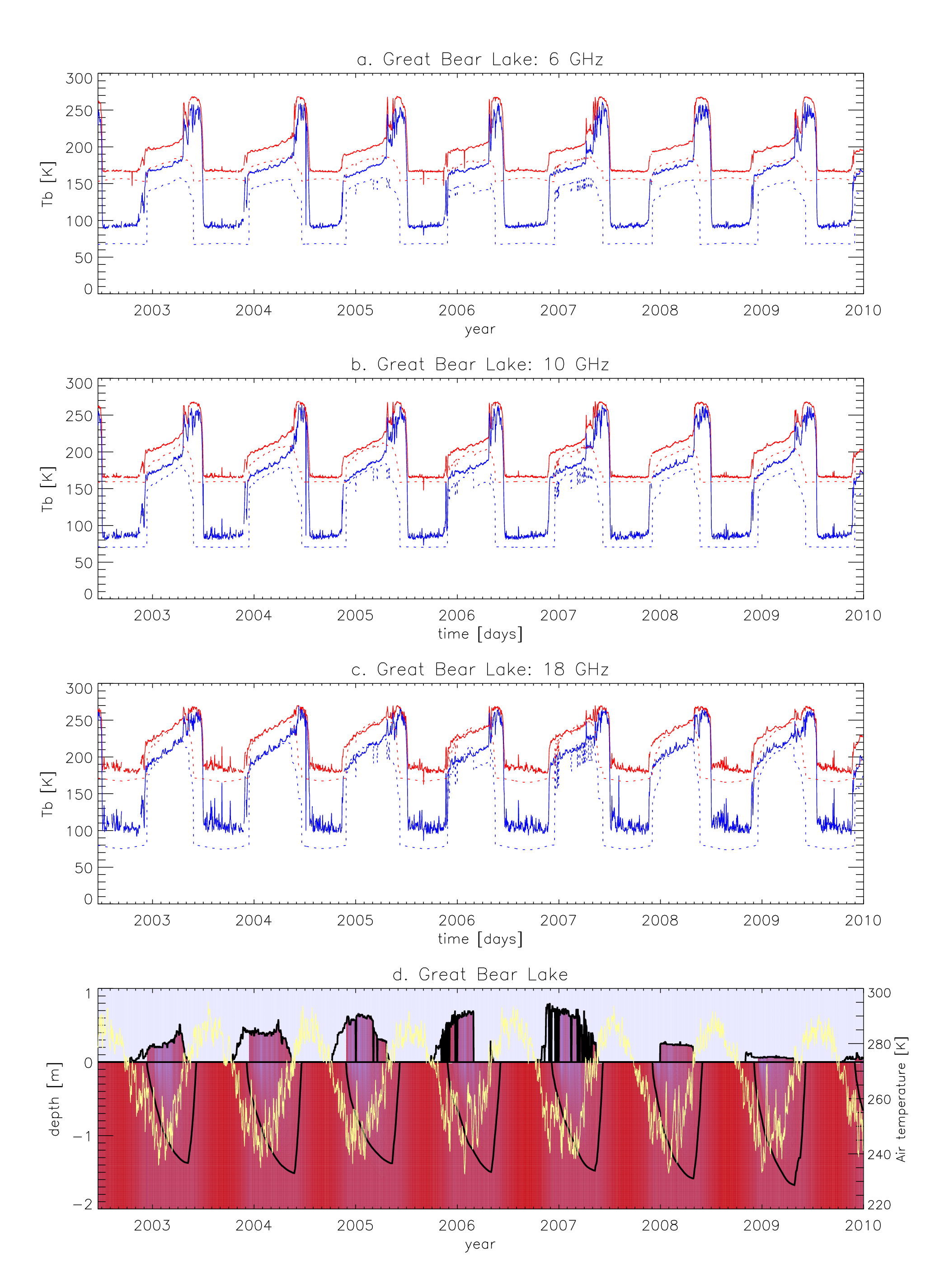
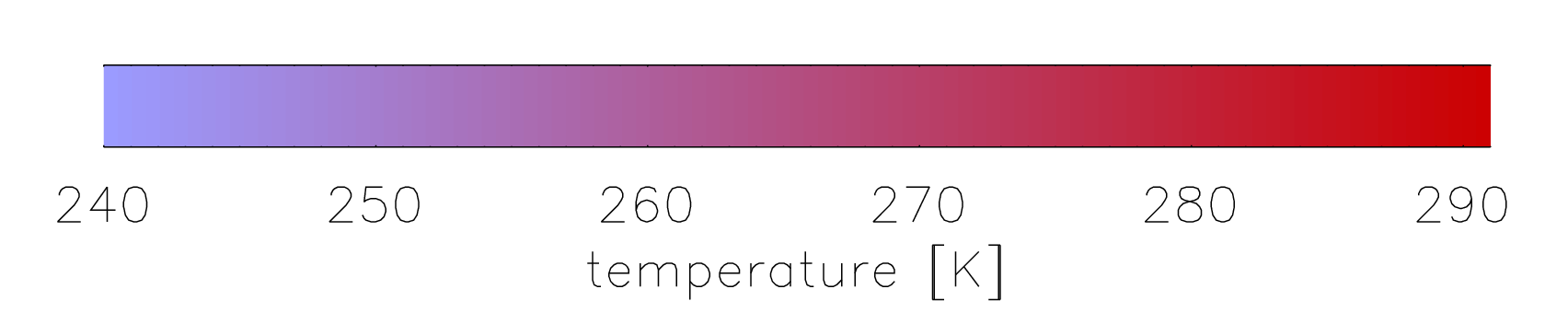
Figure 1: (a), (b) and (c): Time series of measured versus modelled brightness temperatures over the Great Bear Lake, 6, 10 and 18 GHz, respectively. (d): Ice thickness (black lines), snow depth (black lines), ice and water temperature (shading) and air temperature (yellow line).

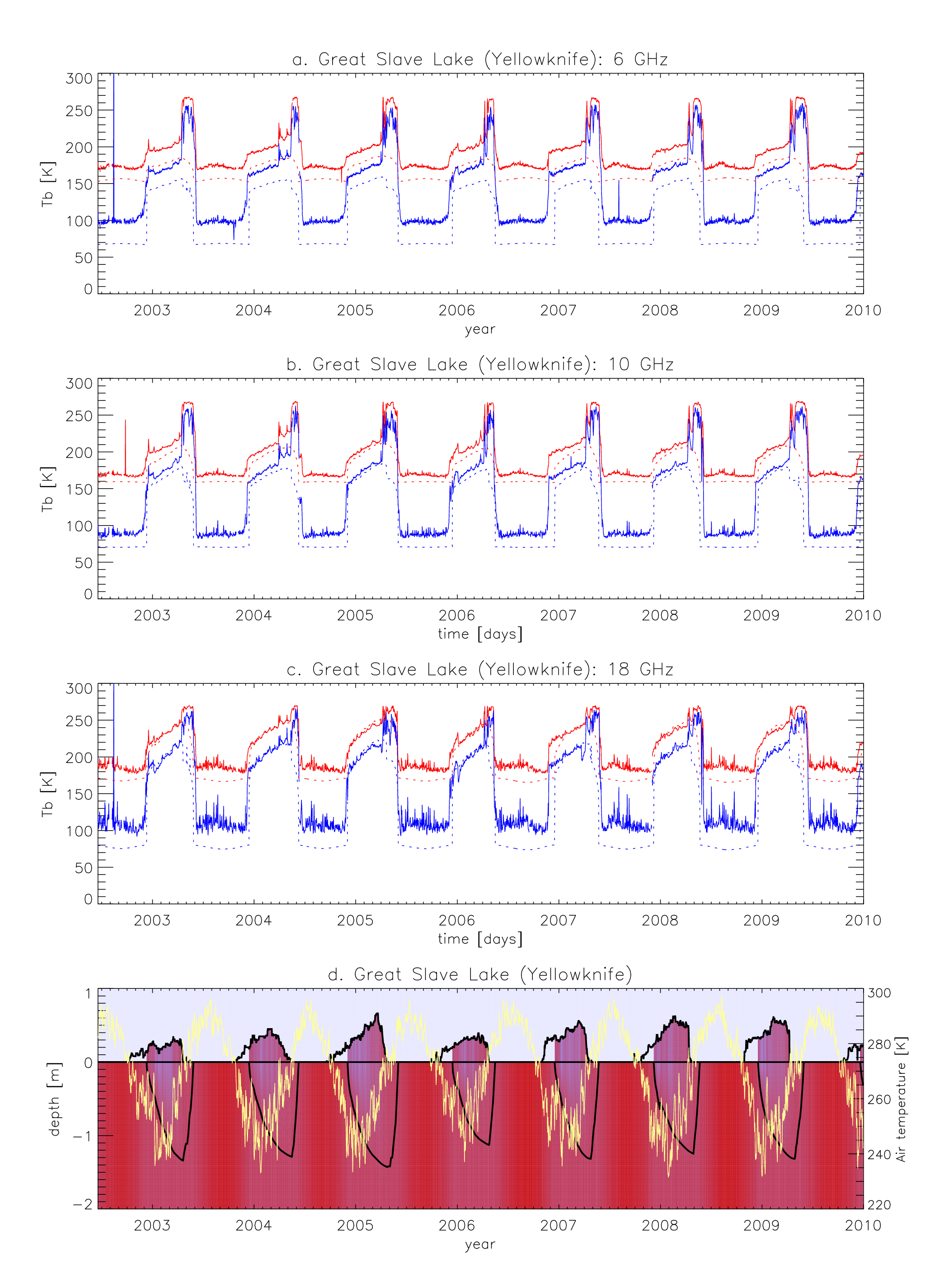
Figure 2: (a), (b) and (c): Time series of measured versus modelled brightness temperatures over the Great Slave Lake near Yellowknife, 6, 10 and 18 GHz, respectively. (d): Ice thickness (black lines), snow depth (black lines), ice and water temperature (shading) and air temperature (yellow line).

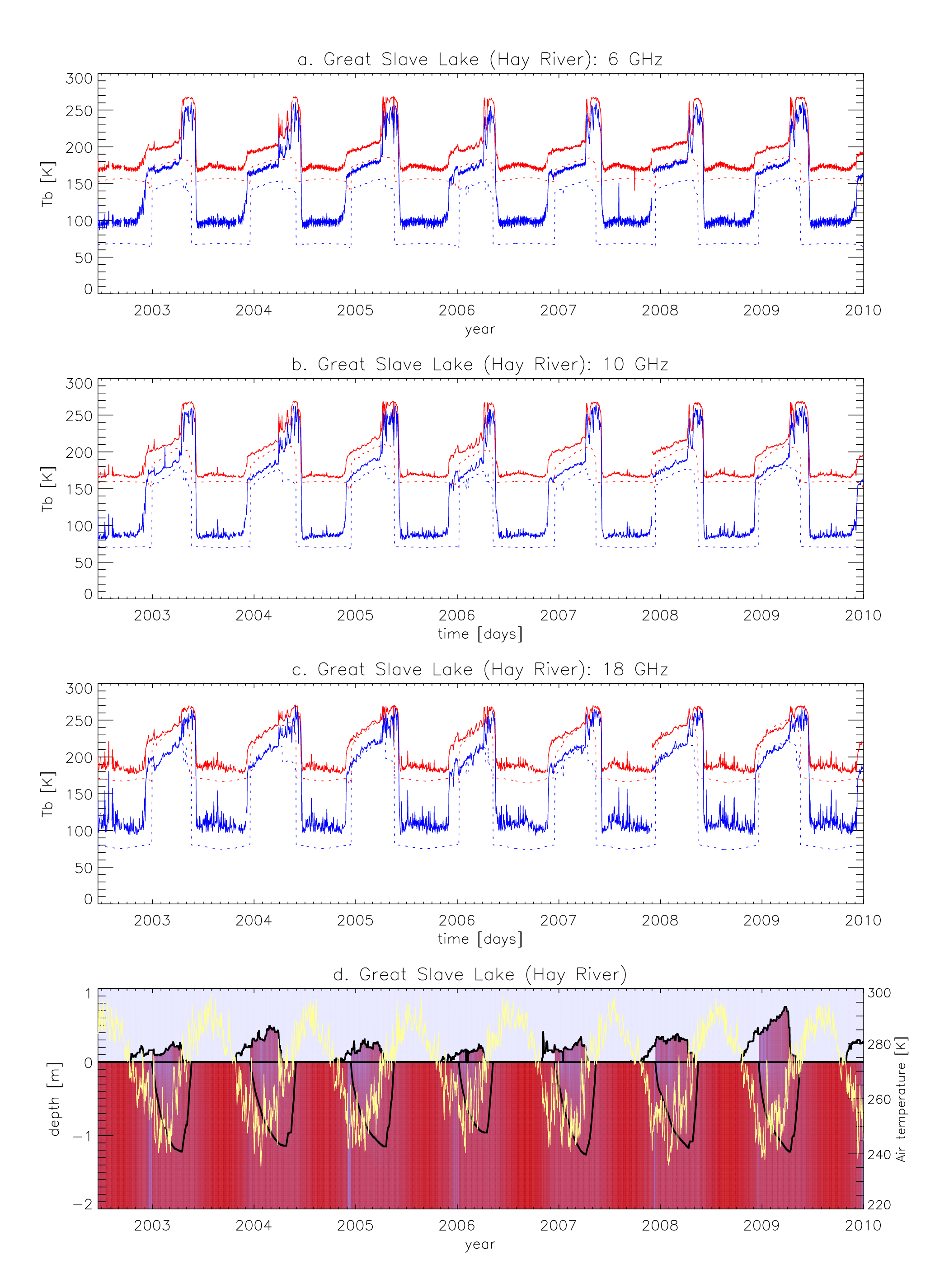
Figure 3: (a), (b) and (c): Time series of measured versus modelled brightness temperatures over the Great Slave Lake near Hay River, 6, 10 and 18 GHz, respectively. (d): Ice thickness (black lines), snow depth (black lines), ice and water temperature (shading) and air temperature (yellow line).

The main results are summarized in Figures 1, 2 and 3. The model shows considerable skill at predicting Tbs over the Great Bear and Great Slave Lakes, except during the melt season. Using only temperature, the model has limited predictive power over open water at 6 GHz. At 10 GHz, the model shows very little variation over open water, while at 18 GHz, modelled Tbs are negatively correlated with measured, showing a lowering of Tb during warm weather where the measured values are raised.

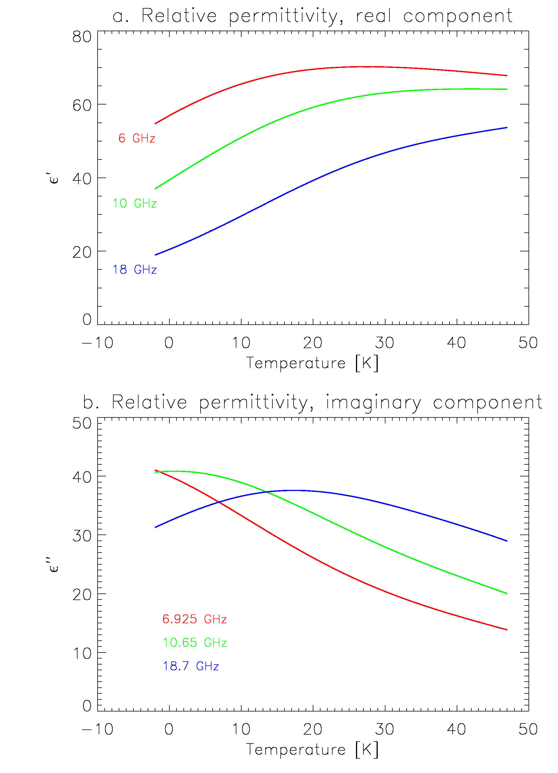
Figure 4: Modelled complex relative permittivity of pure water at different temperatures.

The modelled decrease in Tb with increasing temperature over open water at 18 GHz can be explained by the modelled relative permittivities, shown in Figure 4. These have been simulated using a Debye relaxation curve (Ulaby et al., 1986) and rise much more steeply at 18 GHz than at the other channels, although why the resulting Tbs disagree with the actual values is unclear.

Figure 5: Scatterplots of ice during the winter season ((a) and (b), h and v polarizations resp.) and open water during the summer months ((c) and (d), h and v polarizations resp.) for 6 GHz.

Figure 6: Scatterplots of ice during the winter season ((a) and (b), h and v polarizations resp.) and open water during the summer months ((c) and (d), h and v polarizations resp.) for 10 GHz.

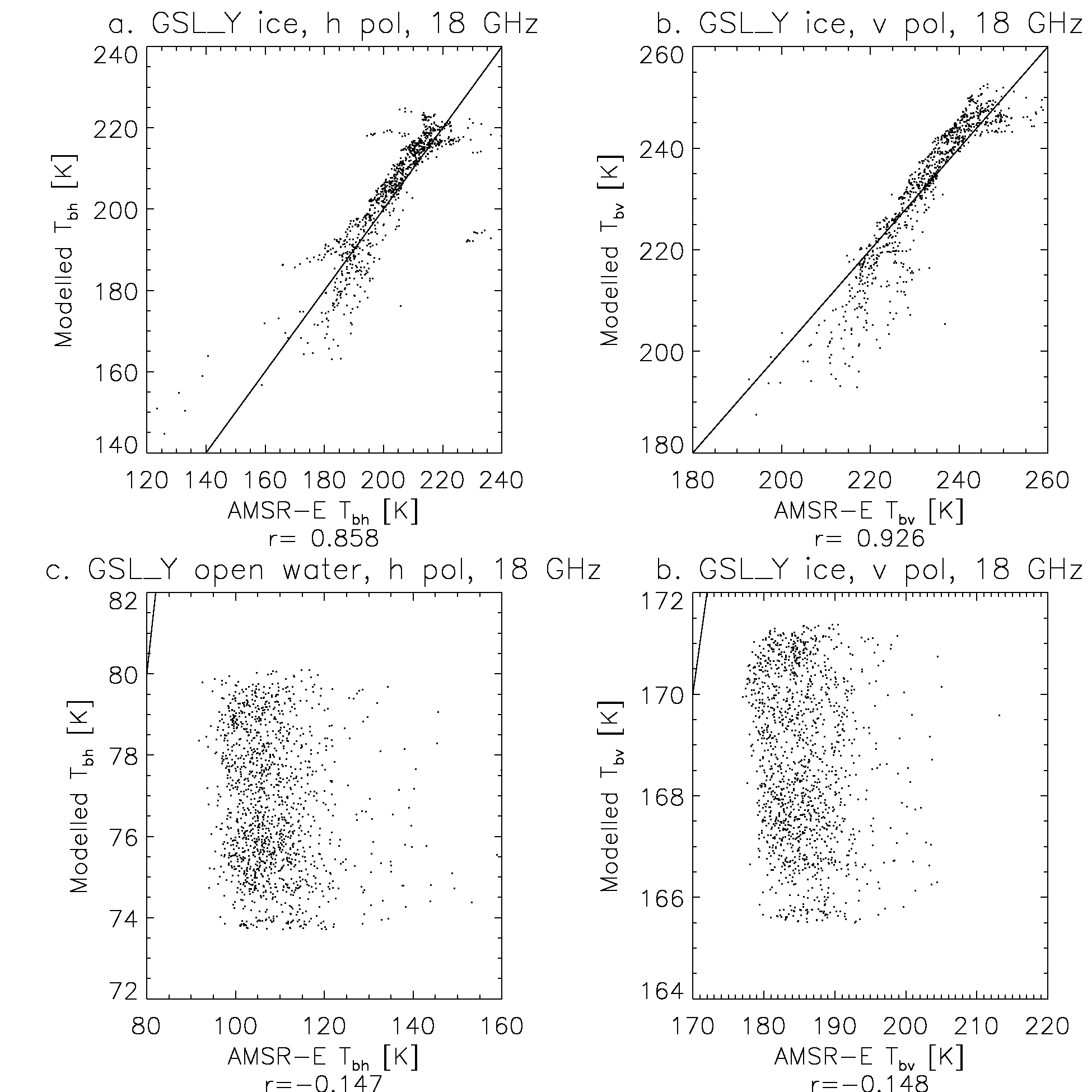
Figure 7: Scatterplots of ice during the winter season ((a) and (b), h and v polarizations resp.) and open water during the summer months ((c) and (d), h and v polarizations resp.) for 18 GHz.

The skill of model predictions over the Great Slave Lake near Yellowknife for both ice-covered and open water is outlined by the scatterplots in Figures 5, 6 and 7 for 6, 10 and 18 GHz respectively. There are two seasons during which the model suffers and both of these have been excluded from the comparison as they are in some sense beyond the scope of the model. Measured Tbs show a marked increase during the melt season, something which is not reflected in the models. This is thought to be caused by dirt within the snow which is exposed as it melts, producing a Tb signature closer to that of soil than of ice or snow. In Kang et al. (2010), melt onset is identified by a succession of four or more days during which the air temperature rises above freezing. Here we use a more basic technique to select the values of interest, by simply choosing points where the measured Tbs are between 140 and 200 K at 6 GHz, horizontal polarization.

A similar technique is used to select open water points in which Tbs are restricted to between 70 and 110 K at 10 GHz, horizontal polarization. This effectively removes the beginning of fall freeze-up, during which the lake may be only partially ice-covered or contain substantial amounts of crystallized ice particles (frazil), neither circumstance of which is encompassed by the ice growth model. For a simple method of modelling mixed surface types, see (Mills and Heygster, 2011b).

Were the model results to be linearly re-calibrated (see below), the residuals for the vertical polarization over open water, 6 GHz, and over ice, 18 GHz, would be 2.4 K and 0.78 K, respectively.

Table 1: Brightness temperature biases in Kelvin from the previous study over Lake Superior for both uncorrected model results and those that have been corrected for atmospheric effects. For the ice case, the modelled values are for 1 m ice thickness.

Channel	Lake Ice		Open water
	uncor.	cor.	uncor.	cor.
6.925 h	-11.8	-9.3	-16.7	-10.0
6.925 v	-6.6	-5.0	-7.0	-3.7
10.65 h	-4.5	-1.6	-18.9	-9.5
10.65 v	4.8	6.5	-6.3	-1.6
18.7 h	8.6	15.8	-28.0	4.3
18.7 v	22.8	25.3	-9.3	6.8

Table 2: Brightness temperature biases in Kelvin for the current study over the Great Slave Lake near Yellowknife.

Channel	Lake ice	Open water
6.925 h	-22.4	-31.7
6.925 v	-20.7	-17.0
10.65 h	-9.7	-18.3
10.65 v	-10.6	-9.5
18.7 h	1.0	-31.5
18.7 v	-0.5	-16.9

While the emissivity model appears to have considerable predictive power, it is not well calibrated. Only at 18 GHz do the ice brightness temperatures show relatively little bias. This is a consistent problem across many of the studies modelling microwave emissivity conducted by this author (Heygster et al., 2009; Mills and Heygster, 2011c; Mills, 2012). Other studies have also shown biases and other discrepancies with modelled snow and ice brightness temperatures, depending on the type of model used (Winebrenner et al., 1992; Tedesco et al., 2006). Possible explanations include calibration problems in the radiometer, as in Mills and Heygster (2011c), the influence of weather and factors not included in the model such as scattering, ice ridging, impurities in the ice and snow cover. In Mills (2012), weather was crudely accounted for using a parameterized correction scheme (Wentz and Meissner, 2000). This step improved the prediction of open water emissivity as seen in Table 1 but did little to improve the prediction over ice as the relative biases between different frequencies remained similar and in fact became slightly worse. Biases over ice were calculated for a modelled ice thickness of 1 m and uniform, freezing temperature within the ice sheet.

Consider, for comparison, the equivalent biases for the current study, shown in Table 2. In both this and the previous study, the spread between the 6 and 8 GHz horizontally-polarized channels is between 23 and 25 K.

3 Conclusion

Lake ice brightness temperatures over the Great Bear and Great Slave Lakes were simulated at 6.925, 10.65 and 18.7 GHz using radiative transfer from ice thicknesses and temperatures from the Canadian Lake Ice Model (ClIMo). These were compared with measurements from the Advanced Microwave Scanning Radiometer (AMSR) on the Earth Observational Satellite (EOS). Modelled ice Tbs were found to have strong predictive power when compared with measurements except during the melt season. Modelled open water Tbs had some predictive power, but not during fall freeze-up and not at 10 GHz, while those at 18 GHz were negatively correlated with measured values. All Tbs except at 18 GHz over ice, were found to have significant bias. The source of this bias is as yet unclear and further work needs to be done. The interaction of electro-magnetic radiation with matter is a fundamental problem in physics and to date, most of the emissivity models for ice and snowpack are rather ad-hoc, the current one being no exception. The study of Mills and Heygster (2011c) that investigated the effect of ice ridging on the microwave signature suggest that a more rigorous model based on wave interaction rather than simple line-of-sight would have better predictive power. It is hoped that future studies can delve more deeply into the theory and develop more reliable models for ice electromagnetic properties as well as combine these with more sophisticated ice growth models.

References

- Cox and Weeks (1988) Cox, G. and Weeks, W. (1988). Numerical simulations of the profile properties of undeformed first-year sea ice during the gowth season. Journal of Geophysical Research, 93(C10):12499–12460.
- Duguay et al. (2003) Duguay, C. R., Flato, G. M., Jeffries, M. O., Menard, P., Morris, K., and Rouse, W. R. (2003). Ice-cover variability on shallow lakes at high latitudes: model simulations and observations. Hydrological Processes, 17:3465–3483.
- Heygster et al. (2009) Heygster, G., Hendricks, S., Kaleschke, L., Maass, N., Mills, P., Stammer, D., Tonboe, R. T., and Haas, C. (2009). L-Band Radiometry for Sea-Ice Applications. Technical Report final report for ESA/ESTEC Contract N. 21130/08/NL/EL, Institute of Environmental Physics, University of Bremen.
- Kang et al. (2010) Kang, K.-K., Duguay, C. R., Howell, S. E. L., Derksen, C. P., and Kelly, R. E. J. (2010). Sensitivity of AMSR-E Brightness Temperature to the Seasonal Evolution of Lake Ice Thickness. IEEE Geoscience and Remote Sensing Letters, 7(4):751–755.
- Mills (2012) Mills, P. (2012). Microwave emissivity of freshwater ice–lake ice and antarctic icepack–radiative transfer simulations versus satellite radiances. Technical Report arxiv:1202.4095v1, Peteysoft Foundation.
- Mills and Heygster (2011a) Mills, P. and Heygster, G. (2011a). Retrieving sea ice concentration from smos. IEEE Geoscience and Remote Sensing Letters, 8(2):283–287.
- Mills and Heygster (2011b) Mills, P. and Heygster, G. (2011b). Sea ice brightness temperature as a function of ice thickness: Computed curves for AMSR-E and SMOS (frequencies from 1.4 to 89 GHz). Technical Report DFG project HE-1746-15, University of Bremen.
- Mills and Heygster (2011c) Mills, P. and Heygster, G. (2011c). Sea ice emissivity modelling at L-band and application to Pol-Ice campaign field data. IEEE Transactions on Geoscience and Remote Sensing, 49(2):612–627.
- Sihvola and au Kong (1988) Sihvola, A. H. and au Kong, J. (1988). Effective Permittivity of Dielectric Mixtures. IEEE Transactions on Geoscience and Remote Sensing, 26(4).
- Tedesco et al. (2006) Tedesco, M., Kim, E. J., England, A. W., Roo, R. D., and Hardy, J. P. (2006). Intercomparison of Electromagnetic Models for Passive Microwave Remote Sensing of Snow. IEEE Transactions on Geoscience and Remote Sensing, 44(10).
- Ulaby et al. (1986) Ulaby, F. T., Moore, R. K., and Fung, A. K., editors (1986). Microwave Remote Sensing: Active and Passive, Volume III, From Theory to Applications. Artech House, Norwood, MA.
- Wentz and Meissner (2000) Wentz, F. J. and Meissner, T. (2000). AMSR Ocean Algorithm. Algorithm Theoretical Basis Document RSS Tech. Proposal 121599A-1, Remote Sensing Systems, Santa Rosa CA. prepared for NASA Goddard.
- Winebrenner et al. (1992) Winebrenner, D. P., Bredow, J., Fung, A. K., Drinkwater, M. R., Nghiem, S., Gow, A. J., Perovich, D. K., , Grenfell, T. C., Han, H. C., Kong, J. A., Lee, J. K., Mudaliar, S., Onstott, R. G., Tsang, L., and West, R. D. (1992). Microwave sea ice signature modelling. In Microwave Remote Sensing of Sea Ice, number 68 in Geophysical Monographs, chapter 8, pages 137–175. American Geophysical Union.