The effects of viewing angle on the mass distribution of exoplanets

Abstract

We present a mathematical method to statistically decouple the effects of unknown inclination angles on the mass distribution of exoplanets that have been discovered using radial-velocity techniques. The method is based on the distribution of the product of two random variables. Thus, if one assumes a true mass distribution, the method makes it possible to recover the observed distribution. We compare our prediction with available radial-velocity data. Assuming the true mass function is described by a power-law, the minimum mass function that we recover proves a good fit to the observed distribution at both mass ends. In particular, it provides an alternative explanation for the observed low-mass decline, usually explained as sample incompleteness. In addition, the peak observed near the the low-mass end arises naturally in the predicted distribution as a consequence of imposing a low-mass cutoff in the true-distribution. If the low-mass bins below 0.02M_J are complete, then the mass distribution in this regime is heavily affected by the small fraction of lowly inclined interlopers that are actually more massive companions. Finally, we also present evidence that the exoplanet mass distribution changes form towards low-mass, implying that a single power law may not adequately describe the sample population.

1. Introduction

Samples of exoplanetary systems are increasing rapidly thanks to new ground and space-based dedicated surveys, thus enabling investigation of their statistical properties. One of these properties is the planetary mass distribution, a key aspect needed to understand the origin of exoplanets and its relation to the initial mass function. Currently, radial-velocity (RV) detections (e.g. Mayor et al., 1983; Butler et al., 1996; Jones et al., 2010) have provided the largest sample of unconstrained systems. However, the RV technique does not provide masses directly because the line-of-sight inclination angles, $i$, cannot be measured unless complementary observations are carried out, for instance transit photometry (Henry et al., 2000) or astrometry (Benedict et al., 2006). Thus, all masses measured with this technique are indeed ’minimum’ planet masses, $M_{\rm obs}=M_{\rm T}\sin{i}$, where $M_{\rm T}$, the ’true’ planet mass, is not known a priori.

Understanding the true mass distribution rather than the minimum mass distribution will allow modelers to compare their mass distributions against a function that is free from one of the largest sources of uncertainty (see Mordasini et al., 2009; Ida & Lin, 2005). Also, the $\sin i$ degeneracy that plagues RV signals means we can never be fully sure that any individual signature is planetary in nature from the Doppler data alone. This has consequences for a number of aspects of planetary, brown dwarf, and low-mass star studies that deal with inferences drawn from a RV dominated mass distribution. A prime example of this would be the proper location in mass of the planet-brown dwarf boundary (see Sahlmann et al., 2011), which allows one to clarify the status of an object as either a planet or a brown dwarf (e.g. Jenkins et al. 2009a, ), and will help us to better understand the formation mechanisms of both classes of objects.

It is thought that the $\sin{i}$ correction is of order unity and would preserve the power-law shape of the observed mass distribution (e.g., Jorissen et al., 2001; Tabachnik & Tremaine, 2002; Hubbard et al., 2007; Morton & Johnson 2011). However, no proof has been provided to substantiate this. Methods to recover the $M_{\rm T}$ distribution from the observed minimum-mass data have been proposed based on: (1) numerically solving an Abel-type integral equation that relates observed and true mass distributions (Jorissen et al., 2001); (2) analytically finding the distribution that maximizes the likelihood of having a given set of minimum masses (Zucker & Mazeh, 2001); (3) comparing cumulative distributions of projected and de-projected data with non-parametric statistical tools (Brown, 2011); and (4) using the physics of multi-planet systems to resolve the $\sin{i}$ correction (Batygin & Laughlin, 2011). With the exception of (4), which is a theoretical prediction, these methods are non-parametric, i.e., they do not assume an a priori model of the data. However, they also suffer from some drawbacks like the need to smooth the data (1 and 3), or the complexity of introducing observational limits (2).

In this paper we present an alternative method to statistically decouple the $\sin i$ dependence in observed exoplanet mass functions. The method is based on the expected distribution of the product of two continuous and independent random variables. Its parametric nature requires an assumption on the shape of the underlying ($M_{\rm T}$) distribution; but, on the other hand, it offers the possibility of introducing observational constraints in a straightforward fashion. The mathematical problem, applied to planet mass distributions, is stated in § 2, and its solution presented in § 3. In § 4 the method is implemented on two example distributions and in § 5 we make a comparison with observational data. In § 6 we look at the significance of the shape of the true mass distribution and how this may affect current models of planet formation and evolution. Finally, in § 7 we summarize the results.

2. The problem and our concept

The problem can be summarized as follows: given an analytical model of the distribution of true planetary masses, is it possible to obtain the distribution of minimum-masses analytically by assuming a random distribution of inclination angles? The answer to this question is yes, and relies on computing the probability density function (PDF) of the product of two random variables. The problem of finding the PDF of the product of two random variables was first solved by Rohatgi (1976) but its implementation relied on knowledge of the joint PDF of the two variables. In this paper we apply the approach followed by Glen et al. (2004), which uses the individual PDFs of the two random variables.

To do so, let $X$, $Y$, and $Z$ be random variables, such that

$$X=M_{\rm T}$$ (1)

$$Y=\sin{i}$$ (2)

$$Z=XY~{}.$$ (3)

The above equations state that $X$ takes the value of any exoplanetary mass, $M_{\rm T}$, $Y$ takes the value of any correction by inclination (viewing) angle $i$, $\sin{i}$, and $Z$ takes the value of any possible product $M_{\rm T}\sin{i}$. Let also $f_{X}$, $f_{Y}$, and $f_{Z}$ be their respective probability density functions (PDF). We wish to obtain $f_{Z}$, a prediction for the observed distribution of ’minimum’ masses, given $f_{X}$ (an assumption for the true mass distribution) and $f_{Y}$ (which can be calculated analytically).

3. Solution

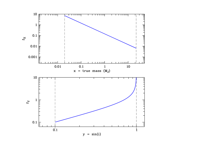
Figure 1.— Top panel: PDF of $X$ describing true masses, with $\alpha=0$$,m_{\rm min}=0.02$ and $m_{\rm max}=22$ M_J. Bottom panel: PDF of $Y$ describing $\sin i$ corrections, with $i$ values drawn from a uniform distribution in the range [5.7,90.0] degrees.

3.1. PDF of $X$

Let $f_{X}$ represent the distribution of planet true masses. For simplicity, we assume $f_{X}$ is well described by a power-law. We define a power-law of index $-(1+\alpha)$, such that it is normalized over the mass interval $[m_{\rm min},m_{\rm max}]$, defined to be the minimum and maximum true masses. Note that a minimum non-zero mass avoids a diverging integral, which is a condition for $f_{X}$ to be normalized. Thus, $f_{X}$ becomes

$$f_{X}(x)~{}dx=\begin{cases}A_{X}x^{-\alpha-1}~{}dx,&0<m_{\rm min}<x<m_{\rm max}\\ 0,&\text{otherwise,}\end{cases}$$ (4)

where $x$ represents true masses, $A_{X}\equiv\alpha/(m_{\rm min}^{-\alpha}-m_{\rm max}^{-\alpha})$ is a normalization constant and $\alpha>-1$. If $\alpha=0$, then $A_{X}=(\ln{(m_{\rm max}/m_{\rm min})})^{-1}$. It is important to note that $X$ can be treated as a continuous variable and that the present analysis does not require that masses be normalized (i.e., $x$ can be in any units). An example of this PDF, representing the true mass distribution, is shown in the top panel of Fig. 1.

3.2. PDF of $Y$

Consider randomly distributed inclination angles, $i$. The observed inclination angles can be shown to be distributed like $\sin{i}$, over the interval $[0,\frac{\pi}{2}]$. This is straightforward to see in spherical coordinates (e.g., Ho & Turner 2011) and implies that higher inclination angles (edge-on) are more probable than lower ones (pole-on).

To get $f_{Y}$ for a $\sin{i}$-distribution of angles, let $y=\sin{i}$. Then $i=\arcsin{y}$, with $i\in[0,\frac{\pi}{2}]$. The corresponding cumulative distribution (CDF) is given by $1-\cos{i}$. Thus, the differential of this CDF, $d(1-\cos{[i]})=d(1-\cos{[\arcsin{y}]})$ gives $f_{Y}$:

$$f_{Y}(y)~{}dy=\frac{y}{\sqrt{1-y^{2}}}~{}dy,\hskip 28.45274pt0<y<1.$$ (5)

The above equation considers all possible angles. However, it may be useful to define a minimum inclination angle, $i_{\rm min}$, to account for possible selection effects when comparing with real data. In this case $f_{Y}$ becomes

$$f_{Y}(y)~{}dy=A_{Y}\frac{y}{\sqrt{1-y^{2}}}~{}dy,\hskip 28.45274pt\sin{i_{\rm min}}<y<1.$$ (6)

where $A_{Y}\equiv 1/\sqrt{1-\sin{(i_{\rm min})}^{2}}$ is a normalization constant. An example of this PDF, representing the $\sin i$ distribution, is shown in the bottom panel of Fig. 1

3.3. PDF of $Z$

Having defined $f_{X}$ and $f_{Y}$, the PDF of random variables $X$ and $Y$, we can now calculate $f_{Z}$, the PDF of the product $XY$. Following Glen et al. (2004)’s solution for the PDF of the product of two continuous and independent random variables, and also considering the above boundaries, $f_{Z}(z)$ can be expressed as

$$f_{Z}(z)=\begin{cases}\int\limits_{m_{\rm min}}^{z/\sin{i_{\rm min}}}f_{Y}(\frac{z}{u})f_{X}(u)\frac{1}{u}du,&m_{\rm min}\sin{i_{\rm min}}<z<m_{\rm min},\\ \int\limits_{z}^{z/\sin{i_{\rm min}}}f_{Y}(\frac{z}{u})f_{X}(u)\frac{1}{u}du,&m_{\rm min}<z<m_{\rm max}\sin{i_{\rm min}},\\ \int\limits_{z}^{m_{\rm max}}{f_{Y}(\frac{z}{u})f_{X}(u)\frac{1}{u}du},&m_{\rm max}\sin{i_{\rm min}}<z<m_{\rm max},\end{cases}$$ (7)

provided that $m_{\rm min}<m_{\rm max}\sin{i_{\rm min}}$. This condition is the equivalent of setting a lower limit on $i$, such that pole-on orbits, producing very large corrections, are excluded from the observed sample. It also determines three ’validity regions’.

Replacing Eq. 7 with Equations 4 and 6, after some algebra and getting rid of the integration limits for a moment, Eq. 7 reads:

$$f_{Z}(z)=A_{X}A_{Y}z\int\frac{u^{-\alpha-2}}{\sqrt{u^{2}-z^{2}}}du~{}.$$ (8)

For any value of $\alpha$, the improper integral in Eq. 8 has a primitive in terms of ${}_{2}F_{1}$, the first hypergeometric function (Abramowitz & Stegun 1964). From Eq. 7, note also that one important property of $f_{Z}$ is that it vanishes at the boundaries $z=m_{\rm min}\sin{i_{\rm min}}$ and $z=m_{\rm max}$, meaning that the observed mass distribution must have a peak. This has important consequences when interpreting distributions of real data (see § 6).

In conclusion, the problem stated in § 2 is formally solved for the distributions described in § 3.1 and § 3.2. Indeed, Eq. 7 is valid for any true mass distribution (i.e., not only for a power-law) but in general the evaluation of $f_{Z}$ will require numerical integration.

4. Examples

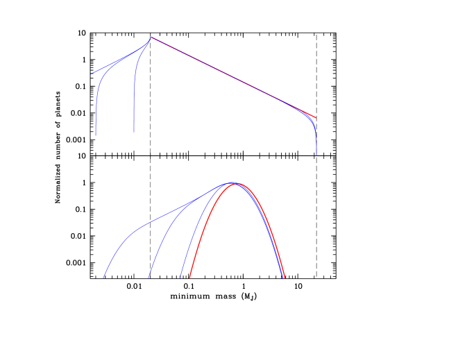
Figure 2.— Top panel: power-law distribution of true masses ($f_{X}$; red curve) with $m_{\rm min}=0.02$ M_J and $m_{\rm max}=22$ M_J, and corresponding predictions of minimum-mass distributions ($f_{Z}$; blue curves) for various minimum inclination angles, $i_{\rm min}=0.57$, $5.7$, and $30.0$ degrees. Bottom panel: same as above but for a log-normal distribution of true masses, $f_{X}(x)=\frac{1}{x\sigma\sqrt{2\pi}}\exp{-\frac{(\ln{x}-\mu)^{2}}{2\sigma^{2}}}$ with $\mu=0$ and $\sigma=0.5$.

We now evaluate numerically two examples of true mass distributions: a power-law and a log-normal distribution.

For the power-law introduced in §3.1 and used to derive Eq. 8, the case $\alpha=0$ is easy to evaluate (and will allow us to perform a quick comparison with RV data in the next Section). Replacing with $\alpha=0$ and integrating Eq. 8, the predicted minimum-mass distribution becomes:

$$f_{Z}(z)dz=\frac{A_{X}A_{Y}}{z}\times\begin{cases}\left[\frac{\sqrt{(z/\sin{i_{\rm min}})^{2}-z^{2}}}{z/\sin{i_{\rm min}}}-\frac{\sqrt{m_{\rm min}^{2}-z^{2}}}{m_{\rm min}}\right]dz,&m_{\rm min}\sin{i_{\rm min}}<z<m_{\rm min},\\ \left[\frac{\sqrt{(z/\sin{i_{\rm min}})^{2}-z^{2}}}{z/\sin{i_{\rm min}}}\right]dz,&m_{\rm min}<z<m_{\rm max}\sin{i_{\rm min}},\\ \left[\frac{\sqrt{m_{\rm max}^{2}-z^{2}}}{m_{\rm max}}\right]dz,&m_{\rm max}\sin{i_{\rm min}}<z<m_{\rm max}.\\ \end{cases}$$ (9)

The function $f_{Z}$ represents the predicted distribution of minimum-masses if the true mass distribution is proportional to $M_{\rm T}^{-1}$.

The top panel of Fig. 2 shows $f_{Z}$ for various minimum inclination angles (blue curves; $i_{\rm min}=0.57$, $5.7$, and $30.0$ degrees). For reference, the underlying distribution of true masses, $f_{X}$, is also shown (red curve), where we have set $m_{\rm min}=0.02$ M_J and $m_{\rm max}=22$ M_J. The effect of the $\sin{i}$ correction is evident at both mass ends of the predicted distribution, as objects in any mass bin ’migrate’ to lower-mass bins in the minimum mass distribution.

However, the shape of the low-mass tail ($z<m_{\rm min}$) is affected mostly by the inclusion of large $\sin i$ corrections, i.e., lowly-inclined systems. This is readily seen from the fact that $f_{Z}$ converges to $f_{X}$ in the limit $\sin{i_{\rm min}}\approx 1$. Thus, in general, the observed distribution of a true mass power-law distribution (with boundaries) should show a decrease at the low-mass end.

The same effects are observed if a log-normal distribution is used instead of a power-law. The bottom panel of Fig. 2 shows such a distribution (same color codes for the true and predicted mass distributions and same $i_{\rm min}$ values), where Eq. 7 has been integrated numerically using

$$f_{X}(x)=\frac{1}{x\sigma\sqrt{2\pi}}\exp{-\frac{(\ln{x}-\mu)^{2}}{2\sigma^{2}}}$$ (10)

with $\mu=0$ and $\sigma=0.5$.

We conclude by emphasizing that setting a particular value of $i_{\rm min}$ simulates observational selection effects, meaning that the model mimics observational samples which have missed objects at angles below that limit. Fig. 2 shows that including those lowly-inclined systems, despite them being less probable, induces dramatic changes in the shape of the predicted distribution at the low-mass end.

We now proceed to compare our models with RV data.

5. Comparison with observational data

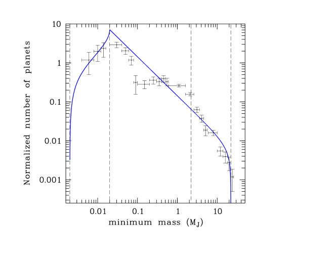
Figure 3.— Observed distribution of minimum masses for a sample of 643 RV discovered exoplanets (data taken from http://exoplanet.eu as of October 17 2011). Bin sizes were arbitrarily chosen to have a roughly equal number of systems. Overlaid is the model of minimum masses given by Eq. 9 and obtained from an assumed true mass distribution with the following parameters: $f(M_{\rm T})\propto M_{\rm T}^{-1}$, $m_{\rm min}=0.02$ M_J, $m_{\rm max}=22$ M_J. The predicted minimum-mass distribution was set to have $\sin{i_{\rm min}}=0.1$. The dashed lines mark the validity regions in Eq. 9

Fig. 3 displays the observed distribution of minimum masses (Schneider et al. 2011; RV data on 643 planets as of October 17 taken from http://exoplanet.eu). Bin sizes were arbitrarily chosen to have a roughly equal number of systems. Overlaid is the model prediction of minimum masses given by Eq. 9, i.e., the prediction that results from assuming a true mass distribution of the form $\propto M_{\rm T}^{-1}$. We have chosen the following physical parameters for the true mass distribution: $m_{\rm min}=0.02$ M_J and $m_{\rm max}=22$ M_J, where the lower limit is chosen from observation and the upper limit marks the planetary-brown dwarf mass boundary (Sahlmann et al. 2011). To simulate observational selection effects, $\sin{i_{\rm min}}=0.1$ was chosen. We emphasize that these parameters are not the result of a fit, but were adjusted manually to attempt a best match to the data.

It can be seen that the power-law part of the predicted curve (Fig. 3) only poorly fits the data. However, interestingly enough, both of its extremes do seem to better reproduce the data.

At the low-mass limit ($z<0.02$ M_J) the model describes mass-bins which are not ’occupied’ in the true mass distribution. As already mentioned, the shape of this tail is affected mostly by the inclusion of large $\sin i$ corrections, i.e., lowly-inclined systems, which in turn produce a decrease at the low-mass end of the observed distribution. Such a decrease mimics observational effects on the data like those ones induced by incompleteness (Udry & Santos, 2007), as we discuss further in next Section.

At the high-mass end, there is no apparent reason for a systematic lack of observed systems. Here the data shows a decline which is also in good agreement with our model’s prediction. However, the small number of systems precludes any firm conclusion.

An interesting feature that appears in the data between the high and low-mass ends of the distribution is a deficit that is not well described by the power law model prediction. Around 0.1 M_J the data drop and then quickly turnover to rise again, creating a mass distribution paucity in the data. Given we expect this mass regime to be fairly well sampled by current RV surveys, this feature may indicate that more than a single power law is needed to describe the full ensemble of planetary masses.

We conclude by emphasizing that the above approach provides a direct comparison with observational data. Assuming the true mass distribution is at least fairly well described by a power-law, we have shown that our solution for the minimum-mass distribution provides a good fit to the observations at both mass ends.

6. Discussion

We have shown that if the true mass distribution is described by a power-law with boundaries, there must be a peak in the observed mass distribution of exoplanets, and therefore this peak has implications for planet formation and evolution models. A peak in the planetary mass distribution tells us that most of the mass of the proto-planetary disk that goes into forming planets, gets locked up in the formation of the larger gas and ice giants. This agrees with the mass distribution of the planets in the solar system.

The widely accepted planetary formation theory is by core accretion and subsequent planet migration (Pollack, 1984; Lin & Papaloizou, 1986) and this model can broadly explain the currently observed population of exoplanets. The peak in the planetary mass distribution needs to be taken into account when comparing the outcomes from core accretion formation models against the observed mass distribution of exoplanets, unless the true mass distribution changes form towards the lowest masses.

One interesting question that arises is, what does the position of the peak in the mass distribution tell us and what does it mean? As we have seen in Fig. 3, our true mass distribution model can provide a good fit to the observed mass distribution of the current population of exoplanets, particularly the peak and subsequent decline.

The low-mass peak we find that best describes the observed data is located around 0.02M_J, or $\sim$6.5M_⊕. When we look at systems that have high inclinations, like an observed mass distribution drawn from transiting planets only, we find that for a complete sample, the observed distribution follows the true distribution with no low-mass peak. Therefore, if we assume that the bins are complete below 0.02M_J, then this is the regime where we begin to observe the effects of systems with low inclination angles, and hence large mass corrections.

Here we are assuming we have sampled all angles above a certain limit, $i_{\rm min}$, but our model considers the lower likelihood of observing systems with low inclinations; therefore this tells us something important that even a small fraction of systems with low inclinations can produce large changes in the observed mass distribution in the low-mass regime. This result is in line with the implications of the analysis by Ho & Turner (2011). These authors demonstrate, using Bayesian analysis, that the posterior distribution of angles is determined by the particular true mass distribution and so the latter cannot be simply obtained from the observed one. Unlike Ho & Turner, we deal here with the prior distribution of angles and study its effects on the assumed shape of the true mass distribution; however, both approaches lead to the conclusion that the low inclination systems modify the low-mass end of the observed distribution.

Also, since most of the observed distribution above the 0.02M_J boundary broadly follows the true distribution then small to medium values of $\sin i$ do not affect the overall mass distribution in a large manner. We make it clear that most of the low-mass systems in these bins are genuine rocky planets, but that the small numbers of low-inclination/high-mass interlopers cause a dramatic change to the observed mass distribution, again, assuming that the low-mass bins are complete.

Finally, we do caution that the true mass distribution we are discussing here applies to planets with small semimajor axes ($\leq$4 AU’s or so). The distribution of mass at ever increasing distances from the central star may change the shape of the true mass distribution, but further analysis on this issue is likely to require many more detections like the directly imaged planets around HR8799 (Marois et al., 2008) or planets discovered by microlensing techniques (e.g. Muraki et al., 2011).

7. Summary and outlook

We have applied the formal solution for the PDF of the product of two independent random variables to the observational problem of decoupling the $\sin i$ factor from an observed sample of exoplanet masses. Our approach requires that the true mass distribution is modeled by a continuous function that represents the PDF (within given physical or observational limits).

We have shown that if the true mass function is modeled as a power-law, comparison with observed data of 643 RV planets shows a good match with our method’s prediction, specifically at both mass ends. In particular, the prediction agrees well with the decline observed toward the low-mass end, thus providing an alternative explanation to the turnover being the result of observational biases.

If the low-mass bins below 0.02M_J are assumed to be complete, then we show that the presence of a small number of systems with low inclinations, and hence much larger true masses, heavily affects the distribution in this regime. Such effects are not seen above this mass region where the $\sin i$ values are more modest and hence corrections are smaller, meaning the true distribution is being matched more closely.

We also again note a mass paucity around 0.1 M_J in the observed mass distribution, as the single power law model does not describe this region very well at all. In fact, it may be prudent to examine the mass distribution using more than one function, like a double power law for instance. This may indicate that the mass distribution changes form below around 0.1 M_J, a feature we plan to study more in the future.

In summary, we have provided a practical and intuitive method to decouple the $\sin i$ effect that is inherent to RV samples. The method offers the possibility of introducing observational constraints in a straightforward fashion, in order to compare predictions with current observations.

Current RV surveys are plagued with biases and incompleteness that affect conclusions drawn from analyzing any Doppler data set. For instance, the RV detection method is heavily biased towards the detection of more massive companions on short period orbits, since they induce a larger reflex motion on the host star in comparison with less massive and longer period companions. Therefore, the detection of very low-mass planets is only now being fully realized and requires large data sets and novel detection/characterization methods (e.g. Vogt et al., 2010; Pepe et al., 2011; Anglada-Escude et al., 2012; Jenkins et al., 2012). Hence, studying the low-mass end of the mass distribution is one of the corner-stones of exoplanet research at the present time and will continue to be so in the near future.

References

- Abramowitz & Stegun (1964) Abramowitz, M. & Stegun, I. A., 1964. Handbook of Mathematical functions, Applied Mathematics Series, vol. 55.
- Anglada-Escude et al. (2012) Anglada-Escudé, G., Arriagada, P., Vogt, S. S., Rivera, E. J., Butler, R. P., Crane, J. D., Shectman, S. A., Thompson, I. B., Minniti, D., Haghighipour, N., Carter, B. D., Tinney, C. G., Wittenmyer, R. A., Bailey, J. A., O’Toole, S. J., Jones, H. R. A., Jenkins, J. S. 2012, ApJ, 751, 16
- Barnes et al. (2012) Barnes, J.R., Jenkins, J.S., Jones, H.R.A., Rojo, P., Arriagada, P., Jordan, A., Minniti, D., Tuomi, M., Jeffers, S. V., Pinfield, D. 2012, MNRAS, 424, 591
- Batygin & Laughlin (2011) Batygin, K. & Laughlin, G. 2011, ApJ, 730, 95
- Benedict et al. (2006) Benedict, G. Fritz, McArthur, Barbara E., Gatewood, George, Nelan, Edmund, Cochran, William D., Hatzes, Artie, Endl, Michael, Wittenmyer, Robert, Baliunas, Sallie L., Walker, Gordon A. H., Yang, Stephenson, K urster, Martin Els, Sebastian, Paulson, Diane B. 2006, AJ, 132, 2206
- Brown (2011) Brown, R. A. 2011, ApJ, 733, 68
- Butler et al. (1996) Butler, R. P., Marcy, G. W., Williams, E., McCarthy, C., Dosanjh, P., Vogt, S. S. 1996, PASP, 108, 500
- Butler et al. (2006) Butler, R. P., Wright, J. T., Marcy, G. W., Fischer, D. A., Vogt, S. S., Tinney, C. G., Jones, H. R. A., Carter, B. D., Johnson, J. A., McCarthy, C., Penny, A. J. 2006, ApJ, 646,505
- Borucki et al. (2011) Borucki et al. 2011, ApJ, 736, 19
- Glen, Leemis & Drew (2004) Glen, A. G., Leemis, L. M. & Drew, J. H., 2004, ”Computing the distribution of the product of two continuous random variables,” Computational Statistics & Data Anal ysis, Elsevier, vol. 44(3), pages 451-464, January.
- Henry et al. (2000) Henry, Gregory W., Marcy, Geoffrey W., Butler, R. Paul, Vogt, Steven S. 2000, ApJ, 529, 41
- Ho & Turner (2011) Ho, S., & Turner, E. L. 2011, ApJ, 739, 26
- Ida & Lin (2005) Ida, S., Lin, D. N. C. 2005, ApJ, 626, 1045
- Hubbard et al. (2007) Hubbard, W. B., Hattori, M. F., Burrows, A., & Hubeny, I. 2007, ApJ, 658, 59
- (15) Jenkins, J. S., Jones, H. R. A., Goździewski, K., Migaszewski, C., Barnes, J. R., Jones, M. I., Rojo, P., Pinfield, D. J., Day-Jones, A. C., Hoyer, S. 2009a, MNRAS, 398, 911
- (16) Jenkins, J. S., Ramsey, L. W., Jones, H. R. A., Pavlenko, Y., Gallardo, J., Barnes, J. R., Pinfield, D. J. 2009b, ApJ, 704, 975
- Jenkins et al. (2012) Jenkins, J. S., Jones, H. R. A., Tuomi, M., Murgas, F., Hoyer, S., Jones, M. I., Barnes, J. R., Pavlenko, Y. V., Ivanyuk, O., Rojo, P., Jordán, A., Day-Jones, A. C., Ruiz, M. T., Pinfield, D. J. 2012, ApJ, submitted, arxiv:1207.1012
- Jones et al. (2010) Jones, Hugh R. A., Butler, R. Paul, Tinney, C. G., O’Toole, Simon, Wittenmyer, Rob, Henry, Gregory W., Meschiari, Stefano, Vogt, Steve, Rivera, Eugenio, Laughlin, Greg, Carter, Brad D., Bailey, Jeremy, Jenkins, James S. 2010, MNRAS, 403, 1703
- Jorissen et al. (2001) Jorissen, A., Mayor, M. & Udry, S. 2001, A&A, 379, 992
- Kobayashi et al. (2011) Kobayashi, H., Tanaka, H., Krivov, A.V. 2011, ApJ, 738, 35
- Lin & Papaloizou (1986) Lin & Papaloizou 1986, ApJ, 309, 846
- Mahadevan et al. (2010) Mahadevan, Suvrath, Ramsey, Larry, Wright, Jason, Endl, Michael, Redman, Stephen, Bender, Chad, Roy, Arpita, Zonak, Stephanie, Troupe, Nathaniel, Engel, Leland, Sigurdsson, Steinn, Wolszczan, Alex, Zhao, Bo 2010, SPIE, 7735, 227
- Marois et al. (2008) Marois, C., Macintosh, B., Barman, T., Zuckerman, B., Song, I., Patience, J., Lafreniere D., Doyon, R. 2008, Science, 322, 1348
- Mayor et al. (1983) Mayor, M., Imbert, M., Andersen, J., Ardeberg, A., Baranne, A., Benz, W., Ischi, E., Lindgren, H., Martin, N., Maurice, E., Nordstrom, B., Prevot, L. 1983, A&AS, 54, 495
- Mizuno (1980) Mizuno, H. 1980, PThPh, 64, 544
- Mordasini et al. (2009) Mordasini, C., Alibert, Y., Benz, W., Naef, D. 2009, A&A, 501, 1161
- Morton & Johnson (2011) Morton, T. D., & Johnson, J. A. 2011, ApJ, 738, 170
- Muraki et al. (2011) Muraki, Y., Han, C., Bennett, D. P., et al. 2011, ApJ, 741, 22
- Pepe et al. (2011) Pepe, F., Lovis, C., Ségransan, D., Benz, W., Bouchy, F., Dumusque, X., Mayor, M., Queloz, D., Santos, N. C., Udry, S. 2011, A&A, 534, 58
- Pollack (1984) Pollack 1984, ARA&A, 22, 389
- Ramsey et al. (2008) Ramsey, L. W., Barnes, J., Redman, S. L., Jones, H. R. A., Wolszczan, A., Bongiorno, S., Engel, L., Jenkins, J. 2008, PASP, 120, 887
- Rohatgi (1976) Rohatgi, V. K., 1976, An Introduction to Probability Theory Mathematical Statistics. Wiley, New York.
- Sahlmann et al. (2011) Sahlmann, J., Ségransan, D., Queloz, D., Udry, S., Santos, N. C., Marmier, M., Mayor, M., Naef, D., Pepe, F., Zucker, S. 2011, A&A, 525, 95
- Schneider et al. (2011) Schneider, J., Dedieu, C., Le Sidaner, P., Savalle, R., & Zolotukhin, I., 2011, A&A, 532, 79
- Tabachnik & Tremaine (2002) Tabachnik, S. & Tremaine, S. 2002, MNRAS, 335, 151
- Udry & Santos (2007) Udry, S. & Santos, N. C. 2007, ARA&A, 45, 397
- Vogt et al. (2010) Vogt, Steven S., Wittenmyer, Robert A., Butler, R. Paul, O’Toole, Simon, Henry, Gregory W., Rivera, Eugenio J., Meschiari, Stefano, Laughlin, Gregory, Tinney, C. G., Jones, Hugh R. A., Bailey, Jeremy, Carter, Brad D., Batygin, Konstantin 2010, ApJ, 708, 1366
- Zucker & Mazeh (2001) Zucker, S. & Mazeh, T. 2001, pJ, 562, 1038