1 Introduction

Stochastic optimization algorithms have many desirable features for large-scale machine learning, and accordingly have been the focus of renewed and intensive study in the last several years (e.g., see the papers [26, 4, 10, 30] and references therein). The empirical efficiency of these methods is backed with strong theoretical guarantees, providing sharp bounds on their convergence rates. These convergence rates are known to depend on the structure of the underlying objective function, with faster rates being possible for objective functions that are smooth and/or (strongly) convex, or optima that have desirable features such as sparsity. More precisely, for an objective function that is strongly convex, stochastic gradient descent enjoys a convergence rate ranging from $\mathcal{O}(1/T)$, when features vectors are extremely sparse, to $\mathcal{O}(d/T)$ when feature vectors are dense [11, 19, 12]. Such results are of significant interest, because the strong convexity condition is satisfied for many common machine learning problems, including boosting, least squares regression, support vector machines and generalized linear models, among other examples.

A complementary type of condition is that of sparsity, either exact or approximate, in the optimal solution. Sparse models have proven useful in many application areas (see the overview papers [7, 18, 5] and references therein for further background), and many optimization-based statistical procedures seek to exploit such sparsity via $\ell_{1}$-regularization. A significant feature of optimization algorithms for sparse problems is their mild logarithmic scaling with the problem dimension [20, 27, 10, 30]. More precisely, it is known [20, 27] that when the optimal solution $\theta^{*}$ has at most $s$ non-zero entries, appropriate versions of the stochastic mirror descent algorithm converge at a rate $\mathcal{O}(s\sqrt{(\log d)/T})$. Srebro et al. [28] exploit the smoothness of many common loss functions; in application to sparse linear regression, their analysis yields improved rates of the form $\mathcal{O}(\eta\sqrt{(s\log d)/T})$, where $\eta$ is the noise variance. While the $\sqrt{\log d}$ scaling of the error makes these methods attractive in high dimensions, observe that the scaling with respect to the number of iterations is relatively slow—namely, $\mathcal{O}(1/\sqrt{T})$ as opposed to the $\mathcal{O}(1/T)$ rate possible for strongly convex problems.

Many optimization problems encountered in practice exhibit both features: the objective function is strongly convex, and the optimum is sparse, or more generally, well-approximated by a sparse vector. This fact leads to the natural question: is it possible to design an algorithm for stochastic optimization that enjoys the best features of both types of structure? More specifically, the algorithm should have a $\mathcal{O}(1/T)$ convergence rate, but simultaneously enjoy the mild logarithmic dependence on dimension. The main contribution of this paper is to answer this question in the affirmative, and in particular, to analyze a new algorithm that has convergence rate $\mathcal{O}((s\log d)/T)$ for a strongly convex problem with an $s$-sparse optimum in $d$ dimensions. Moreover, using information-theoretic techniques, we prove that this rate is unimprovable up to constant factors, meaning that no algorithm can converge at a substantially faster rate.

The algorithm proposed in this paper builds off recent work on multi-step methods for strongly convex problems [14, 12, 15], but involves some new ingredients that are essential to obtain optimal rates for statistical problems with sparse optima. In particular, instead of performing updates on the same objective, we form a sequence of objective functions by decreasing the amount of regularization as the optimization algorithm proceeds. From a statistical viewpoint, this reduction is quite natural: at the initial stages, the algorithm has seen only a few samples, and so should be regularized more heavily, whereas at later stages when the effective sample size is much larger, the regularization should be appropriately attenuated. Each step of our algorithm can be computed efficiently with a closed form update rule in many common examples. In summary, the outcome of our development is an optimal one-pass algorithm for many structured statistical problems in high dimensions, and with computational complexity linear in the sample size. Numerical simulations confirm our theoretical predictions regarding the convergence rate of the algorithm, and also establish its superiority compared to regularized dual averaging [30] and stochastic gradient descent algorithms. They also confirm that a direct application of the multi-step method of Juditsky and Nesterov [14] is inferior to our algorithm, meaning that our gradual decrease of regularization is quite critical. In order to keep our presentation focused, we restrict our attention to multi-step variants of the dual averaging algorithm; however, it is worth noting that similar results can also be achieved for mirror descent as well as Nesterov’s accelerated gradient methods [21] by combining our results with recent work in the optimization literature [15]. Although this paper focuses exclusively on problems involving the recovery of a sparse vector, similar ideas can be extended extend to other low-dimensional structures such as group-sparse vectors and low-rank matrices, as discussed in the statistical context [18].

2 Problem set-up and algorithm description

Given a subset $\Omega\subseteq\mathbb{R}^{d}$ and a random variable $Z$ taking values in a space $\mathcal{Z}$, we consider an optimization problem of the form

$$\theta^{*} \in\arg\min_{\theta\in\Omega}\mathbb{E}[\mathcal{L}(\theta;Z)],$$ (1)

where $\mathcal{L}:\Omega\times\mathcal{Z}\rightarrow\mathbb{R}$ is a given loss function. As is standard in stochastic optimization, we do not have direct access to the expected loss function $\makebox[0.0pt][l]{\hskip 2.05pt\rule[8.12498pt]{3.98999pt}{0.43057pt}}{\mathcal{L}}(\theta):=\mathbb{E}[\mathcal{L}(\theta;Z)]$, nor to its subgradients. Rather, for a given a query point $\theta\in\Omega$, we observe a stochastic subgradient, meaning a random vector $g(\theta)\in\mathbb{R}^{d}$ such that $\mathbb{E}[g(\theta)]\in\partial\makebox[0.0pt][l]{\hskip 2.05pt\rule[8.12498pt]{3.98999pt}{0.43057pt}}{\mathcal{L}}(\theta)$. We then seek to approach the optimum of the population objective $\makebox[0.0pt][l]{\hskip 2.05pt\rule[8.12498pt]{3.98999pt}{0.43057pt}}{\mathcal{L}}$ using a sequence of these stochastic subgradients.

The goal of this paper is to design algorithms that are suitable for solving the problem (1) when the optimum $\theta^{*}$ is sparse. In the simplest case, the optimum $\theta^{*}$ might be exactly $s$-sparse, meaning that it has at most $s$ non-zero entries. Our analysis is actually much more general than this exact sparsity setting, in that we provide oracle inequalities that apply to arbitrary vectors, and also guarantee fast rates for vectors that are approximately sparse. More precisely, for any given subset $S\subseteq\{1,\ldots,d\}$ of cardinality $|S|=s$, we provide upper bounds on the optimization error that scale linearly with $s$, and also involve the residual term $\|\theta^{*}_{S^{c}}\|_{1}:=\sum_{j\in S^{c}}|\theta^{*}_{j}|$. For a general optimum $\theta^{*}$, the best bound is obtained by choosing the subset $S$ appropriately so as to balance these two contributions to the error.

2.1 Algorithm description

In order to solve a sparse version of the problem (1), our strategy is to consider a sequence of regularized problems of the form

$$\widehat{\theta}_{\lambda}=\arg\min_{\theta\in\Omega^{\prime}}f_{\lambda}(\theta)\quad\mbox{where}\quad f_{\lambda}(\theta):=\makebox[0.0pt][l]{\hskip 2.05pt\rule[8.12498pt]{3.98999pt}{0.43057pt}}{\mathcal{L}}(\theta)+\lambda\|\theta\|_{1}.$$ (2)

Given a total number of iterations $T$, our algorithm involves a sequence of $K_{T}$ different epochs, where the regularization parameter $\lambda>0$ and the constraint set $\Omega^{\prime}\subset\Omega$ change from epoch to epoch. More precisely, the epochs are specified by:

• a sequence of natural numbers $\{T_{i}\}_{i=1}^{K_{T}}$, where $T_{i}$ specifies the length of the $i^{th}$ epoch and $\sum_{i=1}^{K_{T}}T_{i}=T$,

• a sequence of positive regularization weights $\{\lambda_{i}\}_{i=1}^{K_{T}}$, and

• a sequence of positive radii $\{R_{i}\}_{i=1}^{K_{T}}$ and $d$-dimensional vectors $\{y_{i}\}_{i=1}^{K_{T}}$, which specify the constraint set

  $$\Omega(R_{i}) :=\big{\{}\theta\in\Omega\,\mid\,\|\theta-y_{i}\|_{p}\leq R_{i}\big{\}}$$ (3)

  that is used throughout the $i^{th}$ epoch.

We initialize the algorithm in the first epoch with $y_{1}=0$, and with any radius $R_{1}$ that is an upper bound on $\|\theta^{*}\|_{1}$. The norm $\|\cdot\|_{p}$ used in defining the constraint set $\Omega(R_{i})$ is specified by $p=\frac{2\log d}{2\log d-1}$, where the rationale for this particular choice will be provided momentarily.

At a high level, the goal of the $i^{th}$ epoch is to perform the update $y_{i}\mapsto y_{i+1}$, in such a way that we are guaranteed that $\|y_{i+1}-\theta^{*}\|^{2}_{1}\leq R^{2}_{i+1}$ for each $i=1,2,\ldots$. We choose the radii so as to decay geometrically as $R^{2}_{i+1}=R^{2}_{i}/2$, so that upon termination of the $K_{T}^{th}$ epoch, we have $\|y_{K_{T}}-\theta^{*}\|^{2}_{1}\leq R^{2}_{i}/2^{K_{T}}$. In order to perform the update $y_{i}\mapsto y_{i+1}$, we run $T_{i}$ rounds of the stochastic dual averaging algorithm [22] on the regularized objective function

$$\min_{\theta\in\Omega(R_{i})}\big{\{}\makebox[0.0pt][l]{\hskip 2.05pt\rule[8.12498pt]{3.98999pt}{0.43057pt}}{\mathcal{L}}(\theta)+\lambda_{i}\|\theta\|_{1}\big{\}}.$$ (4)

When applied to this objective function in the $i^{th}$ epoch, the dual averaging algorithm operates on stochastic subgradients of the cost function $\makebox[0.0pt][l]{\hskip 2.05pt\rule[8.12498pt]{3.98999pt}{0.43057pt}}{\mathcal{L}}(\theta)+\lambda_{i}\|\theta\|_{1}$, and using a sequence of step sizes $\{\alpha^{t}\}_{t=0}^{T_{i}}$, it generates two sequences of vectors $\{\mu^{t}\}_{t=0}^{T_{i}}$ and $\{\theta^{t}\}_{t=0}^{T_{i}}$, initialized as $\mu^{0}=0$ and $\theta^{0}=y_{i}$. At iteration $t=0,1,\ldots,T_{i}$, we let $g^{t}$ be a stochastic subgradient of $\makebox[0.0pt][l]{\hskip 2.05pt\rule[8.12498pt]{3.98999pt}{0.43057pt}}{\mathcal{L}}$ at $\theta^{t}$, and we let $\nu^{t}$ be any element of the subdifferential of the $\ell_{1}$-norm $\|\cdot\|_{1}$ at $\theta^{t}$. Consequently, the vector $\mathbb{E}[g^{t}]+\lambda_{i}\nu^{t}$ is an element of the sub-differential of $\makebox[0.0pt][l]{\hskip 2.05pt\rule[8.12498pt]{3.98999pt}{0.43057pt}}{\mathcal{L}}(\theta)+\lambda_{i}\|\theta\|_{1}$ at $\theta^{t}$. The stochastic dual average update at time $t$ performs the mapping $(\mu^{t},\theta^{t})\mapsto(\mu^{t+1},\theta^{t+1})$ via the recursions

$$\mu^{t+1} =\mu^{t}+g^{t}+\lambda_{i}\nu^{t},\quad\mbox{and}$$ (5a)

$$\theta^{t+1} =\arg\min_{\theta\in\Omega(R_{i})}\big{\{}\alpha^{t+1}\langle\mu^{t+1},\,\theta\rangle+\psi_{y_{i},R_{i}}(\theta)\big{\}},$$ (5b)

where the prox function $\psi$ is specified below (6). The pseudocode describing the overall procedure is given in Algorithm 1.

In the stochastic dual averaging updates (5), we use the prox function

$$\psi_{y_{i},R_{i}}(\theta)=\frac{1}{2(p-1)R_{i}^{2}}\,\|\theta-y_{i}\|_{p}^{2},\quad\mbox{where}\quad p=\frac{2\log d}{2\log d-1}.$$ (6)

This particular choice of the prox-function and the specific value of $p$ ensure that the function $\psi$ is strongly convex with respect to the $\ell_{1}$-norm; it has been used previously for sparse stochastic optimization (see e.g. [20, 27, 9]). In most of our examples, we consider the parameter space $\Omega=\mathbb{R}^{d}$ and owing to our choice of the prox-function and the feasible set in the update (5b), we can compute $\theta^{t+1}$ from $\mu^{t+1}$ in closed form. See Appendix A for further details.

Algorithm 1 Regularization Annealed epoch Dual AveRaging (RADAR)

0:  Epoch length schedule $\{T_{i}\}_{i=1}^{K_{T}}$, initial radius $R_{1}$, step-size multiplier $\alpha$, prox-function $\psi$, initial prox-center $y_{1}$, regularization parameters $\lambda_{i}$.

  for Epoch $i=1,2,\ldots,K_{T}$ do

     Initialize $\mu^{0}=0$ and $\theta^{0}=y_{i}$.

     for Iteration $t=0,1,\ldots,T_{i}-1$ do

        Update $(\mu^{t},\theta^{t})\mapsto(\mu^{t+1},\theta^{t+1})$ according to rule (5) with step size $\alpha^{t}=\alpha/\sqrt{t}$.

     end for

     Set $y_{i+1}=\frac{\sum_{t=1}^{T_{i}}\theta^{t}}{T_{i}}$.

     Update $R^{2}_{i+1}=R^{2}_{i}/2$.

  end for

  Return $y_{K_{T}+1}$

It is worth noting that our update rule, in taking the subgradient of the $\ell_{1}$-norm, is different from previous approaches inspired by Nesterov’s composite minimization strategy [21], which compute a prox-mapping involving the $\ell_{1}$-norm [10, 30, 9]. Our results do extend in an obvious way to computing such an exact composite prox-mapping. However, even when $\Omega=\mathbb{R}^{d}$, computing this exact prox-mapping with the $\ell_{p}$ norm constraint in our update rule (5b) has a complexity $\mathcal{O}(d^{2})$, which is prohibitive in high dimensions. In contrast, our update enjoys an $\mathcal{O}(d)$ complexity.

2.2 Conditions

Having defined our algorithm, we now discuss the conditions on the objective function $\makebox[0.0pt][l]{\hskip 2.05pt\rule[8.12498pt]{3.98999pt}{0.43057pt}}{\mathcal{L}}(\theta)=\mathbb{E}[\mathcal{L}(\theta;Z)]$ and stochastic gradients that underlie our analysis. We begin with two conditions on the objective function.

Assumption 1 (Local Lipschitz condition).

For each $R>0$, there is a constant $G=G(R)$ such that

$$|\makebox[0.0pt][l]{\hskip 2.05pt\rule[8.12498pt]{3.98999pt}{0.43057pt}}{\mathcal{L}}(\theta)-\makebox[0.0pt][l]{\hskip 2.05pt\rule[8.12498pt]{3.98999pt}{0.43057pt}}{\mathcal{L}}(\tilde{\theta})| \leq G\,\|\theta-\tilde{\theta}\|_{1}$$ (7)

for all $\theta,\tilde{\theta}\in\Omega$ such that $\|\theta-\theta^{*}\|_{1}\leq R$ and $\|\tilde{\theta}-\theta^{*}\|_{1}\leq R$.

For instance, this condition holds whenever $\|\nabla\makebox[0.0pt][l]{\hskip 2.05pt\rule[8.12498pt]{3.98999pt}{0.43057pt}}{\mathcal{L}}(\theta)\|_{\infty}\leq G$ for all $\theta$ such that $\|\theta\|_{1}\leq R$. In the sequel, we provide several examples of loss functions whose gradients are bounded in this $\ell_{\infty}$-sense.

As mentioned, our goal is to obtain fast rates for objective functions that are (locally) strongly convex. Accordingly, our next step is to provide a formal definition of this condition:

Assumption 2 (Local strong convexity (LSC)).

The function $\makebox[0.0pt][l]{\hskip 2.05pt\rule[8.12498pt]{3.98999pt}{0.43057pt}}{\mathcal{L}}:\Omega\rightarrow\mathbb{R}$ satisfies an $R$-local form of strong convexity (LSC) if there is a non-negative constant $\gamma=\gamma(R)$ such that

$$\makebox[0.0pt][l]{\hskip 2.05pt\rule[8.12498pt]{3.98999pt}{0.43057pt}}{\mathcal{L}}(\tilde{\theta}) \geq\makebox[0.0pt][l]{\hskip 2.05pt\rule[8.12498pt]{3.98999pt}{0.43057pt}}{\mathcal{L}}(\theta)+\langle\nabla\makebox[0.0pt][l]{\hskip 2.05pt\rule[8.12498pt]{3.98999pt}{0.43057pt}}{\mathcal{L}}(\theta),\,\tilde{\theta}-\theta\rangle+\frac{\gamma}{2}\|\theta-\tilde{\theta}\|_{2}^{2}.$$ (8)

for any $\theta,\tilde{\theta}\in\Omega$ with $\|\theta\|_{1}\leq R$ and $\|\tilde{\theta}\|_{1}\leq R$.

Some of our results concerning stochastic optimization for finite pools of examples are based upon a further weakening of the local strong convexity condition, which will be referred to as local restricted strong convexity (see equation (28)). Such conditions have been used before in both statistical and optimization-theoretic analyses of sparse high-dimensional problems [2, 3, 5, 18].

Our final condition concerns the mechanism that produces the stochastic subgradient $g(\theta)$ of the cost function $\makebox[0.0pt][l]{\hskip 2.05pt\rule[8.12498pt]{3.98999pt}{0.43057pt}}{\mathcal{L}}$ at $\theta\in\Omega$. It is a tail condition on the error $e(\theta):=g(\theta)-\mathbb{E}[g(\theta)]$.

Assumption 3 (Sub-Gaussian stochastic gradients).

For all $\theta$ such that $\|\theta-\theta^{*}\|_{1}\leq R$, there is a constant $\sigma=\sigma(R)$ such that

$$\mathbb{E}\big{[}\exp(\|e(\theta)\|_{\infty}^{2}/\sigma^{2})\big{]}\leq\exp(1).$$ (9)

Clearly, this condition holds whenever the error vector $e(\theta)$ has bounded components. More generally, the bound (9) holds with $\sigma^{2}=\mathcal{O}(\log d)$ whenever each component of the error vector has sub-Gaussian tails.

2.3 Some illustrative examples

In this section, we describe some examples that satisfy the previously stated conditions. These examples also help to clarify how the parameters of interest can be computed or bounded in different applied scenarios.

Example 1 (Classification under Lipschitz losses).

In binary classification, the samples consist of pairs $z=(x,y)\in\mathbb{R}^{d}\times\{-1,1\}$. The vector $x$ represents a set of $d$ features or covariates, used to predict the class label $y$. One way in which to predict the label is via a linear classifier, which makes classification decisions according to the rule $x\mapsto\operatorname{sign}(\langle\theta,\,x\rangle)$. The vector of weights $\theta\in\mathbb{R}^{d}$ is estimated by minimizing an appropriately chosen loss function, of which many take the form $\mathcal{L}(\theta;z)=\phi(y\,\langle\theta,\,x\rangle)$ for a function $\phi:\mathbb{R}\rightarrow\mathbb{R}_{+}$. Common choices include the hinge loss function

$$\phi_{\mbox{\tiny{hin}}}(\alpha) :=\underbrace{\max\{1-\alpha,0\}}_{(1-\alpha)_{+}},$$ (10)

which underlies the support vector machine, or the logistic loss function $\phi_{\mbox{\tiny{log}}}(\alpha)=\log(1+\exp(-\alpha))$.

Given a distribution $\mathbb{P}$ over $\mathcal{Z}$, which can be either the population distribution or the empirical distribution over a finite sample, a common strategy is to draw $(x_{t},y_{t})\sim\mathbb{P}$ at iteration $t$, and use the (stochastic) subgradient $g^{t}=\nabla\mathcal{L}(\theta;(x_{t},y_{t}))=x_{t}y_{t}\phi^{\prime}(y_{t}\langle\theta,\,x_{t}\rangle)$. We now illustrate how the assumptions of Section 2.2 are satisfied in this setting.

• Locally Lipschitz: In both of the above examples, the underlying function $\phi$ is actually globally Lipschitz with parameter one. Thus, we have the bound

  $$G\leq\mathbb{E}[|\phi^{\prime}\big{(}y\langle\theta,\,x\rangle\big{)}|\;\|x\|_{\infty}]\leq\mathbb{E}\|x\|_{\infty}.$$

  Often, the data satisfies the normalization $\|x\|_{\infty}\leq B$, in which case we get $G\leq B$. More generally, we often have sub-Gaussian or sub-exponential tail conditions [6] on the marginal distribution of each coordinate of $x$, in which case the same condition holds with $G=\mathcal{O}(\sqrt{\log d}))$ or $G=\mathcal{O}(\log d)$ respectively.

• LSC: When the expectation (1) is under the population distribution, the above examples satisfy the local strong convexity condition. Here we focus on the example of the logistic loss, where $\psi(\alpha):=\phi_{\mbox{\tiny{log}}}^{\prime\prime}(\alpha)\;=\;\exp(\alpha)/(1+\exp(\alpha))^{2}$ is its second derivative.

  Considering the case of zero-mean covariates, and letting $\sigma_{\operatorname{\scriptsize{min}}}(\Sigma)$ denote the minimum eigenvalue of the covariance matrix $\Sigma=\mathbb{E}[xx^{T}]$, a second-order Taylor series expansion yields

  $$\makebox[0.0pt][l]{\hskip 2.05pt\rule[8.12498pt]{3.98999pt}{0.43057pt}}{\mathcal{L}}(\tilde{\theta})-\makebox[0.0pt][l]{\hskip 2.05pt\rule[8.12498pt]{3.98999pt}{0.43057pt}}{\mathcal{L}}(\theta)-\langle\nabla\makebox[0.0pt][l]{\hskip 2.05pt\rule[8.12498pt]{3.98999pt}{0.43057pt}}{\mathcal{L}}(\theta),\tilde{\theta}-\theta\rangle=\frac{\psi(\langle\widetilde{\theta},x\rangle)}{2}\|\Sigma^{1/2}(\theta-\tilde{\theta})\|_{2}^{2}\;\stackrel{{\scriptstyle(i)}}{{\geq}}\frac{\psi(BR)\sigma_{\operatorname{\scriptsize{min}}}(\Sigma)}{2}\|\theta-\tilde{\theta}\|_{2}^{2},$$

  where $\widetilde{\theta}=a\theta+(1-a)\tilde{\theta}$ for some $a\in(0,1)$. Note that the lower bound (i) follows from Hölder’s inequality—that is, $|\langle\widetilde{\theta},x\rangle|\leq\|\widetilde{\theta}\|_{1}\|x\|_{\infty}\leq RB$. Putting together the pieces, we conclude that $\gamma\geq\psi(BR)\sigma_{\operatorname{\scriptsize{min}}}(\Sigma)$ in this example. When sampling from a finite pool, we require an analogous condition, known as restricted strong convexity, to hold for the sample version; see Section 3.1.3 for further details.

• Sub-Gaussian gradients: For covariates bounded in expectation $\mathbb{E}\|x\|_{\infty}\leq B$, this condition is also relatively straightforward to verify. A simple calculation identical to the verification of the Lipschitz condition above yields that

  $$\|e(\theta)\|_{\infty}=\|\nabla\mathcal{L}(\theta;(x,y))-\nabla\makebox[0.0pt][l]{\hskip 2.05pt\rule[8.12498pt]{3.98999pt}{0.43057pt}}{\mathcal{L}}(\theta)\|_{\infty}\leq\|\nabla\mathcal{L}(\theta;(x,y))\|_{\infty}+\|\nabla\makebox[0.0pt][l]{\hskip 2.05pt\rule[8.12498pt]{3.98999pt}{0.43057pt}}{\mathcal{L}}(\theta)\|_{\infty}\leq 2B.$$

  Thus, by setting $\sigma^{2}=(2B)^{2}$, we find that $\mathbb{E}\exp\left(\frac{\|e(\theta)\|^{2}_{\infty}}{4B^{2}}\right)\leq\exp(1)$. If instead of a boundedness condition, we assume that elements of the vector $\sigma$ have sub-Gaussian tails, then the condition will hold with $\sigma^{2}=\mathcal{O}(\log d)$, using standard results on sub-Gaussian maxima (e.g., [6]).

We now turn to the problem of least-squares regression.

Example 2 (Least-squares regression).

In the regression set-up, the samples are of the form $z=(x,y)\in\mathbb{R}^{d}\times\mathbb{R}$, and the least-squares estimator is obtained by minimizing the quadratic loss $\mathcal{L}(\theta;(x,y))=(y-\langle\theta,x\rangle)^{2}/2$. To illustrate the conditions more clearly, let us suppose to start, relaxing this condition momentarily, that our samples are generated according to a linear model

$$y=\langle x,\theta^{*}\rangle+w,$$ (11)

where $w\sim\mathcal{N}(0,\eta^{2})$ is observation noise, and the covariate vectors $x$ are zero-mean with covariance matrix $\Sigma=\mathbb{E}[xx^{T}]$. Under this condition, we have

$$\makebox[0.0pt][l]{\hskip 2.05pt\rule[8.12498pt]{3.98999pt}{0.43057pt}}{\mathcal{L}}(\theta)\;=\;\mathbb{E}\big{[}\mathcal{L}(\theta;(x,y))\big{]}\;=\;\frac{1}{2}(\theta-\theta^{*})^{T}\Sigma(\theta-\theta^{*})\;=\;\frac{1}{2}\|\Sigma^{1/2}(\theta-\theta^{*})\|_{2}^{2}.$$

Consequently, the minimizer of $\makebox[0.0pt][l]{\hskip 2.05pt\rule[8.12498pt]{3.98999pt}{0.43057pt}}{\mathcal{L}}$ is given by $\theta^{*}$, the true parameter in the linear model (11). We now proceed to verify that our conditions from Section 2.2 are satisfied for this model.

• Locally Lipschitz: For the quadratic loss, we no longer have a global Lipschitz condition; instead, the local Lipschitz parameter $G(R)$ depends on the radius $R$, and the covariance matrix $\Sigma$ via the quantity $\rho(\Sigma):=\max_{j}\Sigma_{jj}$. More specifically, we have

  $$G(R)\stackrel{{\scriptstyle(a)}}{{\leq}}\|\Sigma(\theta-\theta^{*})\|_{\infty}\;\leq\;\max_{j,k}|\Sigma_{jk}|\;\|\theta-\theta^{*}\|_{1}\stackrel{{\scriptstyle(b)}}{{\leq}}\rho(\Sigma)R,$$

  where step (a) exploits Hölder’s inequality, and inequality (b) follows since $\Sigma$ is a positive semidefinite matrix.

• LSC: Again, let us consider the case when $\makebox[0.0pt][l]{\hskip 2.05pt\rule[8.12498pt]{3.98999pt}{0.43057pt}}{\mathcal{L}}$ is defined via an expectation taken under the population distribution. We then have

  $$\makebox[0.0pt][l]{\hskip 2.05pt\rule[8.12498pt]{3.98999pt}{0.43057pt}}{\mathcal{L}}(\tilde{\theta})-\makebox[0.0pt][l]{\hskip 2.05pt\rule[8.12498pt]{3.98999pt}{0.43057pt}}{\mathcal{L}}(\theta)-\langle\nabla\makebox[0.0pt][l]{\hskip 2.05pt\rule[8.12498pt]{3.98999pt}{0.43057pt}}{\mathcal{L}}(\theta),\tilde{\theta}-\theta\rangle=\frac{\|\Sigma^{1/2}(\theta-\tilde{\theta})\|_{2}^{2}}{2}\geq\frac{\sigma_{\operatorname{\scriptsize{min}}}(\Sigma)}{2}\|\theta-\tilde{\theta}\|_{2}^{2},$$

  so that $\gamma=\sigma_{\operatorname{\scriptsize{min}}}(\Sigma)$ in this example.

• Sub-Gaussian gradients: Once again we assume that the design is bounded in $\ell_{\infty}$-norm, that is $\|x\|_{\infty}\leq B$. It can be shown that Assumption 3 is satisfied with

  $$\sigma^{2}(R)=24B^{4}R^{2}+36B^{2}\eta^{2}.$$

  See Section 4.5 for details of this calculation.

In practice, the linear model assumption (11) is not likely to hold exactly, but the validity of our three conditions can still be established under reasonable tail conditions on the covariate-response pair. In particular, it can be shown that same local Lipschitz condition continues to hold with $G(R)=2\rho(\Sigma)R$, and the RSC condition also remains unchanged. In order to establish the sub-Gaussian condition (Assumption 3), we need to make assumptions about the tail behavior of our samples $(x_{t},y_{t})$. It suffices to assume that the distribution of the vectors $x$ and the conditional distribution $Y|X$ is also sub-Gaussian. Under these conditions, obtaining explicit bounds on $\sigma_{i}$ in terms of these sub-Gaussian parameters is analogous to our calculations above, and is omitted here.

3 Main results and their consequences

We are now in a position to state the main results of this work, regarding the convergence properties of Algorithm 1. Below we present two sets of results. Our first result (Theorem 1) applies to problems for which the Lipschitz and sub-Gaussianity assumptions hold over the entire parameter set $\Omega$, and the RSC assumption holds uniformly for all $\theta$ satisfying $\|\theta\|_{1}\leq R_{1}$, where $R_{1}$ is the initial radius. Examples include classification with globally Lipschitz losses, such as the hinge and logistic losses discussed in Example 1. Our second result (Theorem 2) applies to least-squares loss, which is not Lipschitz on $\mathbb{R}^{d}$, and requires a somewhat more delicate treatment. Both our results follow from a common machinery, and build off of standard convergence results for the dual averaging algorithm [22, 30]. For stating our results, we will assume that Assumptions 1 and 3 hold with constants $G_{i}:=G(R_{i})$ and $\sigma_{i}:=\sigma(R_{i})$ at epoch $i$. Given a constant $\omega>0$ governing the probability of error in our results, we also define $\omega^{2}_{i}=\omega^{2}+24\log i$ at epoch $i$. Both the theorems below are based on the choice of epoch lengths

$$T_{i} :=c_{1}\,\left[\frac{s^{2}}{\gamma^{2}R_{i}^{2}}\left((G_{i}^{2}+\sigma_{i}^{2})\log d+\omega_{i}^{2}\sigma_{i}^{2}\right)+\log d\right],$$ (12)

where $c_{1}$ is a suitably chosen universal constant.

3.1 Optimal rates for Lipschitz losses

We begin with a setting quite standard in the optimization literature, in which the loss function is globally Lipschitz and the noise in our stochastic gradients is uniformly sub-Gaussian. More formally, we assume that there are constants $(G,\sigma)$ such that, independently of the choice of radius $R$, Assumptions 1 and 3 hold with $G(R)\equiv G$ and $\sigma(R)\equiv\sigma$. There are many common examples in machine learning where these assumptions are met, some of which are outlined in Example 1. We also use $\gamma$ to denote the strong convexity constant $\gamma(R_{1})$ in Assumption 2.

For a total of $T$ iterations in Algorithm 1, we state our results for the parameter $\widehat{\theta}_{T}=y_{(K_{T}+1)}$ where we recall that $K_{T}$ is the total number of epochs completed in $T$ iterations.

3.1.1 Main theorem and some remarks

Our main theorem provides an upper bound on the convergence rate on our algorithm as a function of the iteration number $T$, dimension $d$, strong convexity constant $\gamma$, Lipschitz constant $G$, and some additional terms involving the sparsity of the optimal solution $\theta^{*}$. More precisely, for each subset $S\subseteq\{1,2,\ldots,d\}$ of cardinality $s$, we define the quantity

$$\varepsilon^{2}(\theta^{*};S) :=\frac{\|\theta^{*}_{S^{c}}\|_{1}^{2}}{s},$$ (13)

where $\|\theta^{*}_{S^{c}}\|_{1}=\sum_{j\in S^{c}}|\theta^{*}_{j}|=\sum_{j\notin S}|\theta^{*}_{j}|$ is the $\ell_{1}$-norm of terms outside $S$. The behavior of this quantity can be used to measure the degree of sparsity in the optimum $\theta^{*}$. For instance, we have $\varepsilon^{2}(\theta^{*};S)=0$ if and only if $\theta^{*}$ is supported on $S$. Given a constant $\omega>0$, we also define the shorthand

$$\kappa_{T}=\log_{2}\left[\frac{\gamma^{2}R_{1}^{2}T}{s^{2}((G^{2}+\sigma^{2})\log d+\omega^{2}\sigma^{2})}\right]\log d.$$ (14)

With this notation, we have the following result:

Theorem 1.

Suppose the expected loss $\makebox[0.0pt][l]{\hskip 2.05pt\rule[8.12498pt]{3.98999pt}{0.43057pt}}{\mathcal{L}}$ satisfies Assumptions 1— 3 with parameters $G(R)\equiv G$, $\gamma$ and $\sigma(R)\equiv\sigma$ respectively, and we perform updates (5) with epoch lengths (12), and regularization/steplength parameters

$$\lambda_{i}^{2}=\frac{R_{i}\gamma}{s\sqrt{T_{i}}}\sqrt{(G^{2}+\sigma^{2})\log d+\omega_{i}^{2}\sigma^{2}},\quad\mbox{and}\quad\alpha^{t}=5R_{i}\sqrt{\frac{\log d}{(G^{2}+\lambda_{i}^{2}+\sigma^{2})t}}.$$ (15)

Then for any subset $S\subseteq\{1,\dots,d\}$ of cardinality $s$ and any $T\geq 2\kappa_{T}$, there is a universal constant $c_{0}$ such that

$$\|\widehat{\theta}_{T}-\theta^{*}\|_{2}^{2} \leq c_{0}\,\left[\frac{s}{\gamma^{2}T}\left((G^{2}+\sigma^{2})\log d+\sigma^{2}(\omega^{2}+\log\frac{\kappa_{T}}{\log d})\right)+\varepsilon^{2}(\theta^{*};S)\right]$$ (16)

with probability at least $1-6\exp(-\omega^{2}/12)$.

As with earlier work on multi-step methods for strongly convex objectives [14, 15], the theorem predicts an overall convergence rate of $O(\frac{1}{\gamma^{2}T})$; under our assumptions, this rate is known to be the best possible [20]. Apart from this scaling, the other interesting factors in the bound are the logarithmic scaling in the dimension $d$, and the trade-off between the two terms: the first of which scales linearly in a chosen sparsity level $s$, and the second term $\varepsilon^{2}(\theta^{*};S)$ represents a form of approximation error. As a concrete instance, if the optimum $\theta^{*}$ is actually supported on a subset $A\subset\{1,2,\ldots,d\}$ of cardinality $s=|A|$, then choosing $S=A$ in the bound (16) yields an overall convergence rate of $\mathcal{O}(\frac{s\log d}{\gamma^{2}\,T})$.

It is worthwhile comparing the convergence rate in Theorem 1 to alternative methods. A standard approach to minimizing the objective (1) would be to perform stochastic gradient descent directly on the objective, instead of considering our sequence of regularized problems (2). Under the assumptions of Theorem 1, the expected loss is strongly convex with respect to the $\ell_{2}$-norm, so that stochastic gradient descent (SGD) would converge at a rate $\mathcal{O}((\widetilde{G}^{2}+\widetilde{\sigma}^{2})/(\gamma^{2}T))$, for constants $\widetilde{G}$ and $\widetilde{\sigma}$ chosen to satisfy the bounds

$$\|\nabla\makebox[0.0pt][l]{\hskip 2.05pt\rule[8.12498pt]{3.98999pt}{0.43057pt}}{\mathcal{L}}(\theta)\|_{2}\leq\widetilde{G},\quad\mbox{and}\quad\mathbb{E}\Big{[}\exp\big{(}\|e(\theta)\|_{2}^{2}/\widetilde{\sigma}^{2}\big{)}\Big{]}\leq\exp(1).$$ (17)

Under the assumptions of Example 1, we find that it suffices to choose $\widetilde{G}^{2}=Bd$ and similarly for $\widetilde{\sigma}$, so that SGD would converge at rate $\mathcal{O}(\frac{d}{\gamma^{2}T})$. This generic guarantee scales linearly in the problem dimension $d$, and fails to exploit any sparsity inherent to the problem. The key difference between this naive application of stochastic gradient descent and our approach is that since we minimize a regularized objective (2), our iterates tend to be (approximately) sparse. As a result, we have a form of local strong convexity not only in $\ell_{2}$-norm but also with respect to $\ell_{1}$-norm; this is a key observation in exploiting sparsity and strong convexity at the same time. Another standard approach is to perform mirror descent or dual averaging, using the same prox-function as Algorithm 1 but without breaking it up into epochs. As mentioned in the introduction, this vanilla single-step method fails to exploit the strong convexity of our problem and obtains the inferior convergence rate $\mathcal{O}(s\,\sqrt{\log d/T})$.

A different proposal, closer in spirit to our approach, is to minimize a similar regularized objective (2), but with a fixed value of $\lambda$ instead of the decreasing schedule of $\lambda_{i}$ used in Theorem 1. In fact, it can be obtained as a simple consequence of our proofs that setting $\lambda=\sigma\sqrt{\log d/T}$ leads to an overall convergence rate of $\mathcal{O}\left(\frac{1}{\gamma^{2}}\frac{s\log d}{T}\right)$, a result analogous to the guarantee of Theorem 1. Indeed, this procedure can be understood as applying the algorithm of Juditsky and Nesterov [14] to the problem (1), but where the bounds are obtained using the additional technical machinery introduced in this paper. However, with this fixed setting of $\lambda$, the initial epochs tend to be much longer than required for reducing the error by a factor of one half. Indeed, our setting of $\lambda$ is based on minimizing the upper bound at each epoch, and leads to substantially improved performance in our numerical simulations as well. The benefits of slowly decreasing the regularization in the context of deterministic optimization were also noted in the recent work of Xiao and Zhang [31].

It is instructive to further simplify the the bounds by making further assumptions, allowing us to quantify these terms concretely. We do in the following sections.

3.1.2 Some illustrative corollaries

We start with a corollary for the setting where the optimum $\theta^{*}$ is supported on a subset $S$ of cardinality $s$, where $s$ is a sparsity index between $1$ and $d$. For these corollaries, so as to facilitate comparison with minimax lower bounds, we use $\delta=\omega^{2}/(\log d)$ as the parameter in specifying the high-probability guarantees. Under these conditions, we recall our earlier notation $\kappa_{T}$ (14) further simplifies to

$$\kappa_{T}=\log_{2}\left[\frac{\gamma^{2}R_{1}^{2}T}{s^{2}\log d(G^{2}+\sigma^{2}(1+\delta))}\right]\log d.$$

Within this setup, we have the following corollary of Theorem 1.

Corollary 1.

Under the conditions of Theorem 1, assume further that $\theta^{*}$ takes non-zero values only on a subset $S\subseteq\{1,\dots,d\}$ of size $s$. Then for all $T\geq 2\kappa_{T}$, there is a universal constant $c_{0}$ such that

$$\|\widehat{\theta}_{T}-\theta^{*}\|_{2}^{2} \leq c_{0}\,\left[\frac{\{G^{2}+\sigma^{2}(1+\delta)\}}{\gamma^{2}}\;\frac{s\log d}{T}+\frac{s\sigma^{2}}{\gamma^{2}T}\log\frac{\kappa_{T}}{\log d}\right]$$ (18)

with probability at least $1-6\exp(-\delta\log d/12)$.

The corollary follows directly from Theorem 1 by noting that $\varepsilon^{2}(\theta^{*};S)=0$ under our assumptions. It is useful to note that the results on recovery for generalized linear models presented here match (up to $\mathcal{O}(\log\log T$ factors) those that have been developed in the statistics literature [18, 29], which are optimal under the assumptions on the design vectors.

Theorem 1 also applies to the case when the optimum $\theta^{*}$ is not exactly sparse, but only approximately so. Such notions of approximate sparsity can be formalized by enforcing a certain decay rate on the magnitudes, when ordered from smallest to largest. Here we consider the notion of $\ell_{q}$-“ball” sparsity: given a parameter $q\in(0,1]$ and a radius $R_{q}$, consider the set of all vectors such that

$$\mathbb{B}_{q}(R_{q}) :=\Big{\{}\theta\in\mathbb{R}^{d}\;\mid\;\sum_{j=1}^{d}|\theta_{j}|^{q}\leq R_{q}\Big{\}}.$$ (19)

For $q=1$, this set reduces to an $\ell_{1}$-ball, whereas for $q\in(0,1)$, it is a non-convex but star-shaped set contained within the $\ell_{1}$-ball. With these assumptions, our earlier notation $\kappa_{T}$ further simplifies to

$$\kappa_{T}=\log_{2}\left[\frac{R_{1}^{2}}{R_{q}^{2}}\left(\frac{\gamma^{2}T}{\log d(G^{2}+\sigma^{2}(1+\delta))}\right)^{-q}\right]\log d.$$

The following corollary captures the convergence of our updates for such problems.

Corollary 2.

Under the conditions of Theorem 1, suppose moreover that $\theta^{*}\in\mathbb{B}_{q}(R_{q})$ for some $q\in(0,1]$. Then there is a universal constant $c_{0}$ such that for all $T\geq 2\kappa_{T}$, we have

$$\|\widehat{\theta}_{T}-\theta^{*}\|_{2}^{2} \leq c_{0}\;R_{q}\;\left[\left\{\frac{\{G^{2}+\sigma^{2}(1+\delta)\}\log d}{\gamma^{2}T}\right\}^{1-q/2}+\left(\frac{\sigma^{2}}{\gamma^{2}T}\right)^{1-q/2}\,\frac{R_{q}}{((1+\delta)\log d)^{q/2}}\,\log\frac{\kappa_{T}}{\log d}\right].$$ (20)

with probability at least $1-6\exp(-\delta\log d/12)$.

Note that as $q$ ranges over the interval $[0,1]$, reflecting the degree of sparsity, the convergence rate ranges from $\mathcal{O}(1/T)$ for $q=0$ corresponding to exact sparsity, to $\mathcal{O}(1/\sqrt{T})$ for $q=1$. This is a rather interesting trade-off, showing in a precise sense how convergence rates vary quantitatively as a function of the underlying sparsity. While it might seem like the worsening of rates as $q$ increases towards one defeats our original goal of obtaining fast rates by leveraging strong convexity of our problem, this phenomenon is unavoidable due to existing lower bounds. More specifically, the results on recovery for generalized linear models presented here exactly match those that have been developed in the statistics literature [18, 29], which are optimal under our assumptions on the design vectors. The reason for this phenomenon is that our goal of obtaining logarithmic dependence with the dimension $d$ requires strong convexity of the objective with respect to $\ell_{1}$-norm, while our LSC assumption only guarantees strong convexity with respect to the $\ell_{2}$-norm. For a sparse optimum $\theta^{*}$, the local strong convexity assumption also translates into the desired $\ell_{1}$-strong convexity, but the constant deteriorates as $q$ increases from zero to one.

3.1.3 Stochastic optimization over finite pools

A common setting for the application of stochastic optimization methods in machine learning is when one has a finite pool of examples, say $\{z_{1},\ldots,z_{n}\}$, and the goal is to compute

$$\theta^{*} \in\arg\min_{\theta\in\Omega}\Big{\{}\frac{1}{n}\sum_{i=1}^{n}\mathcal{L}(\theta;z_{i})\Big{\}}.$$ (21)

In this setting, a stochastic gradient $g(\theta)$ can be obtained by drawing a sample $z_{j}$ at random with replacement from the pool $\{z_{1},\ldots,z_{n}\}$, and returning the gradient $\nabla\mathcal{L}(\theta;z_{j})$, which is unbiased as an estimate of the gradient of the sample average (21).

In many applications, the dimension $d$ is substantially larger than the sample size $n$, in which case the sample loss defined above can never be strongly convex. However, it can be shown [23, 18] that under suitable a condition, the sample objective (21) does satisfy a suitably restricted form of the LSC condition formalized in Assumption 2, one that is valid even when $d\gg n$. As a result, the generalized form of Theorem 1 we provide in Section 4.3 does apply to this setting as well and we can obtain the following corollary. We will present this result only for settings where $\theta^{*}$ is exactly sparse, the extension to approximate sparsity is identical to the above discussion for obtaining Corollary 2 from Corollary 1. Moreover, we also specialize to the logistic loss

$$\mathcal{L}(\theta;(x,y)) :=\log(1+\exp(-y\langle\theta,x\rangle)),$$ (22)

which suffices to illustrate the main aspects of the result. We also introduce the shorthand $\psi(\alpha)=\exp(\alpha)/(1+\exp(\alpha))^{2}$, corresponding to the second derivative of the logistic function. Before stating the corollary, we state a condition on the design that is needed to ensure the RSC condition. The condition is stated on the design matrix $X\in\mathbb{R}^{n\times d}$ with $x_{i}^{T}$ as its $i^{th}$ row.

Assumption 4 (Sub-Gaussian design).

The design matrix $X$ is sub-Gaussian with parameters $(\Sigma,\eta_{x}^{2})$ if

• Each row $x_{i}\in\mathbb{R}^{d}$ is sampled independently from a zero-mean distribution with covariance $\Sigma$, and

• For any unit-norm vector $u\in\mathbb{R}^{d}$, the random variable $\langle u,\,x_{i}\rangle$ is sub-Gaussian with parameter $\eta_{x}$, meaning that $\mathbb{E}[\exp(t\langle u,\,x_{i}\rangle)]\leq\exp(t^{2}\eta_{x}^{2}/2)$ for all $t\in\mathbb{R}$.

In this setup, our definition of $\kappa_{T}$ (14) is modified to

$$\kappa_{T}=\log_{2}\left[\frac{\sigma_{\operatorname{\scriptsize{min}}}^{2}(\Sigma)\psi^{2}(2BR_{1})R_{1}^{2}T}{s^{2}B^{2}(5+4\delta)\log d}\right]\log d.$$

We can now state a convergence result for this setup.

Corollary 3 (Logistic regression for finite pools).

Consider the finite-pool loss (21), based on $n$ i.i.d. samples from a sub-Gaussian design with parameters $(\Sigma,\eta_{x}^{2})$. Suppose further that Assumptions 1 and 3 are satisfied and the optimum $\theta^{*}$ of the problem (21) is $s$-sparse. Then there are universal constants $(c_{0},c_{1},c_{2},c_{3})$ such that for all $T\geq 2\kappa_{T}$ and $n\geq c_{3}\,\frac{\log d}{\sigma_{\operatorname{\scriptsize{min}}}^{2}(\Sigma)}\max(\sigma_{\operatorname{\scriptsize{min}}}^{2}(\Sigma),\eta_{x}^{4})$, we have

$$\|\widehat{\theta}_{T}-\theta^{*}\|_{2}^{2} \leq\frac{c_{0}}{\sigma_{\operatorname{\scriptsize{min}}}^{2}(\Sigma)}\;\frac{s\log d}{T}\Big{\{}\frac{1}{\psi^{2}(2BR_{1})}\big{\{}B^{2}(1+\delta)\big{\}}\Big{\}}+c_{0}\frac{s\sigma^{2}}{\sigma_{\operatorname{\scriptsize{min}}}^{2}(\Sigma)\psi^{2}(2BR_{1})T}\log\frac{\kappa_{T}}{\log d}.$$ (23)

with probability at least $1-2\exp(-c_{1}n\min(\sigma_{\operatorname{\scriptsize{min}}}^{2}(\Sigma)/\eta_{x}^{4},1))-6\exp(-\delta\log d/12)$.

Once again we observe optimal dependence on the quantities $s$, $\log d$, $T$ and $\sigma_{\operatorname{\scriptsize{min}}}^{2}(\Sigma)$ in our convergence rate. For the purposes of optimization, a dependence on the strong convexity of the loss through $1/\psi^{2}(2BR_{1})$ also seems unavoidable. Indeed, the lower bound of Agarwal et al. [1] for the complexity of stochastic convex optimization with strongly convex objectives implies that such a scaling is necessary for any stochastic first-order method. While the result in their Theorem 2 is stated in terms of $\makebox[0.0pt][l]{\hskip 2.05pt\rule[8.12498pt]{3.98999pt}{0.43057pt}}{\mathcal{L}}(\widehat{\theta}_{T})-\makebox[0.0pt][l]{\hskip 2.05pt\rule[8.12498pt]{3.98999pt}{0.43057pt}}{\mathcal{L}}(\theta^{*})$ and posits a $1/\gamma$ scaling, it can be easily extended to also imply a $1/\gamma^{2}$ scaling for the error $\|\widehat{\theta}_{(}T)-\theta^{*}\|_{2}^{2}$. Finally, we observe that the bound only holds once the number of samples $n$ in the objective (21) is large enough. This arises since the sample objective is not strongly convex by itself, but does satisfy a restricted version of the LSC condition once the sample size is large enough. These ideas are further clarified in the proof of the corollary that we present in Section 4.4.2.

3.2 Optimal rates for least squares regression

In this section, we specialize to the case of least squares regression described previously in Example 2. For ease of presentation, we further assume that the linear model assumption (11) holds. Since the least-squares cost function is not Lipschitz over the entire set $\Omega$, we need the general local setting of our assumptions. For brevity, we introduce the shorthand notation $G_{i}=G(2R_{i})$ and $\sigma_{i}=\sigma(2R_{i})$, and note that all of these parameters now depend on the epoch $i$.

The following theorem characterizes the convergence rate of Algorithm 1 for least-squares regression, when applied to independently and identically distributed (i.i.d.) samples generated from the linear model (11) with $B$-bounded covariates (i.e., $\|x\|_{\infty}\leq B$ with probability one), and additive Gaussian noise with variance $\eta^{2}$. For this example, we (re)define

$$\kappa_{T} :=\frac{s^{2}B^{4}+\gamma^{2}}{\gamma^{2}}(\omega^{2}+\log d)\log_{2}\left[\frac{\gamma^{2}R_{1}^{2}T}{s^{2}\eta^{2}B^{2}(\omega^{2}+\log d)}\right].$$ (24)

In stating the result, we make use of the shorthand

$$\xi_{T} :=\log\frac{\kappa_{T}\;\gamma^{2}}{(s^{2}B^{4}+\gamma^{2})(\omega^{2}+\log d)}$$

Theorem 2.

Consider the updates (5) with epoch lengths (12) and regularization/stepsize parameters

$$\lambda_{i}^{2}=\frac{R_{i}\gamma}{s\sqrt{T_{i}}}\sqrt{(G_{i}^{2}+\sigma_{i}^{2})\log d+\omega_{i}^{2}\sigma_{i}^{2}}\quad\mbox{and}\quad\alpha^{t}=5R_{i}\sqrt{\frac{\log d}{(G_{i}^{2}+\lambda_{i}^{2}+\sigma_{i}^{2})t}}.$$ (25)

Then there is a universal constant $c_{0}$ such that for any $T\geq 2\kappa_{T}$ and for any subset $S$ of $\{1,\dots,d\}$ of cardinality $s$, we have

$$\|\widehat{\theta}_{T}-\theta^{*}\|_{2}^{2} \leq\frac{c_{0}}{\sigma_{\operatorname{\scriptsize{min}}}^{2}(\Sigma)}\left[\frac{s\eta^{2}B^{2}}{T}\Big{(}\omega^{2}+\log d+\xi_{T}\Big{)}+\varepsilon^{2}(\theta^{*};S)\right]$$

with probability at least $1-6\exp(-\omega^{2}/12)$.

Once again, if we focus only on the scaling with iteration number $T$, the above theorem gives an overall convergence rate of $\mathcal{O}(1/T)$. The dominant term in the above bound scales as $\mathcal{O}\left(\frac{\eta^{2}B^{2}}{\sigma_{\operatorname{\scriptsize{min}}}^{2}(\Sigma)}\;\frac{s\log d}{T}\right)$. In a stochastic optimization setting where each stochastic gradient is based on drawing one fresh sample from the underlying distribution, the number of iterations $T$ also corresponds to the number of samples seen. In such a scenario, the above iteration complexity bound is unimprovable in general due to matching sample complexity lower bounds for the sparse linear regression problem [24]. This optimality is further clarified in the corollaries that we present below for the exact and approximately sparse cases. The corollaries are analogous to our earlier result in Corollaries 1 and 2 for the case of Lipschitz losses.

Corollary 4.

Under the conditions of Theorem 2, we have the following guarantees.

• Exact sparsity: Suppose that $\theta^{*}$ is supported on a subset of cardinality $s$. Then there is a universal constant $c_{0}$ such that for all $T\geq 2\kappa_{T}$, we have

  $$\|\widehat{\theta}_{T}-\theta^{*}\|_{2}^{2} \leq c_{0}\;\frac{s\log d}{T}\;\frac{\eta^{2}B^{2}}{\sigma_{\operatorname{\scriptsize{min}}}^{2}(\Sigma)}(1+\delta)+c_{0}\;\frac{s\eta^{2}B^{2}}{T\sigma_{\operatorname{\scriptsize{min}}}^{2}(\Sigma)}\;\xi_{T}$$ (26)

  with probability at least $1-6\exp(-\delta\log d/12)$.

• Weak sparsity: Suppose $\theta^{*}\in\mathbb{B}_{q}(R_{q})$ for some $q\in(0,1]$. Then there is a universal constant $c_{0}$ such that for all $T\geq 2\kappa_{T}$, we have

  $$\|\widehat{\theta}_{T}-\theta^{*}\|_{2}^{2} \leq c_{0}\;R_{q}\left\{\frac{\eta^{2}B^{2}}{\sigma_{\operatorname{\scriptsize{min}}}^{2}(\Sigma)}\frac{\log d(1+\delta)+\xi_{T}}{T}\right\}^{1-q/2}$$ (27)

  with probability at least $1-6\exp(-\delta\log d/12)$.

Part (a) of the corollary follows from observing that $\varepsilon^{2}(\theta^{*};S)=0$ in the result of Theorem 2, under our assumptions here. Part (b) involves setting $S$ based on the assumption $\theta^{*}\in\mathbb{B}_{q}(R_{q})$, analogous to the proof of Corollary 2.

A corollary analogous to Corollary 3 can also be obtained from Theorem 2. This involves replacing the use of the RSC assumption for the sample-averaged objective as before, and we leave such a development to the reader.

3.3 A modified method with constant epoch lengths

Algorithm 1 as described is efficient and simple to implement. However, the convergence results are based on epoch lengths $T_{i}$ set in an appropriate “doubling” manner. In practice, this setting might be difficult to achieve, since it is not immediately clear how to set the epoch lengths $T_{i}$ unless all of the problem parameters are provided. Juditsky and Nesterov [14] address this issue by proposing an algorithm that uses fixed epoch lengths, and is also additionally robust to the knowledge of problem parameters such as the strong convexity and Lipschitz constant. In this section, we discuss how a similar approach with fixed epoch lengths also works in our set-up. At a coarse level, if we have a total budget of $T$ iterations, then this version of our algorithm allows us to set the epoch lengths to $\mathcal{O}(\log T)$, and guarantees convergence rates that are $\mathcal{O}((\log T)/T)$, so at most a log factor worse than our earlier results. We note that unlike past work, our objective function changes at each epoch, which leads to certain new technical difficulties.

For ease of presentation in stating a fixed-epoch length result, we assume $\tau=0$ and $\overline{\gamma}=\gamma$ throughout this section. We further restrict ourselves to the setting of Theorem 1 with $G_{i}\equiv G$ and $\sigma_{i}\equiv\sigma$, with the extension to least-squares case analogous to that for obtain Theorem 2.

Theorem 3.

Suppose the expected loss satisfies Assumptions 1- 3 with parameters $G_{i}\equiv G$, $\gamma$ and $\sigma_{i}\equiv\sigma$ respectively. Recalling the setting of $\kappa_{T}$ 14, suppose we run Algorithm 1 for a total of $T$ iterations with epoch length $T_{i}\equiv T\log d/\kappa_{T}$, and with parameter settings (15). Assuming that the above setting ensures that $T_{i}=\mathcal{O}(\log d)$, for any subset $S\subseteq\{1,\dots,d\}$ of cardinality at most $s$,

$$\|\widehat{\theta}_{T}-\theta^{*}\|_{2}^{2}=\mathcal{O}\left(s\,\frac{(G^{2}+\sigma^{2})\log d+(\omega^{2}+\log(\kappa_{T}/\log d))\sigma^{2}}{T}\,\frac{\log d}{\kappa_{T}}\right)$$

with probability at least $1-3\exp(\omega^{2}/12)$.

The theorem shows that up to logarithmic factors in $T$, not setting the epoch lengths optimally is not critical which is an important practical concern. We note that a similar result can also be proved for the case of least-squares regression.

4 Proofs of main results

We now turn to the proofs of our main results, which are all based on a proposition that characterizes the convergence rate of the updates updates (5) within each epoch. Proving this intermediate result requires combining the standard analysis of the dual averaging algorithm with the statistical properties of the minimizer of the epoch objective $f_{i}$ at each epoch. We then build on this basic convergence result using an iterative argument in order to establish our main Theorems 1 and 2.

4.1 Set-up and a general result

In our proofs, we use a weaker form of the local strong convexity (LSC) condition, known as locally restricted strong convexity, or local RSC. This weakened condition allows us to adapt our proofs to finite pool optimization (Corollary 3) in a seamless way, and also to establish slightly more general versions of our main results:

Assumption $\mathbf{2^{\prime}}$  (Locally restricted strong convexity) The function $\makebox[0.0pt][l]{\hskip 2.05pt\rule[8.12498pt]{3.98999pt}{0.43057pt}}{\mathcal{L}}:\Omega\rightarrow\mathbb{R}$ satisfies a $R$-local form of restricted strong convexity (RSC) if there are non-negative constants $(\gamma,\tau)$ such that

$$\makebox[0.0pt][l]{\hskip 2.05pt\rule[8.12498pt]{3.98999pt}{0.43057pt}}{\mathcal{L}}(\tilde{\theta}) \geq\makebox[0.0pt][l]{\hskip 2.05pt\rule[8.12498pt]{3.98999pt}{0.43057pt}}{\mathcal{L}}(\theta)+\langle\nabla\makebox[0.0pt][l]{\hskip 2.05pt\rule[8.12498pt]{3.98999pt}{0.43057pt}}{\mathcal{L}}(\theta),\,\tilde{\theta}-\theta\rangle+\frac{\gamma}{2}\|\theta-\tilde{\theta}\|_{2}^{2}-\tau\|\theta-\tilde{\theta}\|_{1}^{2}.$$ (28)

for any $\theta,\tilde{\theta}\in\Omega$ with $\|\theta\|_{1}\leq R$ and $\|\tilde{\theta}\|_{1}\leq R$.

Note that this condition reduces to the standard form of local strong convexity in Assumption 2 when $\tau=0$. The key weakening here is the presence of the additional tolerance term—namely, the quantity $-\tau\|\theta-\tilde{\theta}\|_{1}^{2}$. Due to this term, the lower bound (28) provides a nontrivial constraint only for pairs of vectors $\theta,\tilde{\theta}$ such that $\frac{\gamma}{2}\|\theta-\tilde{\theta}\|_{2}^{2}\gg\tau\|\theta-\tilde{\theta}\|_{1}^{2}$. Since the ratio of the $\ell_{1}$ and $\ell_{2}$ norms is a measure of sparsity, the local RSC condition thus enforces local strong convexity only in directions that are relatively sparse. As a concrete example, if the difference $\theta-\tilde{\theta}$ is $s$-sparse, then we have $\|\theta-\tilde{\theta}\|_{1}^{2}\leq s\,\|\theta-\tilde{\theta}\|_{2}^{2}$, so that the condition (28) guarantees that

$$\makebox[0.0pt][l]{\hskip 2.05pt\rule[8.12498pt]{3.98999pt}{0.43057pt}}{\mathcal{L}}(\tilde{\theta})-\makebox[0.0pt][l]{\hskip 2.05pt\rule[8.12498pt]{3.98999pt}{0.43057pt}}{\mathcal{L}}(\theta)+\langle\nabla\makebox[0.0pt][l]{\hskip 2.05pt\rule[8.12498pt]{3.98999pt}{0.43057pt}}{\mathcal{L}}(\theta),\,\tilde{\theta}-\theta\rangle\big{\}} \geq\frac{1}{2}\,\big{\{}\gamma-2s\tau\big{\}}\|\theta-\tilde{\theta}\|_{2}^{2},$$ (29)

a non-trivial statement whenever $\gamma>2s\tau$.

With this intuition, for applications of the condition (28) with $\tau\neq 0$, we introduce the effective RSC constant

$$\overline{\gamma}=\gamma-16s\tau,$$ (30)

where we have introduced the factor of $16$ for later theoretical convenience. In addition, we use a slightly generalized definition of the approximation-error term $\varepsilon^{2}(\theta^{*};S)$, namely

$$\varepsilon^{2}(\theta^{*};S,\tau) :=\frac{\|\theta^{*}_{S^{c}}\|_{1}^{2}}{s}\left(1+\frac{s\tau}{\overline{\gamma}}\right),$$ (31)

which reduces to $\varepsilon^{2}(\theta^{*};S)$ when $\tau=0$. So as to simplify notation, we use $f_{i}(\theta):=\makebox[0.0pt][l]{\hskip 2.05pt\rule[8.12498pt]{3.98999pt}{0.43057pt}}{\mathcal{L}}(\theta)+\lambda_{i}\|\theta\|_{1}$ to denote the objective at epoch $i$. Following standard notation in the optimization literature, we also require a quantity $A_{\psi}$ such that $A_{\psi}\geq\psi(\theta)$ for all $\|\theta\|_{1}\leq 1$; in our case, the choice of prox-function (6) ensures that $A_{\psi}=e\log d$ suffices. We also recall our notation $\omega_{i}^{2}=\omega^{2}+24\log i$.

We now state and prove a slightly generalized form of Theorem 1 that allows for $\tau>0$. It is based on the epoch lengths

$$T_{i} :=c_{1}\,\left[\frac{s^{2}\gamma^{2}}{\overline{\gamma}^{4}R_{i}^{2}}\left(A_{\psi}(G^{2}+\sigma^{2})+\omega_{i}^{2}\sigma^{2}\right)+\frac{\gamma A_{\psi}}{\overline{\gamma}}\right],$$ (32)

where $c_{1}$ is a universal constant. The more general form of Theorem 1 also involves the quantity

$$\kappa_{T} :=\log_{2}\left[\frac{\overline{\gamma}^{4}R_{1}^{2}T}{\gamma^{2}s^{2}((G^{2}+\sigma^{2})A_{\psi}+\omega^{2}\sigma^{2})}\right]\frac{\gamma\log d}{\overline{\gamma}}.$$ (33)

It applies to the dual averaging updates (5) with the epoch lengths (32) and regularization/stepsize parameters

$$\lambda_{i}^{2}=\frac{R_{i}\overline{\gamma}}{s\sqrt{T_{i}}}\sqrt{A_{\psi}(G^{2}+\sigma^{2})+\omega_{i}^{2}\sigma^{2}},\quad\mbox{and}\quad\alpha^{t}=5R_{i}\sqrt{\frac{A_{\psi}}{(G^{2}+\lambda_{i}^{2}+\sigma^{2})t}}.$$ (34)

Theorem 4.

Suppose the expected loss $\makebox[0.0pt][l]{\hskip 2.05pt\rule[8.12498pt]{3.98999pt}{0.43057pt}}{\mathcal{L}}$ satisfies Assumptions 1, $2^{\prime}$  and 3 with parameters $G(R)\equiv G$, $(\gamma,\tau)$, and $\sigma(R)\equiv\sigma$ respectively, and that we run Algorithm 1 with parameter settings (34) and epoch lengths (32). Then there is universal constant $c_{0}$ such that for any $T\geq 2\kappa_{T}$, for any integer $s\in[1,d]$ such that $\gamma-16s\tau>0$, and for any subset $S\subset\{1,\ldots,d\}$ of cardinality $s$, we have

$$\|\widehat{\theta}_{T}-\theta^{*}\|_{2}^{2} \leq c_{0}\,\left[\frac{s\gamma^{2}}{\overline{\gamma}^{4}T}\left(G^{2}\log d+\sigma^{2}\left(\log d+\omega^{2}+\log\kappa_{T}\right)\right)+\frac{\gamma}{\overline{\gamma}}\varepsilon^{2}(\theta^{*};S,\tau)\right].$$ (35)

with probability at least $1-6\exp(-\omega^{2}/12)$.

In order to prove this theorem, we require some intermediate results on the convergence rates within each epoch. We state these results here, deferring their proofs to the appendices, before returning to prove Theorem 1 and its corollaries.

4.2 Convergence within a single epoch

This intermediate result applies to iterates generated using the dual averaging updates (5) for $T_{i}$ rounds with parameters (34), where $G=G_{i}$, and the error bound is stated in terms of the averaged parameter at the $i_{th}$ epoch, namely the vector $\bar{\theta}(T_{i}):=\frac{1}{T_{i}}\sum_{t=1}^{T_{i}}\theta^{t}$.

Proposition 1.

Suppose $\makebox[0.0pt][l]{\hskip 2.05pt\rule[8.12498pt]{3.98999pt}{0.43057pt}}{\mathcal{L}}$ satisfies Assumptions 1, $2^{\prime}$  and 3 with parameters $G_{i}$, $(\gamma,\tau)$ and $\sigma_{i}$ respectively, and assume that $\|\theta^{*}-y_{i}\|_{p}\leq R_{i}$. Suppose we apply the updates (5) with stepsizes based on equation (34). Then there exists a universal constant $c>0$ such that for any radius $R_{i}^{2}\geq 4\gamma\varepsilon^{2}(\theta^{*};S,\tau)/\overline{\gamma}$, any integer $s\in[1,d]$ such that $\gamma-16s\tau>0$, and any subset $S\subseteq\{1,\dots,d\}$ of cardinality at most $s$, we have

$$f_{i}(\bar{\theta}(T_{i}))-f_{i}(\widehat{\theta}_{i}) \leq 30R_{i}\sqrt{\frac{2A_{\psi}(G_{i}^{2}+\sigma_{i}^{2})}{T_{i}}}+\,\frac{\omega_{i}\sigma_{i}R_{i}}{\sqrt{T_{i}}}+30R_{i}\lambda_{i}\sqrt{\frac{A_{\psi}}{T_{i}}}\quad\mbox{and}$$ (36a)

$$\|\bar{\theta}(T_{i})-\theta^{*}\|_{1}^{2} \leq c\,\frac{\gamma}{\overline{\gamma}}\left[\frac{sR_{i}}{\overline{\gamma}\sqrt{T_{i}}}\left(\sqrt{A_{\psi}(G_{i}^{2}+\sigma_{i}^{2})}+\omega_{i}\sigma_{i}\right)+\frac{R_{i}^{2}A_{\psi}}{T_{i}}+\varepsilon^{2}(\theta^{*};S,\tau)\right],$$ (36b)

where both bounds are valid with probability at least $1-3\exp(-\omega_{i}^{2}/12)$ for any $\omega_{i}\leq 9\sqrt{\log T_{i}}$.

On one hand, inequality (36a) is a relatively direct consequence of known convergence results about stochastic dual averaging [22]. On the other hand, the bound (36b)—which plays a central role in the our proofs—requires some additional statistical properties of the optimal solution at each epoch $i$. See Appendix B for further details on these properties, and the proof of Proposition 1.

Before moving on, we note that the bounds in Proposition 1 can be simplified further based on the parameter settings in equations (32) and (34). Substituting these choices in our bounds yields the inequalities

$$f_{i}(\bar{\theta}(T_{i}))-f_{i}(\widehat{\theta}_{i}) \leq c\,\frac{R_{i}^{2}\overline{\gamma}^{2}}{s\gamma}\quad\mbox{and}$$ (37a)

$$\|\bar{\theta}(T_{i})-\theta^{*}\|_{1}^{2} \leq c\,\left[R_{i}^{2}+\frac{\gamma}{\overline{\gamma}}\,s\varepsilon^{2}(\theta^{*};S,\tau)\right].$$ (37b)

In addition to this proposition, we need to state two more technical lemmas, the first of which bounds the error $\Delta_{i}:=\widehat{\theta}_{i}-\theta^{*}$.

Lemma 1.

At epoch $i$, assume that $\|\theta^{*}-y_{i}\|_{p}\leq R_{i}$. Then the error $\Delta_{i}=\widehat{\theta}_{i}-\theta^{*}$ satisfies the bounds

$$\|\widehat{\theta}_{i}-\theta^{*}\|_{2} \leq\frac{4}{\overline{\gamma}}\sqrt{s}\lambda_{i}+2\sqrt{\frac{\lambda_{i}\|\theta^{*}_{S^{c}}\|_{1}+4\tau\|\theta^{*}_{S^{c}}\|_{1}^{2}}{\overline{\gamma}}},\quad\mbox{and}$$ (38a)

$$\|\widehat{\theta}_{i}-\theta^{*}\|_{1} \leq\frac{8}{\overline{\gamma}}s\lambda_{i}+4\sqrt{\frac{s(\lambda_{i}\|\theta^{*}_{S^{c}}\|_{1}+4\tau\|\theta^{*}_{S^{c}}\|_{1}^{2})}{\overline{\gamma}}}+2\|\theta^{*}_{S^{c}}\|_{1}.$$ (38b)

For future reference, it is convenient to note that the bound (38b) implies that

$$\|\theta^{*}-\widehat{\theta}_{i}\|_{1}\leq\frac{9}{\overline{\gamma}}s\lambda_{i}+8\|\theta^{*}_{S^{c}}\|_{1}\sqrt{\frac{\tau s}{\overline{\gamma}}}+6\|\theta^{*}_{S^{c}}\|_{1},$$ (39)

where we have made use of the elementary inequalities $\sqrt{a+b}\leq\sqrt{a}+\sqrt{b}$ and $2\sqrt{ab}\leq a+b$, valid for all non-negative $a,b$.

Our next lemma provides a simplified version of the RSC condition that holds under conditions of Proposition 1. The lemma is stated in terms of the error

$$\widehat{\Delta}(T_{i}) :=\bar{\theta}(T_{i})-\widehat{\theta}_{i}$$ (40)

between the average $\bar{\theta}(T_{i}):=\frac{1}{T_{i}}\sum_{t=1}^{T_{i}}\theta^{t}$ over trials $1$ through $T_{i}$ in epoch $i$, and the epoch optimum $\widehat{\theta}_{i}$.

Lemma 2.

Under conditions of Proposition 1 and with parameter settings (32) and (34), we have

$$\frac{\overline{\gamma}}{2}\|\widehat{\Delta}(T_{i})\|_{2}^{2} \leq f_{i}(\bar{\theta}(T_{i}))-f_{i}(\widehat{\theta}_{i})+c\,\tau\left(\frac{\overline{\gamma}}{\gamma}R_{i}^{2}+s\varepsilon^{2}(\theta^{*};S,\tau)\right)$$

with probability at least $1-3\exp(-\omega_{i}^{2}/12)$.

4.3 Proof of Theorem 4

We are now equipped to prove Theorem 4. The proof will be broken down into cases, corresponding to whether $T$ is “too large” or not. We recall that $K_{T}$ is the total number of epochs performed after $T$ steps in Algorithm 1.

We first consider iterations for which the bound

$$R^{2}_{K_{T}} \geq\frac{4\gamma}{\overline{\gamma}}s\;\varepsilon^{2}(\theta^{*};S,\tau)$$ (41)

is satisfied. We then provide an additional lemma which allow us to control the iterates for epochs $i$ after which the squared $R_{i}^{2}$ violates the bound (41).

4.3.1 Proof assuming inequality (41) holds

Our first step is to ensure that the bound $\|\theta^{*}-y_{i}\|_{p}\leq R_{i}$ holds at each epoch $i$, so that Proposition 1 can be applied in a recursive manner. We prove this intermediate claim by induction on the epoch index. By construction, this bound holds at the first epoch. Assume that it holds for epoch $i$. Recall that the epoch length setting in Theorem 4 is of the form

$$T_{i}=C\,\left[\frac{s^{2}\gamma^{2}}{\overline{\gamma}^{4}R_{i}^{2}}\left(A_{\psi}(G^{2}+\sigma^{2})+\omega_{i}^{2}\sigma^{2}\right)+\frac{\gamma A_{\psi}}{\overline{\gamma}}\right],$$

where $C\geq 1$ is a constant that we are free to choose. Upon substituting this setting of $T_{i}$ in the inequality (36b), the simplified bound (37b) further yields

$$\|\bar{\theta}(T_{i})-\theta^{*}\|^{2}_{1}\leq\frac{c}{\sqrt{C}}\,\left(R_{i}^{2}+\frac{\gamma s}{\overline{\gamma}}\varepsilon^{2}(\theta^{*};S,\tau)\right)\stackrel{{\scriptstyle(i)}}{{\leq}}\frac{c^{\prime}}{\sqrt{C}}\;R_{i}^{2},$$

where step (i) follows due to our assumption $R_{i}^{2}\geq 4\gamma s\varepsilon^{2}(\theta^{*};S,\tau)/\overline{\gamma}$. Thus, by choosing $C$ sufficiently large, we may ensure that $\|\bar{\theta}(T_{i})-\theta^{*}\|^{2}_{1}\leq R_{i}^{2}/2:=R_{i+1}^{2}$. Consequently, if $\theta^{*}$ is feasible at epoch $i$, it stays feasible at epoch $i+1$, and so by induction, we are guaranteed the feasibility of $\theta^{*}$ throughout the run of the algorithm by induction.

As a result, Lemma 2 applies, and we find that

$$\frac{\overline{\gamma}}{2}\|\widehat{\Delta}(T_{i})\|_{2}^{2} \leq f_{i}(\bar{\theta}(T_{i}))-f_{i}(\widehat{\theta}_{i})+c\,\tau\left(\frac{\overline{\gamma}}{\gamma}R_{i}^{2}+s\varepsilon^{2}(\theta^{*};S,\tau)\right)$$

with probability at least $1-3\exp(-\omega^{2}_{i}/12)$. Appealing to the simplified form (37a) of Proposition 1, we can further obtain the inequality

$$\frac{\overline{\gamma}}{2}\|\widehat{\Delta}(T_{i})\|_{2}^{2} \leq c\,\frac{R_{i}^{2}\overline{\gamma}^{2}}{s\gamma}+c\,\tau\left(\frac{\overline{\gamma}}{\gamma}R_{i}^{2}+s\varepsilon^{2}(\theta^{*};S,\tau)\right).$$

Recalling that $\gamma=\overline{\gamma}+16s\tau$, the above bound further simplifies to

$$\frac{\overline{\gamma}}{2}\|\widehat{\Delta}(T_{i})\|_{2}^{2} \leq c\,\left(\frac{R_{i}^{2}\overline{\gamma}}{s}+s\tau\varepsilon^{2}(\theta^{*};S,\tau)\right).$$ (42)

We have now bounded $\widehat{\Delta}(T_{i})=\bar{\theta}(T_{i})-\widehat{\theta}_{i}$, and Lemma 1 provides a bound on $\Delta_{i}=\widehat{\theta}_{i}-\theta^{*}$, so that the error $\Delta^{*}(T_{i})=\bar{\theta}(T_{i})-\theta^{*}$ can be controlled using triangle inequality. In particular, combining inequality (38a) with the bound (42), we find that

$$\|\Delta^{*}(T_{i})\|_{2}^{2} \leq c\left[\frac{R_{i}^{2}}{s}+\frac{\tau s\varepsilon^{2}(\theta^{*};S,\tau)}{\overline{\gamma}}+\frac{s\lambda_{i}^{2}}{\overline{\gamma}^{2}}+\frac{\lambda_{i}\|\theta^{*}_{S^{c}}\|_{1}+\tau\|\theta^{*}_{S^{c}}\|_{1}^{2}}{\overline{\gamma}}\right].$$

Since $2\lambda_{i}\|\theta^{*}_{S^{c}}\|_{1}\leq\frac{s\lambda_{i}^{2}}{\overline{\gamma}}+\frac{\overline{\gamma}\|\theta^{*}_{S^{c}}\|_{1}}{s}$ by Cauchy-Schwartz inequality, we can further simplify the above bound to obtain

$$\|\Delta^{*}(T_{i})\|_{2}^{2} \leq c\left[\frac{R_{i}^{2}}{s}+\frac{\tau s\varepsilon^{2}(\theta^{*};S,\tau)}{\overline{\gamma}}+\frac{s\lambda_{i}^{2}}{\overline{\gamma}^{2}}+\frac{\|\theta^{*}_{S^{c}}\|_{1}^{2}}{s}\left(1+\frac{\tau s}{\overline{\gamma}}\right)\right].$$

Substituting our choice of $\lambda_{i}$ and $T_{i}$ from equations (34) and (32) respectively yields the final bound

$$\|\Delta^{*}(T_{i})\|_{2}^{2}\leq c\left[\frac{R_{i}^{2}}{s}+\varepsilon^{2}(\theta^{*};S,\tau)\left(1+\frac{s\tau}{\overline{\gamma}}\right)\right],$$

a bound that holds probability at least $1-3\exp(-\omega_{i}^{2}/12)$. Recalling that $R_{i}^{2}=R_{1}^{2}2^{-(i-1)}$, we see that the error after $i$ epochs is at most

$$\|\Delta^{*}(T_{i})\|_{2}^{2}\leq c\left[\frac{R_{1}^{2}2^{-(i-1)}}{s}+\varepsilon^{2}(\theta^{*};S,\tau)\left(1+\frac{s\tau}{\overline{\gamma}}\right)\right].$$

Since $\gamma=\overline{\gamma}+16s\tau$, some algebra then leads to

$$\|\Delta^{*}(T_{i})\|_{2}^{2}\leq c\left[\frac{R_{1}^{2}2^{-(i-1)}}{s}+\varepsilon^{2}(\theta^{*};S,\tau)\frac{\gamma}{\overline{\gamma}}\right],$$ (43)

with probability at least $1-3\sum_{j=1}^{i}\exp(-\omega_{j}^{2}/12)$. Recalling our setting $\omega_{i}^{2}=\omega^{2}+24\log i$, we can apply the union bound and simplify the error probability as

$$\sum_{j=1}^{i}\exp(-\omega_{j}^{2}/12)=\sum_{j=1}^{i}\exp(-(\omega^{2}+24\log j)/12)=\exp(-\omega^{2}/12)\sum_{j=1}^{i}\frac{1}{j^{2}}.$$

As a result, we can upper bound the net probability of our bounds failing after the $K_{T}$ epochs performed by Algorithm 1 as

$$\sum_{j=1}^{K_{T}}3\exp(-\omega_{j}^{2}/12)\leq\sum_{j=1}^{\infty}3\exp(-\omega_{j}^{2}/12)\leq 3\exp(-\omega^{2}/12)\sum_{j=1}^{\infty}\frac{1}{j^{2}}\leq\frac{3\pi^{2}}{6}\exp(-\omega^{2}/12),$$

where the last step follows summing the infinite series. Finally noting that $\pi^{2}/6\leq 2$ gives us the stated probability of $1-6\exp(-\omega^{2}/12)$ with which our bounds hold. In order to complete the proof of the theorem, we need to convert the error bound (43) from its dependence on the number of epochs $K_{T}$ to the number of iterations $T$. This requires us to obtain $K_{T}$ in terms of $T$, which we do next. Letting $T(K)$ be the number of iterations needed to complete $K$ epochs, we start by computing an upper bound $g(K)$ on $T(K)$ based on our epoch length setting (32). Then inverting the bound allows us to deduce the lower bound $K_{T}\geq g^{-1}(T)$, which allows us to obtain error bounds in terms of $T$.

$$T(K) =\sum_{i=1}^{K}T_{i}=\sum_{i=1}^{K}c\,\left[\frac{s^{2}\gamma^{2}}{\overline{\gamma}^{4}R_{i}^{2}}\left(A_{\psi}(G^{2}+\sigma^{2})+(\omega^{2}+24\log i)\sigma^{2}\right)+\frac{\gamma A_{\psi}}{\overline{\gamma}}\right]$$

$$=c\,\left[\frac{s^{2}\gamma^{2}}{\overline{\gamma}^{4}R_{1}^{2}}\left(A_{\psi}(G^{2}+\sigma^{2})+(\omega^{2}+24\log K)\sigma^{2}\right)\sum_{i=1}^{K}2^{i-1}+\frac{\gamma A_{\psi}}{\overline{\gamma}}K\right]$$

$$\leq\underbrace{c\,\left[\frac{s^{2}\gamma^{2}}{\overline{\gamma}^{4}R_{1}^{2}}\left(A_{\psi}(G^{2}+\sigma^{2})+(\omega^{2}+24\log K)\sigma^{2}\right)2^{K}+\frac{\gamma A_{\psi}}{\overline{\gamma}}K\right]}_{:=g(K)}$$

where the last inequality sums the geometric progression. Inverting the above inequality to obtain $g^{-1}(T)$, along with some straightforward algebra completes the proof.

4.3.2 Case 2: Extension to arbitrary $K_{T}$

As we observed in the previous section, when the bound (41) holds, we can ensure that $\theta^{*}$ stays feasible at each epoch, thereby allowing us to use the error bounds from Proposition 1. However, once $T$ becomes large enough, the bound (41) will no longer hold, so that the the feasibility of $\theta^{*}$ for subsequent epochs can no longer be guaranteed. In this section, we deal with this remaining set of iterations. In particular, let us define the critical epoch number

$$K_{T}^{*} :=\arg\max\big{\{}k\geq 1~{}\mid~{}R_{k}^{2}\geq\frac{4\gamma}{\overline{\gamma}}s\;\varepsilon^{2}(\theta^{*};S,\tau)\big{\}},$$ (44)

beyond which the bound (41) no longer holds. By the definition of $K_{T}^{*}$, we are guaranteed that

$$R_{K_{T}^{*}}^{2}\;\geq\;\frac{4\gamma}{\overline{\gamma}}s\;\varepsilon^{2}(\theta^{*};S,\tau)\;\stackrel{{\scriptstyle(i)}}{{\geq}}R^{2}_{K_{T}^{*}+1}\;\stackrel{{\scriptstyle(ii)}}{{=}}R_{K_{T}^{*}}^{2}/2,$$

where inequality (i) follows since $K_{T}^{*}$ is the largest epoch for which the bound (41) holds, and step (ii) follows from our setting $R_{i+1}^{2}=R_{i}^{2}/2$.

Now our earlier argument applies to all epochs $k\leq K_{T}^{*}$, and it guarantees that after $K_{T}^{*}$ epochs, we have

$$\|y_{K_{T}^{*}}-\theta^{*}\|_{2}^{2} \leq c\,\left(\frac{R_{K_{T}^{*}}^{2}}{s}+\varepsilon^{2}(\theta^{*};S,\tau)\frac{\gamma}{\overline{\gamma}}\right)\leq c\,\varepsilon^{2}(\theta^{*};S,\tau)\frac{\gamma}{\overline{\gamma}},$$ (45a)

$$\|y_{K_{T}^{*}}-\theta^{*}\|_{1}^{2} \leq c\,\left(R_{K_{T}^{*}}^{2}+\frac{\gamma s}{\overline{\gamma}}\varepsilon^{2}(\theta^{*};S,\tau)\right)\leq c\,\frac{\gamma s}{\overline{\gamma}}.$$ (45b)

with probability at least $1-3\,\big{(}\sum\limits_{i=1}^{K_{T}^{*}}\frac{1}{i^{2}}\big{)}\>\exp(-\omega^{2}/12)$.

Our approach for the remaining epochs $k>K_{T}^{*}$ is to show that even though $\theta^{*}$ may no longer be feasible, the error of the algorithm cannot get significantly worse than that at epoch $K_{T}^{*}$. In order to do so, we need an additional lemma.

Lemma 3.

Suppose that Assumptions 1, $2^{\prime}$  and 3 are satisfied with parameters $G_{i}$, $(\gamma,\tau)$ and $\sigma_{i}$ respectively at epochs $i=0,1,2,\ldots$. Assume that at some epoch $k$, the prox center $y_{k}$ satisfies the bound $\|y_{k}-\theta^{*}\|_{2}\leq c_{1}\,R_{k}/\sqrt{s}$, and that for all epochs $j\geq k$, the epoch lengths satisfy the bounds

$$\frac{\gamma s}{\overline{\gamma}^{2}}\sqrt{\frac{A_{\psi}(G_{j}^{2}+\sigma_{j}^{2})+\omega_{j}^{2}\sigma_{j}^{2}}{T_{j}}}\leq\frac{R_{k}}{2},\quad\mbox{and}\quad\frac{A_{\psi}}{T_{j}}\leq c_{2}.$$

Then for all epochs $j\geq k$, we have the error bound $\|y_{j}-\theta^{*}\|_{2}^{2}\leq c_{3}\,\frac{R_{k}^{2}}{s}$ with probability at least $1-3\sum_{i=k+1}^{j}\exp(-\omega_{i}^{2}/12)$.

See Appendix C for the proof of this lemma.

Equipped with this lemma, the remainder of the proof is straightforward. Specifically, inequality (45a) ensures that for all epochs $j\geq K_{T}^{*}$, we have

$$\|y_{K_{T}^{*}}-\theta^{*}\|_{2}^{2}\leq c\,\left(\frac{R_{K_{T}^{*}}^{2}}{s}+\varepsilon^{2}(\theta^{*};S,\tau)\frac{\gamma}{\overline{\gamma}}\right)\;\stackrel{{\scriptstyle(i)}}{{\leq}}\;c\,\frac{R_{K_{T}^{*}}^{2}}{s},$$

with probability at least $1-3\,\big{(}\sum_{i=1}^{K_{T}^{*}}\frac{1}{i^{2}}\big{)}\;\exp(-\omega^{2}/12)$. Here step (i) follows from our definition of $K_{T}^{*}$. Now we apply Lemma 3 to conclude that if $K_{T}\geq K_{T}^{*}$, then

$$\|y_{K_{T}^{*}}-\theta^{*}\|_{2}^{2}\leq c\,\left(\frac{R_{K_{T}^{*}}^{2}}{s}\right)\leq c\,\frac{\gamma}{\overline{\gamma}}\varepsilon^{2}(\theta^{*};S,\tau)$$

with probability at least $1-3\,\big{(}\sum_{i=1}^{K_{T}}\frac{1}{i^{2}}\big{)}\exp(-\omega^{2}/12)$. Finally, observing that the overall probability of our bounds failing is at most $6\exp(-\omega^{2}/12)$ as before, we see that the statement of Theorem 4 holds in this case as well, thereby completing the proof.

4.4 Proofs of Corollaries 2 and 3

In this section, we will establish the corollaries of Theorem 1. We start with Corollary 2 before moving on to Corollary 3, the latter needing our more general statement of Theorem 4.

4.4.1 Proof of Corollary 2

The corollary follows from Theorem 1 by making a particular choice of $S$ based on our assumption $\theta^{*}\in\mathbb{B}_{q}(R_{q})$. Specifically, given a parameter $\varphi>0$, define

$$|S_{\varphi}|=\quad\mbox{and}\quad S_{\varphi}:=\{j\in\{1,\ldots,d\}\mid|\theta^{*}_{j}|\geq|\theta^{*}_{i}|~{}\mbox{for all}~{}i\notin S_{\varphi}\},$$

to be the set of $R_{q}\varphi^{-q}$ indices corresponding to the largest coefficients of $\theta^{*}$ in absolute value. Given this definition, some straightforward algebra yields that $|\theta^{*}_{i}|\leq\varphi$ for all $i\notin S_{\varphi}$, which further yields $\|\theta^{*}_{S^{c}_{\varphi}}\|_{1}\leq\varphi^{1-q}R_{q}$. (For instance, see Negahban et al. [18] for more detail on these calculations.) With these choices, the error bound of Theorem 1 simplifies to

$$\|\widehat{\theta}_{T}-\theta^{*}\|_{2}^{2} \leq c\Big{\{}\frac{\varphi^{-q}R_{q}}{\gamma^{2}T}((G^{2}+\sigma^{2})\log d+\omega^{2}\sigma^{2})+\frac{R_{q}^{2}\varphi^{2-2q}}{R_{q}\varphi^{-q}}\Big{\}}.$$

This upper bound is minimized by setting $\varphi^{*}:=\sqrt{\frac{(G^{2}+\sigma^{2})\log d+\omega^{2}\sigma^{2}}{\gamma^{2}T}}$; substituting this choice and performing some algebra yields the claim of the corollary.

4.4.2 Proof of Corollary 3

In order to prove this result, we must first demonstrate that the RSC condition holds. For notational simplicity, we introduce the shorthand

$$\mathcal{L}_{n}(\theta) :=\sum_{i=1}^{n}\mathcal{L}(\theta;(x_{i},y_{i}))\;=\;\sum_{i=1}^{n}\log\big{[}1+\exp(y_{i}\langle\theta,\,x_{i}\rangle\big{)}\big{]}.$$

Performing a Taylor series expansion of $\tilde{\theta}$ around $\theta$ yields

$$\mathcal{L}_{n}(\tilde{\theta})-\mathcal{L}_{n}(\theta)-\langle\nabla\mathcal{L}_{n}(\theta),\tilde{\theta}-\theta\rangle=\frac{1}{n}\sum_{i=1}^{n}\psi(a_{i})\langle x_{i},\theta-\tilde{\theta}\rangle^{2},$$

where $\psi(t)=\frac{\exp(t)}{[1+\exp(t)]^{2}}$ is the second derivative of the logistic function, and $a_{i}:=\langle\alpha\theta+(1-\alpha)\tilde{\theta},\,x_{i}y_{i}\rangle$ for some $\alpha\in[0,1]$.

Under the assumptions of Corollary 3, we further know that $|a_{i}|\leq 2BR_{1}$, and hence that $\psi(a_{i})\geq\psi(2BR_{1})$. Consequently, in order to establish the local RSC condition (28), it suffices to lower bound the quantity

$$\frac{1}{n}\sum_{i=1}^{n}\langle x_{i},\,\theta-\tilde{\theta}\rangle^{2}=\frac{1}{n}\|X(\theta-\tilde{\theta})\|_{2}^{2},$$

where $X\in\mathbb{R}^{n\times d}$ is the design matrix, with the vector $x_{i}^{T}$ as its $i^{th}$ row. Quantities of this form have been studied in random matrix theory and sparse statistical recovery. We state a specific result that holds under our conditions, and provide a proof in Appendix D.

Lemma 4.

Under the conditions of Corollary 3, there are universal constants $c,c_{1}$ such that we have

$$\frac{\|Xv\|_{2}^{2}}{n}\geq\frac{\sigma_{\operatorname{\scriptsize{min}}}(\Sigma)}{2}\|v\|_{2}^{2}-c\,\frac{\log d}{n}\max\left\{\sigma_{\operatorname{\scriptsize{min}}}(\Sigma),\frac{\eta_{x}^{4}}{\sigma_{\operatorname{\scriptsize{min}}}(\Sigma)}\right\}\|v\|_{1}^{2}\qquad\mbox{ for all $v\in\mathbb{R}^{d}$}$$

with probability at least $1-2\exp(-c_{1}n\min(\sigma_{\operatorname{\scriptsize{min}}}^{2}(\Sigma)/\eta_{x}^{4},1))$,

Consequently, the local RSC (28) condition holds with

$$\gamma=\frac{\sigma_{\operatorname{\scriptsize{min}}}(\Sigma)\psi(2BR_{1})}{2}\quad\mbox{and}\quad\tau=c\,\frac{\log d}{n}\max\left\{\sigma_{\operatorname{\scriptsize{min}}}(\Sigma),\frac{\eta_{x}^{4}}{\sigma_{\operatorname{\scriptsize{min}}}(\Sigma)}\right\}.$$

Substituting these values in the general statement in Theorem 4 completes the proof of the corollary.

4.5 Proof of Theorem 2

The main difference from the proof of Theorem 1 is that here we obtain improving bounds on the Lipschitz and sub-Gaussian constants at each epoch. Recalling that $\|\theta^{t}-\theta^{*}\|_{1}\leq 2R_{i}$ at epoch $i$, a little calculation shows that $G_{i}\leq 2\|\Sigma\|_{\infty}R_{i}$, where $\|\Sigma\|_{\infty}$ is the elementwise $\ell_{\infty}$ norm of $\Sigma$. Since $\Sigma$ is positive-semidefinite, we can further conclude that $\|\Sigma\|_{\infty}\leq\rho(\Sigma)$. Assuming further that $\|x\|_{\infty}\leq B$, we see that $\rho(\Sigma)\leq B$. We further have the bound

$$\|g^{t}\|_{\infty}^{2} =\|(\langle x_{t},\theta^{t}\rangle-y_{t})x_{t}\|_{\infty}^{2}$$

$$\leq 2\|\langle x_{t},\theta^{t}-\theta^{*}\rangle x_{t}\|_{\infty}^{2}+2\|x_{t}w_{t}\|_{\infty}^{2}$$

$$\leq 8B^{4}R_{i}^{2}+2B^{2}w_{t}^{2}.$$

Since $w_{t}\sim\mathcal{N}(0,\eta^{2})$, it is easy to check that

$$\mathbb{E}\Big{[}\exp(w_{t}^{2}/\sigma_{0}^{2})\Big{]}\leq\exp(1),\quad\mbox{where}\quad\sigma_{0}=e\,\eta\sqrt{\frac{2}{e^{2}-1}}\leq 3\eta,$$

so that Assumption 3 is satisfied with $\sigma^{2}_{i}=c\left[B^{4}R_{i}^{2}+B^{2}\eta^{2}\right]$, for a universal constant $c$. Plugging these quantities into our earlier bound from Proposition 1 on the epoch length, we observe that with probability at least $1-3\exp(-\omega_{i}^{2}/12)$ the number of iterations needed at epoch $i$ is at most

$$T_{i} \leq c\,\left[\frac{s^{2}\gamma^{2}}{\overline{\gamma}^{4}R_{i}^{2}}\left(B^{4}R_{i}^{2}+\eta^{2}B^{2}\right)(\omega_{i}^{2}+\log d)+\frac{\gamma\log d}{\overline{\gamma}}\right]$$

$$\leq c\,\left[\frac{s^{2}\eta^{2}B^{2}\gamma^{2}}{\overline{\gamma}^{2}R_{i}^{2}}(\omega_{i}^{2}+\log d)+\frac{s^{2}\gamma^{2}}{\overline{\gamma}^{4}}(B^{4}+1)(\omega^{2}+\log d)\right].$$

We can now mimic our earlier argument to obtain the total number of iterations across all epochs.

4.6 Proof of Theorem 3

The proof relies on an additional technical lemma in addition to our earlier development. In order to prove the theorem, we observe that the key argument in the convergence analysis of Section 4 was the ability to reduce the error to the optimum $\theta^{*}$ by a multiplicative factor after every epoch. However, with a fixed epoch length $T_{0}$, it may not be possible to continue reducing the error once the number of epochs becomes large enough. This is analogous to the difficulty we encountered in the proof of Theorem 4, and will again be addressed using Lemma 3. We start by deducing the epoch number ${k^{*}}$ such that we successfully halve the error at each epoch up to ${k^{*}}$. We will then use other arguments to demonstrate that the error does not increase much for epochs $k>{k^{*}}$, and this requires some delicate treatment of our changing objective functions. Specifically, given a fixed epoch length $T_{0}=\mathcal{O}(\log d)$, we define

$${k^{*}}:=\sup\left\{i~{}:~{}2^{j/2+1}\leq\frac{cR_{1}\gamma}{s}\sqrt{\frac{T_{0}}{(G_{j}^{2}+\sigma_{j}^{2})\log d+\omega^{2}\sigma_{j}^{2}}}\quad\mbox{for all epochs}~{}j\leq i\right\}.$$ (46)

We start with a simple lemma, showing that Algorithm 1 run with fixed epoch lengths $T_{0}$ has the desired behavior for the first ${k^{*}}$ epochs.

Lemma 5.

Suppose that $T_{0}=\mathcal{O}(\log d)$ and define ${k^{*}}$ based on equation (46). Then we have

$$\|y_{k}-\theta^{*}\|_{1}\leq R_{k}\quad\mbox{and}\quad\|y_{k}-\widehat{\theta}_{k}\|_{1}\leq R_{k}\qquad\mbox{for all $1\leq k\leq{k^{*}}+1$}$$

with probabilty at least $1-3k\exp(-\omega^{2}/12)$. Under the same conditions, there is a universal constant $c$ such that

$$\|y_{k}-\theta^{*}\|_{2}\leq c\frac{R_{k}}{\sqrt{s}}\quad\mbox{and}\quad\|y_{k}-\widehat{\theta}_{k}\|_{2}\leq c\frac{R_{k}}{\sqrt{s}}\quad\mbox{ for all $2\leq k\leq{k^{*}}+1$.}$$

The key challenge in proving the theorem is understanding the behavior of the method after the first ${k^{*}}$ epochs. Since the algorithm cannot guarantee that the error to $\theta^{*}$ will be halved for epochs beyond ${k^{*}}$, we can no longer guarantee that $\theta^{*}$ will even be feasible at the later epochs. However, this is exactly the same problem that arose in the proof of Theorem 4. Specifically, we can use Lemma 3 in order to control the error after the first ${k^{*}}$ epochs.

In order to check the condition on epoch lengths in Lemma 3, we begin by observing that by the definition (46) of ${k^{*}}$, we know that

$$c\frac{s}{\gamma}\sqrt{\frac{A_{\psi}(G_{{k^{*}}}^{2}+\sigma_{{k^{*}}}^{2})+\omega^{2}\sigma_{{k^{*}}}^{2}}{T_{0}}}\leq R_{1}2^{-{k^{*}}/2-1}=\frac{R_{{k^{*}}+1}}{2}.$$ (47)

Since we assume that the constants $G_{k},\sigma_{k}$ are decreasing in $k$, the inequality also holds for all $k\geq{k^{*}}+1$, so that Lemma 3 applies in our setup here. We further observe that the setting of the epoch lengths in Theorem 3 ensures that the total number of epochs we perform is

$$k_{0}=\log\left(\frac{R_{1}\gamma}{s}\sqrt{\frac{T}{(G^{2}+\sigma^{2})\log d+\omega^{2}\sigma^{2}}}\right).$$

Now we have one of two possibilities. Either $k_{0}\leq{k^{*}}$ or $k_{0}\geq{k^{*}}$. In the first case, Lemma 5 ensures the error bound $\|y_{k_{0}}-\theta^{*}\|_{2}^{2}\leq c\,R_{k_{0}}^{2}/s$ applies. In the second case, we appeal to Lemma 3 and obtain an error bound of $c\,R_{{k^{*}}}^{2}/s$. The proof is completed by substituting our choices of $k_{0}$ and ${k^{*}}$ in these bounds.

5 Simulations

In this section, we present the results of various numerical simulations that illustrate different aspects of our theoretical convergence results. We focus on least-squares regression, described in more detail in Example 2. Specifically, we generate samples $(x_{t},y_{t})$ with each coordinate of $x_{t}$ distributed as $\mbox{Unif}[-B,B]$ and $y_{t}=\langle\theta^{*},x_{t}\rangle+w_{t}$. We pick $\theta^{*}$ to be sparse vector with $s=\lceil\log d\rceil$ non-zero co-ordinates, and $w_{t}\sim\mathcal{N}(0,\eta^{2})$ where $\eta^{2}=0.5$. Given an iterate $\theta^{t}$, we generate a stochastic gradient of the expected loss (1) at $(x_{t},y_{t})$. For the $\ell_{1}$-norm, we pick the sign vector of $\theta^{t}$, with $0$ for any component that is zero, a member of the $\ell_{1}$-sub-differential.

Our first set of results evaluate Algorithm 1 against other stochastic optimization baselines, where all algorithms are given complete knowledge of problem parameters. In this first set of simulations, we terminate epoch $i$ once $\|y_{i+1}-\theta^{*}\|_{p}^{2}\leq\|y_{i}-\theta^{*}\|_{p}^{2}/2$, which ensures that $\theta^{*}$ remains feasible throughout, and tests the performance of Algorithm 1 in the most favorable scenario. We compare the algorithm against two baselines. The first baseline is the regularized dual averaging (RDA) algorithm [30], applied to the regularized objective (4) with $\lambda=4\eta\sqrt{\log d/T}$, which is the statistically optimal regularization parameter with $T$ samples. We use the same prox-function $\psi(\theta)=\frac{\|\theta\|_{p}^{2}}{2(p-1)}$, so that the theory [30] for RDA predicts a convergence rate of $\mathcal{O}(s\sqrt{\log d/T})$. Our second baseline is the stochastic gradient (SGD) algorithm, a method that exploits the strong convexity but not the sparsity of the problem (1). Since the squared loss is not uniformly Lipschitz, we impose an additional constraint $\|\theta\|_{1}\leq R_{1}$, without which the algorithm does not converge. The results of this comparison are shown in Figure 1, where we present the error $\|\theta^{t}-\theta^{*}\|_{2}^{2}$ averaged over 5 random trials. We observe that RADAR comprehensively outperforms both the baselines, confirming the predictions of our theory.

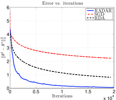
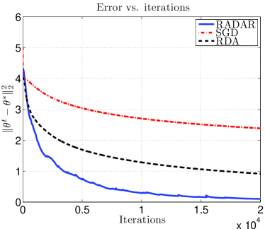
$d=20000$		$d=40000$

Figure 1: A comparison of RADAR with the RDA and SGD algorithms for $d=20000$ (left) and $d=40000$ (right). We plot $\|\theta^{t}-\theta^{*}\|_{2}^{2}$ averaged over 5 random trials versus the number of iterations.

Our second set of results provides comparisons to algorithms that are tailored to exploit sparsity. Our first baseline here is the approach that we described in our remarks following Theorem 1. In this approach, we use the same multi-step strategy as Algorithm 1 but keep $\lambda$ fixed. We refer to this as Epoch Dual Averaging (henceforth EDA), and again employ $\lambda=4\eta\sqrt{(\log d)/T}$ with this strategy. To maintain a fair comparison with the RADAR algorithm, our epochs are again terminated by halving of the squared $\ell_{p}$-error measured relative to $\theta^{*}$. Finally, we also evaluate the version of our algorithm with constant epoch lengths, as analyzed in Theorem 3 using epochs of length $\log(T)$, and henceforth referred to as RADAR-CONST. As shown in Figure 2, the RADAR-CONST has relatively large error during the initial epochs, before converging quite rapidly, a phenomenon consistent with our theory. Even though the RADAR-CONST method does not use the knowledge of $\theta^{*}$ to set epochs, all three methods exhibit the same eventual convergence rates, with RADAR (set with optimal epoch lengths) performing the best. Although RADAR-CONST is very slow in initial iterations, its convergence rate remains competitive with EDA (even though EDA does exploit knowledge of $\theta^{*}$), but is worse than RADAR as expected.

Overall, our experiments demonstrate that RADAR and RADAR-CONST have practical performance consistent with our theoretical predictions. Although optimal epoch length setting is not too critical for our approach, better data-dependent empirical rules for determining epoch lengths remains an interesting question for future research. The relatively poorer performance of EDA demonstrates the importance of our decreasing regularization schedule.

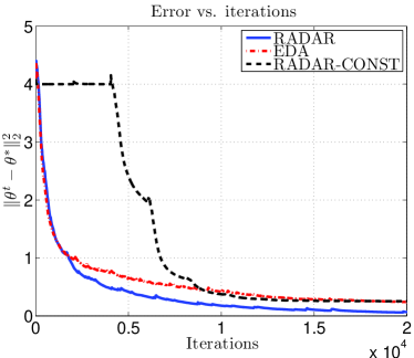
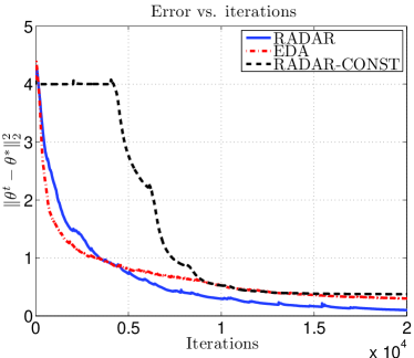
$d=20000$		$d=40000$

Figure 2: A comparison of RADAR with EDA and RADAR-CONST for $d=20000$ (left) and $d=40000$ (right). We plot $\|\theta^{t}-\theta^{*}\|_{2}^{2}$ averaged over 5 random trials versus the number of iterations.

6 Discussion

In this paper, we presented an algorithm that is able to take advantage of the strong convexity and sparsity conditions that are satsified by many common problems in machine learning. Our algorithm is simple and efficient to implement, and for a $d$-dimensional objective with an $s$-sparse optima, it achieves the minimax-optimal convergence rate $\mathcal{O}(s\log d/T)$. We also demonstrate optimal convergence rates for problems that have weakly sparse optima, with implications for problems such as sparse linear regression and sparse logistic regression. While we focus our attention exclusively on sparse vector recovery due to space constraints, the ideas naturally extend to other structures such as group sparse vectors and low-rank matrices [18]. It would be interest to study similar developments for other algorithms such as mirror descent or Nesterov’s accelerated gradient methods, leading to multi-step variants of those methods with optimal convergence rates in our setting.

Acknowledgements

The work of all three authors was partially supported by ONR MURI grant N00014-11-1-0688 to MJW. In addition, AA was partially supported by a Google Fellowship, and SN was partially supported by the Yahoo KSC award.

Appendix A Closed-form updates

In this appendix, we derive a closed form expression for the update (5b) when $\Omega=\mathbb{R}^{d}$. Recalling our definition of the prox-function (6), the constraint $\theta^{t+1}\in\Omega(R_{i})$ can be rewritten as $\psi_{y_{i},R_{i}}(\theta)\leq 2(p-1)$. We now form the Lagrangian at iteration $t+1$

$$\alpha^{t+1}\langle\mu^{t+1},\theta\rangle+\psi_{y_{i},R_{i}}(\theta)+\xi(\psi_{y_{i},R_{i}}(\theta)-2(p-1)),$$

where $\xi\geq 0$ is the Lagrangian parameter. The first-order optimality condition for the Lagrangian allows us to conclude that $\alpha^{t+1}\mu^{t+1}+\nabla\psi_{y_{i},R_{i}}(\theta^{t+1})(1+\xi)=0$, so that the iterate at time $t+1$ is given by

$$\theta^{t+1}=\nabla\psi^{*}_{y_{i},R_{i}}\left(-\frac{\alpha^{t+1}\mu^{t+1}}{1+\xi}\right),$$

where $\psi_{y_{i},R_{i}}^{*}(\mu)$ denotes the Fenchel conjugate [13]. Recalling the form of our prox-function, we have

$$\psi_{y_{i},R_{i}}(\theta)=\frac{1}{2(p-1)R_{1}^{2}}\|\theta-y_{i}\|_{p}^{2}\quad\mbox{and}\quad\psi_{y_{i},R_{i}}^{*}(\mu)=\langle y_{i},\mu\rangle+\frac{(p-1)R_{i}^{2}}{2}\|\mu\|_{q}^{2},$$

where $q=p/(p-1)$ is the conjugate exponent to $p$. This is a straightforward consequence of the Fenchel duality of $\ell_{p}$ norms (e.g., see Example 6.0.2  [13]).

We can now take the gradient of the dual function to obtain the following closed form expression

$$\theta^{t+1}=y_{i}+\frac{R_{i}^{2}(p-1)\alpha^{t+1}}{(1+\xi)}|\mu^{t+1}|^{(q-1)}\mbox{sign}(\mu^{t+1})\|\mu^{t+1}\|_{q}^{(2-q)}.$$

The value of $\xi$ can now be obtained by backsubstitution in the constraint $\theta\in\Omega(R_{i})$. Doing so and performing some algebra yields

$$\xi:=\max\left\{0,(p-1)\alpha^{t+1}\|\mu^{t+1}\|_{q}R_{i}-1\right\},$$

where $|\mu^{t+1}|^{(q-1)}$ refers to taking the absolute values and exponents elementwise and $q=p/(p-1)$ is the conjugate exponent to $p$.

Appendix B Proofs for convergence within a single epoch

In this appendix, we prove various results on convergence behavior within a single epoch, including Lemmas 1 and 2 as well as Proposition 1.

B.1 Proof of Lemma 1

By the optimality of $\widehat{\theta}_{i}$, we have

$$\makebox[0.0pt][l]{\hskip 2.05pt\rule[8.12498pt]{3.98999pt}{0.43057pt}}{\mathcal{L}}(\widehat{\theta}_{i})+\lambda_{i}\|\widehat{\theta}_{i}\|_{1} \leq\makebox[0.0pt][l]{\hskip 2.05pt\rule[8.12498pt]{3.98999pt}{0.43057pt}}{\mathcal{L}}(\theta^{*})+\lambda_{i}\|\theta^{*}\|_{1}.$$ (48)

From the local RSC assumption (28), for any vector $\theta$ feasible during epoch $i$, we have the lower bound

$$\makebox[0.0pt][l]{\hskip 2.05pt\rule[8.12498pt]{3.98999pt}{0.43057pt}}{\mathcal{L}}(\theta) \geq\makebox[0.0pt][l]{\hskip 2.05pt\rule[8.12498pt]{3.98999pt}{0.43057pt}}{\mathcal{L}}(\theta^{*})+\langle\nabla\makebox[0.0pt][l]{\hskip 2.05pt\rule[8.12498pt]{3.98999pt}{0.43057pt}}{\mathcal{L}}(\theta^{*}),\theta-\theta^{*}\rangle+\frac{\gamma}{2}\|\theta-\theta^{*}\|_{2}^{2}-\tau\|\theta-\theta^{*}\|_{1}^{2}$$

$$\stackrel{{\scriptstyle(i)}}{{\geq}}\makebox[0.0pt][l]{\hskip 2.05pt\rule[8.12498pt]{3.98999pt}{0.43057pt}}{\mathcal{L}}(\theta^{*})+\frac{\gamma}{2}\|\theta-\theta^{*}\|_{2}^{2}-\tau\|\theta-\theta^{*}\|_{1}^{2},$$ (49)

where step (i) follows since $\theta^{*}$ minimizes $\makebox[0.0pt][l]{\hskip 2.05pt\rule[8.12498pt]{3.98999pt}{0.43057pt}}{\mathcal{L}}(\theta)$. Applying inequality (49) with $\theta=\widehat{\theta}_{i}$ and combining with the initial bound (48) yields

$$\makebox[0.0pt][l]{\hskip 2.05pt\rule[8.12498pt]{3.98999pt}{0.43057pt}}{\mathcal{L}}(\widehat{\theta}_{i})+\lambda_{i}\|\widehat{\theta}_{i}\|_{1} \leq\makebox[0.0pt][l]{\hskip 2.05pt\rule[8.12498pt]{3.98999pt}{0.43057pt}}{\mathcal{L}}(\widehat{\theta}_{i})-\frac{\gamma}{2}\|\widehat{\theta}_{i}-\theta^{*}\|_{2}^{2}+\tau\|\widehat{\theta}_{i}-\theta^{*}\|_{1}^{2}+\lambda_{i}\|\theta^{*}\|_{1}.$$

Using the definition $\theta^{*}=\widehat{\theta}_{i}+\Delta_{i}$ and triangle inequality, we can further simplify to obtain

$$\lambda_{i}\|\widehat{\theta}_{i}\|_{1} \leq\lambda_{i}\|\theta^{*}\|_{1}-\frac{\gamma}{2}\|\theta^{*}-\widehat{\theta}_{i}\|_{2}^{2}+\tau\|\widehat{\theta}_{i}-\theta^{*}\|_{1}^{2}\;\leq\;\lambda_{i}\|\widehat{\theta}_{i}\|_{1}+\lambda_{i}\|\Delta_{i}\|_{1}-\frac{\gamma}{2}\|\Delta_{i}\|_{2}^{2}+\tau\|\Delta_{i}\|_{1}^{2},$$

Rearranging the terms above yields

$$\frac{\gamma}{2}\|\Delta_{i}\|_{2}^{2} \leq\lambda_{i}\|\Delta_{i}\|_{1}+\tau\|\Delta_{i}\|_{1}^{2}\leq 2\sqrt{s}\lambda_{i}\|\Delta_{i}\|_{2}+2\lambda_{i}\|\theta^{*}_{S^{c}}\|_{1}+8s\tau\|\Delta_{i}\|_{2}^{2}+8\tau\|\theta^{*}_{S^{c}}\|_{1}^{2}.$$

Some elementary algebra then yields that $\epsilon:=\|\Delta_{i}\|_{2}$ satisfies the quadratic inequality

$$\frac{1}{2}\big{\{}\gamma-16s\tau\big{\}}\epsilon^{2}-\big{\{}2\sqrt{s}\lambda_{i}\big{\}}\epsilon-\big{\{}2\lambda_{i}\|\theta^{*}_{S^{c}}\|_{1}+8\tau\|\theta^{*}_{S^{c}}\|_{1}^{2}\big{\}} \leq 0,$$

which then implies the $\ell_{2}$-error bound (38a).

In order to establish the $\ell_{1}$-error bound (38b), we require an auxiliary lemma that allows us to translate between the $\ell_{2}$ and $\ell_{1}$-norms:

Lemma 6.

For any pair of vectors $\theta,\tilde{\theta}\in\Omega$, suppose that $\|\tilde{\theta}\|_{1}\leq\|\theta\|_{1}+\epsilon$ for some $\epsilon\geq 0$. Then for any set $A\subseteq\{1,2,\ldots,d\}$, the vector $\Delta:=\theta-\tilde{\theta}$ satisfies the inequality

$$\|\Delta_{A^{c}}\|_{1}\leq \|\Delta_{A}\|_{1}+2\|\theta_{A^{c}}\|_{1}+\epsilon.$$ (50)

Proof.

Since $A$ and $A^{c}$ are disjoint, the bound assumed in the lemma statement can be written

$$\|\tilde{\theta}_{A}\|_{1}+\|\tilde{\theta}_{A^{c}}\|_{1}\leq\|\theta_{A}\|_{1}+\|\theta_{A^{c}}\|_{1}+\epsilon.$$ (51)

Since $\tilde{\theta}=\Delta+\theta$ by definition, triangle inequality implies that

$$\|\tilde{\theta}_{A}\|_{1}\geq\|\theta_{A}\|_{1}-\|\Delta_{A}\|_{1}\quad\mbox{and}\quad\|\tilde{\theta}_{A^{c}}\|_{1}\geq\|\Delta_{A^{c}}\|_{1}-\|\theta_{A^{c}}\|_{1}.$$

Substituting into the bound (51), we obtain

$$\|\Delta_{A^{c}}\|_{1}-\|\theta_{A^{c}}\|+\|\theta_{A}\|_{1}-\|\Delta_{A}\|_{1}\leq\|\theta_{A}\|_{1}+\|\theta_{A^{c}}\|_{1}+\epsilon,$$

and rearranging terms completes the proof. ∎

In particular, applying Lemma 6 to the pair $\theta=\widehat{\theta}_{i}$, and $\tilde{\theta}=\theta^{*}$ with the tolerance $\epsilon=0$ and the subset $A=S$, we find that the error vector $\Delta_{i}:=\widehat{\theta}_{i}-\theta^{*}$ satisfies the bounds

$$\|(\Delta_{i})_{S^{c}}\|_{1} \leq\|(\Delta_{i})_{S}\|_{1}+2\|\theta^{*}_{S^{c}}\|_{1}.$$ (52)

Consequently, we have

$$\|\Delta_{i}\|_{1} =\|(\Delta_{i})_{S}\|+\|(\Delta_{i})_{S^{c}}\|_{1}\;\leq\;2\|(\Delta_{i})_{S}\|_{1}+2\|\theta^{*}_{S^{c}}\|_{1}\;\leq\;2\sqrt{s}\|(\Delta_{i})_{S}\|_{2}+2\|\theta^{*}_{S^{c}}\|_{1},$$ (53)

where the final step uses the fact that $(\Delta_{i})_{S}$ is an $s$-vector.

B.2 Proof of Proposition 1: Inequality (36a)

We are now equipped to prove Proposition 1, beginning with the first bound (36a). Introducing the convenient shorthand $e^{t}=g^{t}-\nabla\makebox[0.0pt][l]{\hskip 2.05pt\rule[8.12498pt]{3.98999pt}{0.43057pt}}{\mathcal{L}}(\theta^{t})$, our assumptions guarantee that there are constants $G_{i}$ and $\sigma_{i}$ such that $\mathbb{E}\exp\left(\frac{\|e^{t}\|_{\infty}^{2}}{\sigma_{i}^{2}}\right)\leq\exp(1)$, and

$$|\makebox[0.0pt][l]{\hskip 2.05pt\rule[8.12498pt]{3.98999pt}{0.43057pt}}{\mathcal{L}}(\theta)-\makebox[0.0pt][l]{\hskip 2.05pt\rule[8.12498pt]{3.98999pt}{0.43057pt}}{\mathcal{L}}(\tilde{\theta})| \leq G_{i}\|\theta-\tilde{\theta}\|_{1}\quad\mbox{for all $\theta,\tilde{\theta}$ satisfying $\|\theta-y_{i}\|_{1}\leq R_{i}$.}$$ (54)

Our starting point is a known result for the convergence of the stochastic dual averaging algorithm. Recalling the definition $\bar{\theta}(T)=\sum_{t=1}^{T}\theta^{t}/T$, and letting ${\widehat{g}}^{t}=g^{t}+\lambda_{i}\nu^{t}$ be the stochastic subgradient at iteration $t$, we have

$$f_{i}(\bar{\theta}(T))-f_{i}(\widehat{\theta}_{i}) \leq\frac{1}{2T}\sum_{t=1}^{T}\frac{\alpha^{t-1}}{\gamma_{\psi}}\|{\widehat{g}}^{t}\|_{\infty}^{2}+\frac{1}{T\alpha^{T}}\psi_{y_{i},R_{i}}(\widehat{\theta}_{i})-\frac{1}{T}\sum_{t=1}^{T}\langle e^{t},\theta^{t}-\widehat{\theta}_{i}\rangle,$$ (55)

where $\gamma_{\psi}$ is the strong convexity coefficient of the prox-function with respect to the $\ell_{\infty}$ norm, equal to $1/(eR_{i}^{2})$ in our case. This bound follows directly from the analysis of Nesterov [22] and Xiao [30]; the specific form (55) given here corresponds to Lemma 2 of Duchi et al. [8].

Now observe that since ${\widehat{g}}^{t}=\nabla\makebox[0.0pt][l]{\hskip 2.05pt\rule[8.12498pt]{3.98999pt}{0.43057pt}}{\mathcal{L}}(\theta^{t})+\lambda_{i}\nu^{t}+e^{t}$, triangle inequality yields the upper bound

$$\|{\widehat{g}}^{t}\|_{\infty}^{2} \leq 2\big{(}\|\nabla\makebox[0.0pt][l]{\hskip 2.05pt\rule[8.12498pt]{3.98999pt}{0.43057pt}}{\mathcal{L}}(\theta^{t})+\lambda_{i}\nu^{t}\|_{\infty}^{2}+\|e^{t}\|_{\infty}^{2}\big{)}\;\stackrel{{\scriptstyle(i)}}{{\leq}}\;4G_{i}^{2}+4\lambda_{i}^{2}+2\|e^{t}\|_{\infty}^{2},$$

where inequality (i) uses the Lipschitz condition in Assumption 1, and the Lipschitz property of the $\ell_{1}$-norm. From this point, further simplifying the error bound (54) requires controlling the random terms

$$\sum_{t=1}^{T}\alpha^{t-1}\|e^{t}\|_{\infty}^{2}\quad\mbox{and}\quad\sum_{t=1}^{T}\langle e^{t},\theta^{t}-\widehat{\theta}_{i}\rangle$$ (56)

Accordingly, we state an auxiliary lemma that provide tail bounds appropriate for this purpose.

Lemma 7.

Under the sub-Gaussian tail condition (Assumption 3):

1. With step sizes $\alpha^{t}=\alpha/\sqrt{t}$, we have

   $$\sum_{t=1}^{T}\alpha^{t-1}\|e^{t}\|_{\infty}^{2}\leq 2\sigma^{2}_{i}\alpha\sqrt{T}+\sigma^{2}_{i}\omega\alpha\sqrt{2\log T}$$ (57)

   with probability at least $1-2\exp(-\omega^{2}/12)$ for all $\omega\leq 9\sqrt{\log T}$.

2. We have $\sum_{t=1}^{T}\langle e^{t},\,\widehat{\theta}_{i}-\theta^{t}\rangle\leq\omega R_{i}\sigma_{i}\sqrt{T}$ with probability at least $1-2\exp(-\omega^{2}/12)$.

See Appendix B.5 for the proof of this result. We now use it to control the terms in equation (56). Starting with the first term, we observe from Lemma 7 (a) that for $T\geq 1$, we are guaranteed that

$$\sum_{t=1}^{T}\alpha^{t-1}\|{\widehat{g}}^{t}\|_{\infty}^{2} \leq\sum_{t=1}^{T}\alpha^{t-1}(4G_{i}^{2}+4\lambda_{i}^{2}+2\|e^{t}\|_{\infty}^{2})$$

$$\leq 4(G_{i}^{2}+\lambda_{i}^{2})\sum_{t=1}^{T}\alpha^{t-1}+2\sigma_{i}^{2}\alpha(2\sqrt{T}+\omega_{i}\sqrt{\log T})$$

$$\leq 8(G_{i}^{2}+\lambda_{i}^{2})\alpha\sqrt{T}+22\sigma_{i}^{2}\alpha\sqrt{T},$$

with probability at least $1-2\exp(-\omega_{i}^{2}/12)$. Here the last step uses the inequality $9\log T\leq\sqrt{T}$ valid for all $T\geq 1$, as well as the assumption $\omega_{i}\leq 9\sqrt{\log T}$. Thus, we have established an upper bound on the gradient terms with an effective Lipschitz constant

$$\sum_{t=1}^{T}\alpha^{t-1}\|{\widehat{g}}^{t}\|_{\infty}^{2}\leq 22\alpha\sqrt{T}(G_{i}^{2}+\lambda_{i}^{2}+\sigma_{i}^{2}).$$ (58)

Part (b) of Lemma 7 directly controls the second random quantity.

We now plug in the results of these lemmas into our earlier error bound (55), which yields, with probability at least $1-3\exp(-\omega_{i}^{2}/12)$, the upper bound

$$f_{i}(\bar{\theta}(T))-f_{i}(\widehat{\theta}_{i}) \leq\frac{22\alpha}{2\gamma_{\psi}\sqrt{T}}(G_{i}^{2}+\lambda_{i}^{2}+\sigma_{i}^{2})+\frac{A_{\psi}}{\alpha\sqrt{T}}+\frac{\omega_{i}\sigma_{i}R_{i}}{\sqrt{T}}$$

$$\leq 10\sqrt{G_{i}^{2}+\sigma_{i}^{2}+\lambda_{i}^{2}}\sqrt{\frac{A_{\psi}}{\gamma_{\psi}T}}+\frac{\omega_{i}\sigma_{i}R_{i}}{\sqrt{T}}.$$

Here the second inequality uses the setting $\alpha=5\sqrt{A_{\psi}\gamma_{\psi}/(G_{i}^{2}+\lambda_{i}^{2}+\sigma_{i}^{2})}$. We also note that under our assumption that $\psi$ is $1$-strongly convex with respect to $\|\cdot\|_{1}$, we have that $\gamma_{\psi}=1/(eR_{i}^{2})$ at epoch $i$. Thus with probability at least $1-3\exp(-\omega_{i}^{2}/12)$, we have the error bound

$$f_{i}(\bar{\theta}(T))-f_{i}(\widehat{\theta}_{i}) \leq 30R_{i}\sqrt{\frac{A_{\psi}(G_{i}^{2}+\sigma_{i}^{2}+\lambda_{i}^{2})}{T}}+\frac{\omega_{i}\sigma_{i}R_{i}}{\sqrt{T}}$$

$$\leq 30R_{i}\sqrt{\frac{A_{\psi}(G_{i}^{2}+\sigma_{i}^{2})}{T}}+30R_{i}\lambda_{i}\sqrt{\frac{A_{\psi}}{T}}+\frac{\omega_{i}\sigma_{i}R_{i}}{\sqrt{T}},$$ (59)

thus completing the first bound in Proposition 1.

B.3 Proof of Lemma 2

The main idea of this proof is to first convert the error bound (B.2) from function values into $\ell_{1}$ and $\ell_{2}$-norm bounds by exploiting the (approximate) sparsity of $\theta^{*}$. We will then use these bounds to simplify the RSC condition. Since the error bound (B.2) for the minimizer $\widehat{\theta}_{i}$, it also holds for any other feasible vector. In particular, applying it to $\theta^{*}$, we obtain the bound

$$f_{i}(\bar{\theta}(T_{i}))-f_{i}(\theta^{*}) \leq c\,\frac{30R_{i}}{\lambda_{i}}\sqrt{\frac{A_{\psi}(G_{i}^{2}+\sigma_{i}^{2})}{T_{i}}}+30R_{i}\sqrt{\frac{A_{\psi}}{T_{i}}}+\frac{\omega_{i}\sigma_{i}R_{i}}{\lambda_{i}\sqrt{T_{i}}}.$$ (60)

Our next step is to lower bound the left-hand side of this inequality. We have

$$f_{i}(\bar{\theta}(T_{i}))-f_{i}(\theta^{*}) =\makebox[0.0pt][l]{\hskip 2.05pt\rule[8.12498pt]{3.98999pt}{0.43057pt}}{\mathcal{L}}(\bar{\theta}(T_{i}))+\lambda_{i}\|\bar{\theta}(T_{i})\|_{1}-\makebox[0.0pt][l]{\hskip 2.05pt\rule[8.12498pt]{3.98999pt}{0.43057pt}}{\mathcal{L}}(\theta^{*})-\lambda_{i}\|\theta^{*}\|_{1}$$

$$\stackrel{{\scriptstyle(i)}}{{\geq}}\makebox[0.0pt][l]{\hskip 2.05pt\rule[8.12498pt]{3.98999pt}{0.43057pt}}{\mathcal{L}}(\theta^{*})+\lambda_{i}\|\bar{\theta}(T_{i})\|_{1}-\makebox[0.0pt][l]{\hskip 2.05pt\rule[8.12498pt]{3.98999pt}{0.43057pt}}{\mathcal{L}}(\theta^{*})-\lambda_{i}\|\theta^{*}\|_{1}$$

$$=\lambda_{i}\big{\{}\|\bar{\theta}(T_{i})\|_{1}-\|\theta^{*}\|_{1}\big{\}},$$

where inequality (i) follows since $\theta^{*}$ minimizes $\makebox[0.0pt][l]{\hskip 2.05pt\rule[8.12498pt]{3.98999pt}{0.43057pt}}{\mathcal{L}}$. Combining with the bound (60) yields

$$\|\bar{\theta}(T_{i})\|_{1}\leq\|\theta^{*}\|_{1}+\frac{30R_{i}}{\lambda_{i}}\sqrt{\frac{A_{\psi}(G_{i}^{2}+\sigma_{i}^{2})}{T_{i}}}+30R_{i}\sqrt{\frac{A_{\psi}}{T_{i}}}+\frac{\omega_{i}\sigma_{i}R_{i}}{\lambda_{i}\sqrt{T_{i}}}.$$ (61)

At this point we recall the shorthand notations $\Delta^{*}(T_{i})=\bar{\theta}(T_{i})-\theta^{*}$ and $\widehat{\Delta}(T_{i})=\bar{\theta}(T_{i})-\widehat{\theta}_{i}$. In order to bring the above bound on $\|\bar{\theta}(T_{i})\|_{1}$ closer to the statement of the lemma, we can appeal to Lemma 6. Indeed an application of the lemma in conjunction with the inequality (61) results in the bound

$$\|\Delta^{*}(T_{i})_{S^{c}}\|_{1}\leq\|\Delta^{*}(T_{i})_{S}\|_{1}+\frac{30R_{i}}{\lambda_{i}}\sqrt{\frac{A_{\psi}(G_{i}^{2}+\sigma_{i}^{2})}{T_{i}}}+30R_{i}\sqrt{\frac{A_{\psi}}{T_{i}}}+\frac{\omega_{i}\sigma_{i}R_{i}}{\lambda_{i}\sqrt{T_{i}}}+2\|\theta^{*}_{S^{c}}\|_{1}.$$ (62)

Our next step is to convert the above cone bound on $\Delta^{*}(T_{i})$ into a similar result for $\widehat{\Delta}(T_{i})$. In order to do so, we observe that $\Delta^{*}(T_{i})-\widehat{\Delta}(T_{i})=\widehat{\theta}_{i}-\theta^{*}$, and hence

$$\|\widehat{\theta}_{i}-\theta^{*}\|_{1} =\|\Delta^{*}_{S}(T_{i})-\widehat{\Delta}_{S}(T_{i})\|_{1}+\|\Delta^{*}_{S^{c}}(T_{i})-\widehat{\Delta}_{S^{c}}(T_{i})\|_{1}$$

$$\geq\big{\{}\|\Delta^{*}_{S}(T_{i})\|_{1}-\|\widehat{\Delta}_{S}(T_{i})\|_{1}\big{\}}-\big{\{}\|\Delta^{*}_{S^{c}}(T_{i})\|_{1}-\|\widehat{\Delta}_{S^{c}}(T_{i})\|_{1}\big{\}},$$

and hence

$$\|\widehat{\Delta}_{S^{c}}(T_{i})\|_{1}-\|\widehat{\Delta}_{S}(T_{i})\|_{1}\leq\|\Delta^{*}_{S^{c}}(T_{i})\|_{1}-\|\Delta^{*}_{S}(T_{i})\|_{1}+\|\widehat{\theta}_{i}-\theta^{*}\|_{1}.$$

Consequently, Lemma 1 provides the final piece to complete the proof. Combining inequality (39) obtained from Lemma 1 with our earlier bound (62) yields

$$\|\widehat{\Delta}(T_{i})_{S^{c}}\|_{1}\leq\|\widehat{\Delta}(T_{i})_{S}\|_{1}+\frac{9s\lambda_{i}}{\overline{\gamma}}+\|\theta^{*}_{S^{c}}\|_{1}\left(6+8\sqrt{\frac{s\tau}{\overline{\gamma}}}\right)+\frac{30R_{i}}{\lambda_{i}}\sqrt{\frac{A_{\psi}(G_{i}^{2}+\sigma_{i}^{2})}{T_{i}}}+30R_{i}\sqrt{\frac{A_{\psi}}{T_{i}}}+\frac{\omega_{i}\sigma_{i}R_{i}}{\lambda_{i}\sqrt{T_{i}}}.$$

Consequently, a further use of the inequality $\|\widehat{\Delta}(T_{i})_{S}\|_{1}\leq\sqrt{s}\|\widehat{\Delta}(T_{i})\|_{2}$ allows us to conclude that there is a universal constant $c$ such that

$$\|\widehat{\Delta}\|_{1}^{2} \leq 8s\|\widehat{\Delta}\|_{2}^{2}+c\,\left(\frac{s^{2}\lambda_{i}^{2}}{\overline{\gamma}^{2}}+\frac{R_{i}^{2}}{\lambda_{i}^{2}T_{i}}\left(A_{\psi}(G_{i}^{2}+\sigma_{i}^{2})+\omega_{i}^{2}\sigma_{i}^{2}\right)+\frac{R_{i}^{2}A_{\psi}}{T_{i}}+\|\theta^{*}_{S^{c}}\|_{1}^{2}\left(1+\frac{s\tau}{\overline{\gamma}}\right)\right)$$ (63)

with probability at least $1-3\exp(-\omega_{i}^{2}/12)$. Substituting the settings (34) and (32) of $\lambda_{i}$ and $T_{i}$ respectively into the above bound yields

$$\|\widehat{\Delta}(T_{i})\|_{1}^{2} \leq 8s\|\widehat{\Delta}(T_{i})\|_{2}^{2}+c\,\left(R_{i}^{2}\frac{\overline{\gamma}}{\gamma}+s\varepsilon^{2}(\theta^{*};S,\tau)\right),$$ (64)

where we recall the notation $\varepsilon^{2}(\theta^{*};S,\tau)=\frac{\|\theta^{*}_{S^{c}}\|_{1}^{2}}{s}\big{(}1+\frac{s\tau}{\overline{\gamma}}\big{)}$.

In order to complete the proof, we now invoke the RSC assumption applied to the function $f_{i}$. Specifically, since $\widehat{\theta}_{i}$ minimizes $f_{i}$, the RSC condition implies that

$$\frac{\gamma}{2}\|\widehat{\Delta}(T_{i})\|_{2}^{2}\leq f_{i}(\bar{\theta}(T_{i}))-f_{i}(\widehat{\theta}_{i})+\tau\|\widehat{\Delta}(T_{i})\|_{1}^{2}.$$

Combining the above inequality with the bound (64) yields

$$\frac{\gamma}{2}\|\widehat{\Delta}(T_{i})\|_{2}^{2}\leq f_{i}(\bar{\theta}(T_{i}))-f_{i}(\widehat{\theta}_{i})+\tau\left[8s\|\widehat{\Delta}(T_{i})\|_{2}^{2}+c\,\left(R_{i}^{2}\frac{\overline{\gamma}}{\gamma}+s\varepsilon^{2}(\theta^{*};S,\tau)\right)\right].$$

Rearranging terms and recalling the notation $\overline{\gamma}=\gamma-16s\tau$ completes the proof.

B.4 Proof of Proposition 1: Inequality (36b)

Equipped with Lemma 2, we are now ready to prove the second part of Proposition 1. In particular, using the inequality (63) in the proof of Lemma 2, we observe that with probability at least $1-3\exp(-\omega_{i}^{2}/12)$, we have

$$\|\widehat{\Delta}\|_{1}^{2} \leq 8s\|\widehat{\Delta}\|_{2}^{2}+c\,\left(\frac{s^{2}\lambda_{i}^{2}}{\overline{\gamma}^{2}}+\frac{R_{i}^{2}}{\lambda_{i}^{2}T_{i}}\left(A_{\psi}(G_{i}^{2}+\sigma_{i}^{2})+\omega_{i}^{2}\sigma_{i}^{2}\right)+\frac{R_{i}^{2}A_{\psi}}{T_{i}}+s\varepsilon^{2}(\theta^{*};S,\tau)\right)$$

$$\leq\frac{16s}{\gamma}(f_{i}(\bar{\theta}(T_{i}))-f_{i}(\widehat{\theta}_{i})+\tau\|\widehat{\Delta}\|_{1}^{2})+c\,\left(\frac{s^{2}\lambda_{i}^{2}}{\overline{\gamma}^{2}}+\frac{R_{i}^{2}}{\lambda_{i}^{2}T_{i}}\left(A_{\psi}(G_{i}^{2}+\sigma_{i}^{2})+\omega_{i}^{2}\sigma_{i}^{2}\right)+\frac{R_{i}^{2}A_{\psi}}{T_{i}}+s\varepsilon^{2}(\theta^{*};S,\tau)\right).$$

Here the second inequality uses the local RSC condition (28), and the fact that $\widehat{\theta}_{i}$ minimizes $f_{i}$.

From hereonwards, all our inequalities hold with probability at least $1-3\exp(-\omega_{i}^{2}/12)$, so that we no longer state it explicitly. Rearranging terms and recalling the definition (30) of $\overline{\gamma}$, we obtain that

$$\frac{\overline{\gamma}}{\gamma}\|\widehat{\Delta}\|_{1}^{2} \leq\frac{16s}{\overline{\gamma}}\,(f_{i}(\bar{\theta}(T_{i}))-f_{i}(\widehat{\theta}_{i}))+c\,\left(\frac{s^{2}\lambda_{i}^{2}}{\overline{\gamma}^{2}}+\frac{R_{i}^{2}}{\lambda_{i}^{2}T_{i}}\left(A_{\psi}(G_{i}^{2}+\sigma_{i}^{2})+\omega_{i}^{2}\sigma_{i}^{2}\right)+\frac{R_{i}^{2}A_{\psi}}{T_{i}}+s\varepsilon^{2}(\theta^{*};S,\tau)\right).$$

Combining the above bound with our earlier inequality (B.2) yields $\frac{\overline{\gamma}}{\gamma}\|\widehat{\Delta}\|_{1}^{2}\leq\Phi_{1}+\Phi_{2}$, where

$$\Phi_{1} :=\frac{16sR_{i}}{\overline{\gamma}\sqrt{T_{i}}}\left(4\sqrt{A_{\psi}(G_{i}^{2}+\sigma_{i}^{2})}+4\lambda_{i}\sqrt{A_{\psi}}+\omega_{i}\sigma_{i}\right),\quad\mbox{and}$$ (65a)

$$\Phi_{2} :=c\,\left(\frac{s^{2}\lambda_{i}^{2}}{\overline{\gamma}^{2}}+\frac{R_{i}^{2}}{\lambda_{i}^{2}T_{i}}\left(A_{\psi}(G_{i}^{2}+\sigma_{i}^{2})+\omega_{i}^{2}\sigma_{i}^{2}\right)+\frac{R_{i}^{2}A_{\psi}}{T_{i}}+s\varepsilon^{2}(\theta^{*};S,\tau)\right)$$ (65b)

By the Cauchy-Schwartz inequality, we have $\frac{sR_{i}\lambda_{i}}{\overline{\gamma}}\sqrt{\frac{A_{\psi}}{T_{i}}}\leq 2\frac{s^{2}\lambda_{i}^{2}}{\overline{\gamma}^{2}}+2\frac{R_{i}^{2}A_{\psi}}{T_{i}}$, and hence

$$\Phi_{1} \leq\frac{16sR_{i}}{\overline{\gamma}\sqrt{T_{i}}}\left(4\sqrt{A_{\psi}(G_{i}^{2}+\sigma_{i}^{2})}+\omega_{i}\sigma_{i}\right)+128\left(\frac{s^{2}\lambda_{i}^{2}}{\overline{\gamma}^{2}}+\frac{R_{i}^{2}A_{\psi}}{T_{i}}+\right).$$ (66)

Noting that $\Phi_{1}$ and $\Phi_{2}$ involve multiple terms, some increasing and others decreasing in $\lambda_{i}$, we optimize the choice of $\lambda_{i}$, in particular by setting

$$\lambda_{i}^{2} =\frac{R_{i}\overline{\gamma}}{s\sqrt{T_{i}}}\sqrt{A_{\psi}(G_{i}^{2}+\sigma_{i}^{2})+\omega_{i}^{2}\sigma_{i}^{2}}.$$ (67)

Using this setting and combining the upper bound $\frac{\overline{\gamma}}{\gamma}\|\widehat{\Delta}\|_{1}^{2}\leq\Phi_{1}+\Phi_{2}$ with the form (65b) of $\Phi_{2}$ and the upper bound (66) on $\Phi_{1}$, we find that

$$\|\widehat{\Delta}\|_{1}^{2} \leq c\,\frac{\gamma}{\overline{\gamma}}\left[\frac{sR_{i}}{\overline{\gamma}\sqrt{T_{i}}}\left(\sqrt{A_{\psi}(G_{i}^{2}+\sigma_{i}^{2})}+\omega_{i}\sigma_{i}\right)+\frac{R_{i}^{2}A_{\psi}}{T_{i}}+s\varepsilon^{2}(\theta^{*};S,\tau)\right].$$ (68)

Combining the above inequality with the error bound (39) for $\widehat{\theta}_{i}$ and triangle inequality leads to

$$\|\Delta^{*}\|_{1}^{2} \leq 2\|\widehat{\Delta}\|_{1}^{2}+2\|\theta^{*}-\widehat{\theta}_{i}\|_{1}^{2}\leq 2\|\widehat{\Delta}\|_{1}^{2}+\frac{162s^{2}\lambda_{i}^{2}}{\overline{\gamma}^{2}}+c\,s\;\varepsilon^{2}(\theta^{*};S,\tau)$$

$$\leq 2\|\widehat{\Delta}\|_{1}^{2}+\frac{\gamma}{\overline{\gamma}}c\left(\frac{s^{2}\lambda_{i}^{2}}{\overline{\gamma}^{2}}+\,s\;\varepsilon^{2}(\theta^{*};S,\tau)\right),$$

where the second inequality follows since $\gamma\geq\overline{\gamma}$. Substituting the setting (67) of $\lambda_{i}$ yields an upper bound identical to our earlier bound (68) with different constants.

Finally, in order to use $\bar{\theta}(T_{i})$ as our next prox-center $y_{i+1}$, we would also like to control the error $\|\bar{\theta}(T_{i})-\widehat{\theta}_{i+1}\|_{1}^{2}$. Since $\lambda_{i+1}\leq\lambda_{i}$ by assumption, we obtain the same form of error bound (68). We want to run the epoch till all these error terms drop to $R_{i+1}^{2}:=R_{i}^{2}/2$. Recalling our assumption that $\gamma\varepsilon^{2}(\theta^{*};S,\tau)/\overline{\gamma}\leq R_{i}^{2}/4$, it suffices to set the epoch length $T_{i}$ to ensure that

$$c\,\frac{sR_{i}\gamma}{\overline{\gamma}^{2}\sqrt{T_{i}}}\sqrt{A_{\psi}(G_{i}^{2}+\sigma_{i}^{2})}\leq\frac{R_{i}^{2}}{12},\qquad c\,\frac{sR_{i}\gamma}{\overline{\gamma}^{2}\sqrt{T_{i}}}\omega_{i}\sigma_{i}\leq\frac{R_{i}^{2}}{12},\quad\mbox{and}\quad c\,\frac{\gamma R_{i}^{2}A_{\psi}}{\overline{\gamma}T_{i}}\leq\frac{R_{i}^{2}}{12}.$$

All the above conditions are met if we choose the epoch length

$$T_{i} =C\,\left[\frac{s^{2}\gamma^{2}}{\overline{\gamma}^{4}R_{i}^{2}}\left(A_{\psi}(G_{i}^{2}+\sigma_{i}^{2})+\omega_{i}^{2}\sigma_{i}^{2}\right)+\frac{A_{\psi}\gamma}{\overline{\gamma}}\right],$$

for a suitably large universal constant $C$, which completes the proof of the second part of the proposition. The stated bound in function values follows from substituting the choice of $\lambda_{i}$ in our earlier bound (B.2) and some straightforward algebra.

B.5 Proof of Lemma 7

It remains to prove Lemma 7, a result used during the proof of Proposition 1. We do so by exploiting some classical martingale tail bounds of the Azuma-Hoeffding type. The particular result given here is due to Lan et al. [16]:

Lemma 8.

Let $z_{1},z_{2},\ldots$ be a sequence of i.i.d. random variables, let $\sigma_{t}>0$, $t=1,2,\ldots$ be a sequence of deterministic numbers, and let $\phi_{t}=\phi_{t}(z^{t})$ be deterministic (measurable) functions of $z^{t}=(z_{1},z_{2},\ldots,z_{t})$. Using $\mathcal{F}_{t}$ to denote the $\sigma$-field of $z^{t}$, we have:

• Suppose $\mathbb{E}[\phi_{t}\,\mid\mathcal{F}_{t-1}]=0$ with probability one and $\mathbb{E}[\exp(\phi_{t}^{2}/\sigma_{t}^{2})\,\mid\mathcal{F}_{t-1}]\leq\exp(1)$ with probability one for all $t$. Then

  $$\mathbb{P}\Big{[}\sum_{t=1}^{T}\phi_{t}>\delta\big{(}\sum_{t=1}^{T}\sigma_{t}^{2}\big{)}^{1/2}\Big{]} \leq\exp(-\delta^{2}/3)\qquad\mbox{for all $\delta\geq 0$.}$$ (69)

• Suppose that $\mathbb{E}[\exp(|\phi_{t}|/\sigma_{t})\,\mid\mathcal{F}_{t-1}]\leq\exp(1)$ w.p. 1 for $t$. Letting $\sigma^{T}=(\sigma_{1},\ldots,\sigma_{T})$, we have the bound

  $$\mathbb{P}\left[\sum_{t=1}^{T}\phi_{t}>\|\sigma^{T}\|_{1}+\delta\|\sigma^{T}\|_{2}\right] \leq\exp(-\delta^{2}/12)+\exp\left(-\frac{3\|\sigma^{T}\|_{2}}{4\|\sigma^{T}\|_{\infty}}\delta\right)$$

  $$\leq\exp(-\delta^{2}/12)+\exp(-3\delta/4).$$ (70)

We now use this lemma to prove parts (a) and (b) of Lemma 7.

B.5.1 Proof of part (a)

We start by showing that the conditions of Lemma 8 are satisfied. Indeed, by Assumption 3, we have

$$\mathbb{E}\exp\left(\frac{\alpha^{t-1}\|e^{t}\|_{\infty}^{2}}{\sigma_{i}^{2}\alpha^{t-1}}\right) =\mathbb{E}\exp\left(\frac{\|e^{t}\|_{\infty}^{2}}{\sigma_{i}^{2}}\right)\leq\exp(1).$$

Consequently, in order to satisfy the condition of Lemma 8(b), it suffices to set $\sigma_{t}=\sigma^{2}_{i}\alpha^{t-1}$. Recalling our choice $\alpha^{t}=\alpha/\sqrt{t}$, we find that

$$\|\sigma^{T}\|_{1} =\sigma_{i}^{2}\sum_{t=1}^{T}\alpha^{t}=\sigma_{i}^{2}\alpha\sum_{t=1}^{T}\frac{1}{\sqrt{t}}\leq 2\sigma_{i}^{2}\alpha\sqrt{T},$$

$$\|\sigma^{T}\|_{2} =\sigma_{i}^{2}\sqrt{\sum_{t=1}^{T}(\alpha^{t})^{2}}=\sigma_{i}^{2}\alpha\sqrt{\sum_{t=1}^{T}\frac{1}{t}}\leq\sigma_{i}^{2}\alpha\sqrt{2\log T}\quad\mbox{and}$$

$$\|\sigma^{T}\|_{\infty} =\sigma_{i}^{2}\alpha.$$

Plugging the above quantities in the statement of Lemma 8(b) with $\delta=\omega_{i}$ yields

$$\mathbb{P}\Big{[}\sum_{t=1}^{T}\alpha^{t-1}\|e^{t}\|_{\infty}^{2}>2\sigma_{i}^{2}\alpha\sqrt{T}+\omega_{i}\sigma^{2}_{i}\alpha\sqrt{2\log T}\Big{]} \leq\exp(-\omega_{i}^{2}/12)+\exp\left(-\frac{3\sigma_{i}^{2}\alpha\sqrt{\sum_{t=1}^{T}1/t}}{4\sigma_{i}^{2}\alpha}\omega_{i}\right)$$

$$\leq\exp(-\omega_{i}^{2}/12)+\exp\left(-\frac{3\sqrt{\log T}}{4}\omega_{i}\right)$$

$$\leq 2\exp(-\omega_{i}^{2}/12),$$

where the last inequality uses our assumption $\omega_{i}\leq 9\sqrt{\log T}$, thus completing the proof.

B.5.2 Proof of part (b)

We now turn to part (b) of Lemma 7. By assumption, we have $\mathbb{E}[e^{t}\mid\mathcal{F}_{t-1}]=0$; moreover, the random variable $\theta^{t}$ is measurable with respect to $\mathcal{F}_{t-1}$ and $\widehat{\theta}_{i}$ is deterministic. Consequently, the first condition of Lemma 8(a) is satisfied. For the second condition, we observe that by Hölder’s inequality and Assumption 3, we have

$$\mathbb{E}\exp\left(\frac{\langle e^{t},\theta^{t}-\widehat{\theta}_{i}\rangle^{2}}{4R_{i}^{2}\sigma_{i}^{2}}\right) \leq\mathbb{E}\exp\left(\frac{\|e^{t}\|_{\infty}^{2}\|\theta^{t}-\widehat{\theta}_{i}\|_{1}^{2}}{4R_{i}^{2}\sigma_{i}^{2}}\right)$$

$$\stackrel{{\scriptstyle(a)}}{{\leq}}\mathbb{E}\exp\left(\frac{4\|e^{t}\|_{\infty}^{2}R_{i}^{2}}{4R_{i}^{2}\sigma_{i}^{2}}\right)=\mathbb{E}\exp\left(\frac{\|e^{t}\|_{\infty}^{2}}{\sigma_{i}^{2}}\right)\leq\exp(1).$$

Here inequality (a) uses the facts that $\|\theta^{t}-y_{i}\|_{1}\leq R_{i}$ and $\|\widehat{\theta}_{i}-y_{i}\|_{1}\leq R_{i}$ by the definition of our updates (5), so that the conditions of Lemma 8(a) are satisfied with $\sigma_{t}=2\sigma_{i}R_{i}$. Plugging this setting in the result of the lemma and setting $\delta=\omega/2$ completes the proof.

Appendix C Proof of Lemma 3

The proof of this lemma is based on pair of auxiliary results, which we begin by stating.

Lemma 9.

Suppose at some epoch $k$, we have the bound $\|y_{k}-\theta^{*}\|_{1}\leq R_{k}$. Then for all epochs $j\geq k$, we have

$$\|y_{j}-\theta^{*}\|_{1}\leq 8R_{k}.$$

Lemma 10.

Under the conditions of Lemma 3, for any epoch $i>k$, we have

$$f_{i}(y_{i+1})-f_{i}(y_{i}) \leq c\,\frac{R_{k}^{2}\overline{\gamma}^{2}}{s\gamma}\,2^{-(i-k)/2}.$$ (71)

See Sections C.2 and C.3 for the proofs of these two lemmas, respectively.

C.1 Main argument

With these auxiliary results in hand, we now turn to the proof of Lemma 3. By the definition of $f_{i}$, we have

$$\makebox[0.0pt][l]{\hskip 2.05pt\rule[8.12498pt]{3.98999pt}{0.43057pt}}{\mathcal{L}}(y_{i+1})-\makebox[0.0pt][l]{\hskip 2.05pt\rule[8.12498pt]{3.98999pt}{0.43057pt}}{\mathcal{L}}(\theta^{*}) =(\makebox[0.0pt][l]{\hskip 2.05pt\rule[8.12498pt]{3.98999pt}{0.43057pt}}{\mathcal{L}}y_{i+1}-\makebox[0.0pt][l]{\hskip 2.05pt\rule[8.12498pt]{3.98999pt}{0.43057pt}}{\mathcal{L}}(y_{i}))+(\makebox[0.0pt][l]{\hskip 2.05pt\rule[8.12498pt]{3.98999pt}{0.43057pt}}{\mathcal{L}}(y_{i})-\makebox[0.0pt][l]{\hskip 2.05pt\rule[8.12498pt]{3.98999pt}{0.43057pt}}{\mathcal{L}}(\theta^{*}))$$

$$=(f_{i}(y_{i+1})-f_{i}(y_{i}))+\lambda_{k}(\|y_{i}\|_{1}-\|y_{i+1}\|_{1})+(\makebox[0.0pt][l]{\hskip 2.05pt\rule[8.12498pt]{3.98999pt}{0.43057pt}}{\mathcal{L}}(y_{i})-\makebox[0.0pt][l]{\hskip 2.05pt\rule[8.12498pt]{3.98999pt}{0.43057pt}}{\mathcal{L}}(\theta^{*}))$$

$$\stackrel{{\scriptstyle(i)}}{{\leq}}c\,\frac{R_{k}^{2}\overline{\gamma}^{2}}{s\gamma}\,2^{-(i-k)/2}+\lambda_{i}R_{i}+(\makebox[0.0pt][l]{\hskip 2.05pt\rule[8.12498pt]{3.98999pt}{0.43057pt}}{\mathcal{L}}(y_{i})-\makebox[0.0pt][l]{\hskip 2.05pt\rule[8.12498pt]{3.98999pt}{0.43057pt}}{\mathcal{L}}(\theta^{*})),$$

where step (i) follows from a combination of Lemma 10, and triangle inequality along with the feasibility of $y_{i+1}$ at epoch $i$ since $\|y_{i}\|_{1}-\|y_{i+1}\|_{1}\leq\|y_{i}-y_{i+1}\|_{1}\leq R_{i}$. By applying the Cauchy-Schwarz inequality to the second term in the bound above, we obtain

$$\makebox[0.0pt][l]{\hskip 2.05pt\rule[8.12498pt]{3.98999pt}{0.43057pt}}{\mathcal{L}}(y_{i+1})-\makebox[0.0pt][l]{\hskip 2.05pt\rule[8.12498pt]{3.98999pt}{0.43057pt}}{\mathcal{L}}(\theta^{*}) \leq c\,\frac{R_{{k^{*}}}^{2}2^{-(i-k)/2}\overline{\gamma}^{2}}{s\gamma}+\frac{\overline{\gamma}R_{i}^{2}}{2s}+\frac{s\lambda_{i}^{2}}{2\overline{\gamma}}+(\makebox[0.0pt][l]{\hskip 2.05pt\rule[8.12498pt]{3.98999pt}{0.43057pt}}{\mathcal{L}}(y_{i})-\makebox[0.0pt][l]{\hskip 2.05pt\rule[8.12498pt]{3.98999pt}{0.43057pt}}{\mathcal{L}}(\theta^{*}))$$

$$\leq c\,\frac{R_{{k^{*}}}^{2}2^{-(k-{k^{*}})/2}\gamma}{s}+(\makebox[0.0pt][l]{\hskip 2.05pt\rule[8.12498pt]{3.98999pt}{0.43057pt}}{\mathcal{L}}(y_{k})-\makebox[0.0pt][l]{\hskip 2.05pt\rule[8.12498pt]{3.98999pt}{0.43057pt}}{\mathcal{L}}(\theta^{*})),$$

where the last inequality uses the setting (15) of $\lambda_{i}$ and the setting (32) of $T_{i}$. Recursing the argument further yields

$$\makebox[0.0pt][l]{\hskip 2.05pt\rule[8.12498pt]{3.98999pt}{0.43057pt}}{\mathcal{L}}(y_{j})-\makebox[0.0pt][l]{\hskip 2.05pt\rule[8.12498pt]{3.98999pt}{0.43057pt}}{\mathcal{L}}(\theta^{*}) \leq c\,\sum_{i=k+1}^{j}\frac{R_{k}^{2}2^{-(i-k)/2}\overline{\gamma}^{2}}{s\gamma}+(\makebox[0.0pt][l]{\hskip 2.05pt\rule[8.12498pt]{3.98999pt}{0.43057pt}}{\mathcal{L}}(y_{k+1})-\makebox[0.0pt][l]{\hskip 2.05pt\rule[8.12498pt]{3.98999pt}{0.43057pt}}{\mathcal{L}}(\theta^{*}))$$

$$\leq c\frac{R_{k}^{2}\overline{\gamma}^{2}}{(\sqrt{2}-1)s\gamma}+(\makebox[0.0pt][l]{\hskip 2.05pt\rule[8.12498pt]{3.98999pt}{0.43057pt}}{\mathcal{L}}(y_{k+1})-\makebox[0.0pt][l]{\hskip 2.05pt\rule[8.12498pt]{3.98999pt}{0.43057pt}}{\mathcal{L}}(\theta^{*})),$$

where the second inequality upper bounds the sum of the geometric progression. Recalling the given conditions in the lemma, we obtain the upper bound

$$\makebox[0.0pt][l]{\hskip 2.05pt\rule[8.12498pt]{3.98999pt}{0.43057pt}}{\mathcal{L}}(y_{k+1})-\makebox[0.0pt][l]{\hskip 2.05pt\rule[8.12498pt]{3.98999pt}{0.43057pt}}{\mathcal{L}}(\theta^{*}) \leq f_{k}(y_{k+1})-f_{k}(\theta^{*})+2\lambda_{k}R_{k}\;\leq\;c\,\frac{\overline{\gamma}^{2}R_{k}^{2}}{s\gamma}.$$

Combining the two previous bounds yields $\makebox[0.0pt][l]{\hskip 2.05pt\rule[8.12498pt]{3.98999pt}{0.43057pt}}{\mathcal{L}}(y_{j})-\makebox[0.0pt][l]{\hskip 2.05pt\rule[8.12498pt]{3.98999pt}{0.43057pt}}{\mathcal{L}}(\theta^{*})\leq c\,\frac{R_{k}^{2}\overline{\gamma}^{2}}{s\gamma}$.

Our last step is to apply the RSC condition to this inequality. Since $\theta^{*}$ minimizes $\makebox[0.0pt][l]{\hskip 2.05pt\rule[8.12498pt]{3.98999pt}{0.43057pt}}{\mathcal{L}}(\theta)$, we have

$$\frac{\gamma}{2}\|y_{j}-\theta^{*}\|_{2}^{2}\leq\makebox[0.0pt][l]{\hskip 2.05pt\rule[8.12498pt]{3.98999pt}{0.43057pt}}{\mathcal{L}}(y_{j})-\makebox[0.0pt][l]{\hskip 2.05pt\rule[8.12498pt]{3.98999pt}{0.43057pt}}{\mathcal{L}}(\theta^{*})+\tau\|y_{j}-\theta^{*}\|_{1}^{2} \leq c\,\left[\frac{R_{k}^{2}\overline{\gamma}^{2}}{s\gamma}+\tau R_{k}^{2}\right],$$

where the second inequality uses Lemma 9. Finally, we recall that $\overline{\gamma}=\gamma-16s\tau$, which allows us to further simplify the above upper bound to $\frac{\gamma}{2}\|y_{j}-\theta^{*}\|_{2}^{2}\leq c\,\frac{R_{k}^{2}\overline{\gamma}}{s}$, and observing that $\overline{\gamma}\leq\gamma$ completes the proof.

C.2 Proof of Lemma 9

The proof of this lemma is straightforward given the definition of our updates (5). At any epoch $j\geq k$, the prox center $y_{j}$ is feasible at epoch $j-1$, so that

$$\|y_{j}-y_{j-1}\|_{1}\leq e\|y_{j}-y_{j-1}\|_{1}\leq eR_{j-1},$$

where we have used the fact that $\|\theta\|_{1}\leq e\|\theta\|_{p}$, by our choice (6) of $p$. Consequently, by definition of the updates (5), we have

$$\|y_{j}-\theta^{*}\|_{1} \leq\|y_{j}-y_{j-1}\|_{1}+\|y_{j-1}-\theta^{*}\|_{1}$$

$$\leq eR_{j-1}+\|y_{j-1}-y_{j-2}\|_{1}+\|y_{j-2}-\theta^{*}\|_{1}.$$

By repeating this argument, we may unwind the error bound until we reach epoch $k$, thereby obtaining the bound

$$\|y_{j}-\theta^{*}\|_{1} \leq\sum_{i=k+1}^{j}eR_{i}+\|y_{k}-\theta^{*}\|_{1}\;\stackrel{{\scriptstyle(i)}}{{\leq}}\sum_{i=k+1}^{j}eR_{i}+R_{k},$$

where inequality (i) follows by the lemma assumption.

Finally, we observe that the last term from epoch $k$ is controlled by assumption in the lemma. As a result, we can further obtain

$$\|y_{j}-\theta^{*}\|_{1} \leq eR_{k+1}\sum_{j=0}^{\infty}\sqrt{2}^{-j}+R_{k},$$

Summing the geometric progression and noting that $e/(\sqrt{2}-1)\leq 7$ completes the proof.

C.3 Proof of Lemma 10

Note that at any epoch $i$, the prox-center $y_{i}$ is always feasible by construction. As a result, equation (B.2) guarantees that

$$f_{i}(y_{i+1})-f_{i}(y_{i}) \leq cR_{i}\left[\frac{\sqrt{A_{\psi}(G_{i}^{2}+\sigma_{i}^{2})}+\omega_{i}\sigma_{i}}{\sqrt{T_{i}}}+\lambda_{i}\sqrt{\frac{A_{\psi}}{T_{i}}}\right]$$

$$\stackrel{{\scriptstyle(i)}}{{\leq}}cR_{i}\left[\frac{\sqrt{A_{\psi}(G_{i}^{2}+\sigma_{i}^{2})}+\omega\sigma_{i}}{\sqrt{T_{i}}}+\frac{s\lambda_{i}^{2}}{R_{i}\overline{\gamma}}+\frac{R_{i}\overline{\gamma}A_{\psi}}{sT_{i}}\right],$$ (72)

with probability at least $1-3\exp(-\omega_{i}^{2}/12)$, where step (i) uses the elementary inequality $2ab\leq a^{2}+b^{2}$. Recalling our setting (34) of the regularization parameter $\lambda_{i}$, we find that

$$\frac{s\lambda_{i}^{2}}{R_{i}\overline{\gamma}} \leq\sqrt{\frac{A_{\psi}(G_{i}^{2}+\sigma_{i}^{2})+\omega_{i}^{2}\sigma_{i}^{2}}{T_{i}}}\;\leq\;\frac{\sqrt{A_{\psi}(G_{i}^{2}+\sigma_{i}^{2})}+\omega_{i}\sigma_{i}}{\sqrt{T_{i}}},$$

Substituting this upper bound in our earlier inequality (72) yields

$$f_{i}(y_{i+1})-f_{i}(y_{i}) \leq cR_{i}\left[\frac{\sqrt{A_{\psi}(G_{i}^{2}+\sigma_{i}^{2})}+\omega\sigma_{i}}{\sqrt{T_{i}}}+\frac{R_{i}\overline{\gamma}A_{\psi}}{sT_{i}}\right].$$

Under the conditions of Lemma 3, the first term in the above inequality is at most $\overline{\gamma}^{2}R_{k}/(2s\gamma)$ for any $i>k$. Further recalling the assumption that $T_{i}=\mathcal{O}(A_{\psi})$, we see that for any $i>k$

$$f_{i}(y_{i+1})-f_{i}(y_{i}) \leq c\,R_{i}\left(\overline{\gamma}^{2}R_{k}/(2s\gamma)+\frac{\overline{\gamma}^{2}R_{i}}{s\gamma}\right)$$

$$=c\,\frac{\overline{\gamma}^{2}}{s\gamma}(R_{1}^{2}2^{-(k-1)/2}2^{-(i-1)/2}+R_{1}^{2}2^{-(i-1)})$$

$$=c\,\frac{R_{1}^{2}2^{-(k-1)}\overline{\gamma}^{2}}{s\gamma}(2^{-(i-k)/2}+2^{-(i-k)})$$

$$\leq c\,\frac{R_{k}^{2}\overline{\gamma}^{2}}{s\gamma}\,2^{-(i-k)/2},$$

which completes the proof.

Appendix D Proof of Lemma 4

Results of this flavor have been established in prior work (e.g., [25, 17]). We provide a proof here for completeness, building on the result of Loh and Wainwright [17]. Following their notation, we define the $\ell_{0}$-“ball” of radius $k$, namely the set $\mathbb{B}_{0}(k):=\big{\{}\theta\,\mid\,\mbox{$\theta_{j}\neq 0$ for at most $k$ indices}\}$, as well as the set

$$\mathbb{K}(k)=\mathbb{B}_{0}(k)\cap\mathbb{B}_{2}(1).$$

We establish our claim by appealing to Lemma 12 of Loh and Wainwright, applying their result with the settings

$$\Gamma=\frac{X^{T}X}{n}-\Sigma\quad\mbox{and the sparsity parameter}\quad k:=c_{0}\,\frac{n}{\log d}\min\left\{\frac{\sigma_{\operatorname{\scriptsize{min}}}^{2}(\Sigma)}{\eta_{x}^{4}},1\right\},$$

where $c_{0}$ is an appropriate universal constant chosen to ensure that $k>1$. Based on this result, we see that it suffices to establish

$$\left|v^{T}\left(\frac{X^{T}X}{n}-\Sigma\right)v\right|\leq\frac{\sigma_{\operatorname{\scriptsize{min}}}(\Sigma)}{54}\quad\mbox{for all}~{}~{}v\in\mathbb{K}(2k).$$

Under Assumption 4 on the sub-Gaussianity of the design matrix $X$, we can establish the above condition by appealing to Lemma 15 of Loh and Wainwright [17]. Specifically, we apply their result with $t=\frac{\sigma_{\operatorname{\scriptsize{min}}}(\Sigma)}{54}$ and with $s=k$ as defined above. Then we can mimic the argument in the proof of Lemma 1 in the paper [17] to conclude that with probability at least $1-2\exp(-c_{1}n\min(\sigma_{\operatorname{\scriptsize{min}}}^{2}(\Sigma)/\eta_{x}^{4},1))$ we have the bound

$$\left|v^{T}\left(\frac{X^{T}X}{n}-\Sigma\right)v\right|\leq\frac{\sigma_{\operatorname{\scriptsize{min}}}(\Sigma)}{2}\left(\|v\|_{2}^{2}+\frac{\|v\|_{1}^{2}}{k}\right)\quad\mbox{for all}~{}~{}v\in\mathbb{R}^{d}.$$

Substituting our setting of $k$ and rearranging terms completes the proof.

Appendix E Proof of Lemma 5

The base case for the $\ell_{1}$-error bound at $k=1$ is true by our assumption that $\|\theta^{*}\|_{1}\leq R_{1}$. As a result, the convergence analysis of Proposition 1 applies at the first epoch. Assuming that ${k^{*}}>1$, our setting of ${k^{*}}$ ensures that

$$\frac{R_{1}s}{\gamma}\frac{\sqrt{A_{\psi}(G_{1}^{2}+\sigma_{1}^{2})}+\omega\sigma_{i}}{\sqrt{T_{0}}}\;\leq\l c\frac{R_{1}^{2}}{2}\;=\;cR_{2}^{2}.$$

Since $T=\mathcal{O}(A_{\psi})$ by assumption, the $R_{1}^{2}A_{\psi}/T_{0}$ term can also be further upper bounded by $cR_{2}^{2}$. Hence, as long as $R_{2}^{2}\geq 2\varepsilon^{2}(\theta^{*};S,\tau)$, we obtain the stated $\ell_{1}$ error bound at the second epoch by applying equation (36b) from Proposition 1. A similar calculation using equation 36a yields

$$\frac{\gamma}{2}\|\bar{\theta}(T_{0})-\widehat{\theta}_{2}\|_{2}^{2}\leq f_{2}(\bar{\theta}(T_{0}))-f_{2}(\widehat{\theta}_{2})\leq c\,\frac{R_{2}^{2}\gamma}{s}.$$

Finally, we can obtain a similar bound up to constant factors on $\|\bar{\theta}(T_{0})-\theta^{*}\|_{2}^{2}$ as well by combining with the $\ell_{2}$-error bound of Lemma 1 as before. Thus, we obtain our inductive claim for $k=2$. Assuming the inductive hypothesis for arbitrary $i<{k^{*}}+1$, the reasoning for obtaining the inductive claim at $i+1$ is exactly identical to the above arguments, completing the proof of the lemma.

References

- [1] A. Agarwal, P. Bartlett, P. Ravikumar, and M. J. Wainwright. Information-theoretic lower bounds on the oracle complexity of stochastic convex optimization. IEEE Trans. Information Theory, 58(5):3235 –3249, 2012.
- [2] A. Agarwal, S. Negahban, and M. J. Wainwright. Fast global convergence rates of gradient methods for high-dimensional statistical recovery. Annals of Statistics, 2012. Presented in part at NIPS 2010 conference; Full length version http://arxiv.org/pdf/1104.4824v2.
- [3] P. J. Bickel, Y. Ritov, and A. B. Tsybakov. Simultaneous analysis of Lasso and Dantzig selector. Ann. Stat., 37(4):1705–1732, 2009.
- [4] L. Bottou and O. Bousquet. The tradeoffs of large scale learning. In NIPS, 2007.
- [5] P. Bühlmann and S. Van De Geer. Statistics for High-Dimensional Data: Methods, Theory and Applications. Springer Series in Statistics. Springer, 2011.
- [6] V. V. Buldygin and Y. V. Kozachenko. Metric characterization of random variables and random processes. American Mathematical Society, Providence, RI, 2000.
- [7] D. L. Donoho. High-dimensional data analysis: The curses and blessings of dimensionality, 2000.
- [8] J. C. Duchi, A. Agarwal, and M. J. Wainwright. Dual averaging for distributed optimization: Convergence analysis and network scaling. IEEE Transactions on Automatic Control, 57(3):592 –606, 2012.
- [9] J. C. Duchi, S. Shalev-Shwartz, Y. Singer, and A. Tewari. Composite objective mirror descent. In COLT, pages 14–26. Omnipress, 2010.
- [10] J. C. Duchi and Y. Singer. Efficient online and batch learning using forward-backward splitting. Journal of Machine Learning Research, 10:2873–2898, 2009.
- [11] E. Hazan, A. Kalai, S. Kale, and A. Agarwal. Logarithmic regret algorithms for online convex optimization. In COLT, 2006.
- [12] E. Hazan and S. Kale. Beyond the regret minimization barrier: an optimal algorithm for stochastic strongly-convex optimization. Journal of Machine Learning Research - Proceedings Track, 19:421–436, 2011.
- [13] J. Hiriart-Urruty and C. Lemaréchal. Convex Analysis and Minimization Algorithms I. Springer, 1996.
- [14] A. Juditsky and Y. Nesterov. Primal-dual subgradient methods for minimizing uniformly convex functions. 2010.
- [15] G. Lan and S. Ghadimi. Optimal stochastic approximation algorithms for strongly convex stochastic composite optimization, Part II: Shrinking procedures and optimal algorithms. 2010.
- [16] G. Lan, A. Nemirovski, and A. Shapiro. Validation analysis of mirror descent stochastic approximation method. Mathematical Programming, pages 1–34, 2011.
- [17] P. Loh and M. J. Wainwright. High-dimensional regression with noisy and missing data: Provable guarantees with non-convexity. Annals of Statistics, 2011. Presented in part at NIPS Conference, December 2011: arxiv.org/pdf/1109.3714v2.pdf.
- [18] S. Negahban, P. Ravikumar, M. J. Wainwright, and B. Yu. A unified framework for high-dimensional analysis of M-estimators with decomposable regularizers. Statistical Science, 2012. To appear; Original version arxiv:1010.2731v1.
- [19] A. Nemirovski, A. Juditsky, G. Lan, and A. Shapiro. Robust stochastic approximation approach to stochastic programming. SIAM Journal on Optimization, 19(4):1574–1609, 2009.
- [20] A. Nemirovski and D. Yudin. Problem Complexity and Method Efficiency in Optimization. Wiley, New York, 1983.
- [21] Y. Nesterov. Gradient methods for minimizing composite objective function. Technical Report 76, Center for Operations Research and Econometrics (CORE), Catholic University of Louvain (UCL), 2007.
- [22] Y. Nesterov. Primal-dual subgradient methods for convex problems. Mathematical Programming A, 120(1):261–283, 2009.
- [23] G. Raskutti, M. J. Wainwright, and B. Yu. Restricted eigenvalue conditions for correlated Gaussian designs. Journal of Machine Learning Research, 11:2241–2259, August 2010.
- [24] G. Raskutti, M. J. Wainwright, and B. Yu. Minimax rates of estimation for high-dimensional linear regression over -balls. IEEE Trans. Information Theory, 57(10):6976—6994, October 2011.
- [25] M. Rudelson and M. Zhou. Reconstruction from anisotropic random measurements. In COLT, 2012. full-length version: http://arxiv.org/pdf/1106.1151v1.
- [26] S. Shalev-Shwartz, Y. Singer, and N. Srebro. Pegasos: Primal estimated sub-gradient solver for SVM. In ICML, 2007.
- [27] S. Shalev-Shwartz and A. Tewari. Stochastic methods for regularized loss minimization. Journal of Machine Learning Research, 12:1865–1892, June 2011.
- [28] N. Srebro, K. Sridharan, and A. Tewari. Smoothness, low noise, and fast rates. In NIPS, pages 2199–2207, 2010.
- [29] S. A. van de Geer. High-dimensional generalized linear models and the Lasso. The Annals of Statistics, 36:614–645, 2008.
- [30] L. Xiao. Dual averaging methods for regularized stochastic learning and online optimization. Journal of Machine Learning Research, 11:2543–2596, 2010.
- [31] L. Xiao and T. Zhang. A proximal-gradient homotopy method for the sparse least-squares problem. ICML, 2012. URL http://arxiv.org/abs/1203.3002.