Online and quasi-online colorings of wedges and intervals

Abstract

We consider proper online colorings of hypergraphs defined by geometric regions. We prove that there is an online coloring algorithm that colors $N$ intervals of the real line using $\Theta(\log N/k)$ colors such that for every point $p$, contained in at least $k$ intervals, not all the intervals containing $p$ have the same color. We also prove the corresponding result about online coloring a family of wedges (quadrants) in the plane that are the translates of a given fixed wedge. These results contrast the results of the first and third author showing that in the quasi-online setting $12$ colors are enough to color wedges (independent of $N$ and $k$). We also consider quasi-online coloring of intervals. In all cases we present efficient coloring algorithms.

1 Introduction

The study of proper colorings of geometric hypergraphs has attracted much attention, not only because this is a very basic and natural theoretical problem but also because such problems have important applications. One such application area is resource allocation: to determine the number of CPUs necessary to run several jobs, each with fixed starting and stopping times is exactly the problem of finding the chromatic number of the associated interval graph. Similarly, the coloring of geometric shapes in the plane is related to the problems of cover decomposability and conflict free colorings; these problems have applications in sensor networks and frequency assignment as well as other areas. For surveys on these and related problems see Refs. [11, 12, 13, 14].

Despite the well-known applications of colorings of geometric graphs and hypergraphs, relatively little attention has been paid to the online and quasi-online versions of these problems. Online and quasi online coloring problems are natural to consider from both a theoretical point of view (as a means to better understand and relate various geometrical hypergraphs) as well as from a practical point of view: many of the natural applications require streaming/online algorithms.

Before describing the contributions of this paper, we formally define the hypergraphs and colorings under consideration.

Definition 1.

Wedge:

the set of points $\{(x,y)\in\mathbb{R}\times\mathbb{R}\mid x<x_{0};y<y_{0}\}$ for a fixed $(x_{0},y_{0})$ called the apex.

Octant:

the set of points $\{(x,y,z)\in\mathbb{R}\times\mathbb{R}\times\mathbb{R}\mid x<x_{0};y<y_{0};z<z_{0}\}$ for fixed $x_{0},y_{0},z_{0}$.

Bottomless rectangle:

the set of points $\{(x,y)\in\mathbb{R}\times\mathbb{R}\mid x_{0}<x<x_{1};y<y_{0}\}$ for fixed $x_{0},x_{1},y_{0}$.

Interval:

the set of points $\{x\in\mathbb{R}\mid x_{0}<x<x_{1}\}$ for fixed $x_{0},x_{1}$.

Diagonal line:

the set of points $\{x\in\mathbb{R}\times\mathbb{R}\mid x+y=c\}$ for fixed $c$.

Each of the above geometric objects defines a natural class of objects: for example the class of wedges in $\mathbb{R}^{2}$ or the class of intervals in $\mathbb{R}$. We consider hypergraphs which can be induced through these classes of geometrical objects.

Let $S$ be a set and let $\mathcal{O}$ be a family of its subsets. For any finite subset $X$ of $S$, the primal hypergraph induced by $X$ and $O$ is the following. Its vertices correspond to the points in $X$ and its hyperedges correspond to those subsets of $X$ that can be obtained as the intersection of $X$ with a member of $\mathcal{O}$. More precisely:

Definition 2 (Primal Hypergraph Construction).

For a base set $S$ and family $\mathcal{O}$ of subsets of $S$, the points $x_{1},x_{2},\ldots,x_{n}\in S$ induce, with respect to $\mathcal{O}$, a primal hypergraph, $H$, on $n$ vertices $v_{1},\ldots,v_{n}$ where for each $I\subset 2^{[n]}$

$$e_{I}=\{v_{i}:i\in I\}\mbox{ is a hyperedge of $H$ iff }\exists O\in\mathcal{O}:\;O\cap\{x_{1},x_{2},\ldots,x_{n}\}=\{x_{i}:i\in I\}.$$

For geometric objects, $S$ is the space in which the objects are defined in Definition 1, e.g., for “wedges” it is $\mathbb{R}^{2}$.

Example 1.

Let $S=\mathbb{R}^{2}$ and let $\mathcal{O}$ be the collection of all wedges. Then the points $(0,0),(1,0)$ and $(0,1)$ induce the primal hypergraph $H$ consisting of the hyperedges $\{v_{1},v_{2},v_{3}\}$, $\{v_{1},v_{2}\}$, $\{v_{1},v_{3}\}$, $\{v_{1}\}$, and $\emptyset$.

There is a second, dual way to create a hypergraph from a set system. Let $S$ be a set and let $\mathcal{O}$ be a family of its subsets. For any $\mathcal{O}^{\prime}$ finite subfamily of $\mathcal{O}$, the dual hypergraph induced by $\mathcal{O}^{\prime}$ with respect to $S$ is the following. Its vertices correspond to the sets in $\mathcal{O}^{\prime}$ and its hyperedges correspond to those subfamilies of $\mathcal{O}^{\prime}$ that can be obtained as the subfamily of sets in $\mathcal{O}^{\prime}$ that contain a point $x$ of $S$. More precisely:

Definition 3 (Dual Hypergraph Construction).

For a base set $S$ and family $\mathcal{O}$ of subsets of $S$, the objects $O_{1},O_{2},\ldots,O_{n}\in\mathcal{O}$ induce with respect to $\mathcal{S}$ a dual hypergraph, $H$, on $n$ vertices $v_{1},\ldots,v_{n}$ where for each $I\subset 2^{[n]}$

$$e_{I}=\{v_{i}:i\in I\}\mbox{ is a hyperedge of $H$ iff }\exists x\in S:\;\{i:x\in O_{i},1\leq i\leq n\}=I.$$

In general, for a fixed geometric space $S$ and set of objects $\mathcal{O}$, the class of hypergraphs which can be formed through the primal construction is not the same as the class of hypergraphs which can be formed through the dual construction. However, as observed in Pach [10], in some important cases, these two classes are actually the same.

Proposition 1.

Let $\mathcal{O}$ be the family of the translates of some fixed Euclidean geometric set, e.g., a wedge $W$. If $H$ is a hypergraph induced (through the primal construction) by the points $x_{1},x_{2},\ldots,x_{n}$, then there exist $O_{1},O_{2},\ldots,O_{n}\in\mathcal{O}$ which also induce $H$ through the dual construction. Similarly if $H$ is a geometric hypergraph induced (through the dual construction) by the wedges $O_{1},O_{2},\ldots,O_{n}\in\mathcal{O}$, then there exist points $x_{1},x_{2},\ldots,x_{n}$ which also induce $H$ through the primal construction.

Proof.

Fix a point $c\in W$ which we call the center of $W$ and we say that $W$ is centered at $c$. Denote the centrally reflected translates of $W$ by $\bar{W}$ and call the reflection of the center of $W$ the center of $\bar{W}$. Consider the operation $\Psi$ that takes each wedge to its center and each point $c$ to a reflected translate $\bar{W}$ centered on $c$. By definition, $\Psi$ preserves point-object incidences. As the family of translates of $W$ and $\bar{W}$ induce the same hypergraphs, we have proved the equivalence. ∎

Definition 4.

Given a finite hypergraph $H$, a (partial) coloring of the vertices of $H$ is a $k$-proper (partial) $c$-coloring if it uses $c$ colors and no hyperedge of size at least $k$ is monochromatic.

When obvious from the context, we may refer to a $k$-proper (partial) $c$-coloring simply as a proper coloring. We will consider the proper coloring problem for both geometric hypergraphs induced by the primal as well as the dual constructions. To simplify the exposition, we will avoid referring to the hypergraph $H$ explicitly. Rather we will speak of coloring points with respect to objects (primal construction) or of coloring objects with respect to points (dual construction). In particular, if the points/vertices are colored in a primal construction we say that an object is monochromatic if the corresponding hyperedge is monochromatic. The size of a geometric object (e.g., size of a wedge) will refer to the number of points in the geometric object in the primal construction, and the depth of a point will refer to the number of objects containing a point in the dual construction.

In online coloring problems, the set of objects to be colored is not known beforehand; objects come to be colored one-by-one and a proper coloring must be maintained at all times. This problem has several variants, below we give an exact definition of the types interesting to us. To emphasize the difference, we refer to proper colorings as offline colorings.

Definition 5.

Let $H$ be a hypergraph on $n$ vertices and let $v_{1},v_{2},\ldots,v_{n}$ be an ordering of the vertices. For each $i$ let $H_{i}$ be the hypergraph on the vertices $V_{i}=\{v_{1},v_{2},\ldots,v_{i}\}$ with edges $\{e|_{V_{i}},\;e\in E(H)\}$. A $k$-proper $c$-coloring algorithm $\mathcal{A}$ of $H$ for which each $H_{i}$ is $k$-properly partially $c$-colored is called

online

if at the beginning $\mathcal{A}$ knows nothing about $H$, in step $i$, $H_{i}$ is presented to $\mathcal{A}$ and $\mathcal{A}$ colors $v_{i}$ (the vertices $v_{j}$ for $j<i$ retain their colors from the previous steps). Note that $\mathcal{A}$ knows nothing about the future vertices $v_{j},j>i$;

semi-online

if at the beginning $\mathcal{A}$ knows nothing about $H$, in step $i$ $H_{i}$ is presented to $\mathcal{A}$ and $\mathcal{A}$ colors some (maybe zero) of the as yet uncolored vertices (the vertices $v_{j}$ for $j<i$ retain their colors from the previous steps). Again $\mathcal{A}$ knows nothing about the vertices that come later;

quasi-online

if $\mathcal{A}$ colors the vertices knowing the full hypergraph $H$.

By definition the above types are ordered by hardness in the way they are presented.

Observation 1.

Every online algorithm is also a semi-online algorithm. Every semi-online algorithm is also a quasi-online algorithm. Every quasi-online algorithm is also an offline algorithm.

Usually semi-online algorithms are presented when a quasi-online algorithm is needed (e.g., for coloring points with respect to intervals [2]), yet in other cases this is not a possible route as a quasi-online algorithm exists while a semi-online algorithm does not (e.g., for coloring wedges [7, 3]). In this paper we consider quasi-online and online colorings of wedges and intervals.

One major motivation to study quasi-online colorings is that it can be used to solve corresponding offline higher dimensional problems. In particular, it was shown that octants can be offline colored using two colors such that there is no monochromatic octant of size at least $12$ [7]. Indeed by projecting the octants on the $xy$ plane and ordering them by the $z$-coordinates of their apices, it was shown that quasi-online coloring the resulting wedges is equivalent to offline coloring the original octants [7].

Knowing that one can properly color wedges quasi-online using a constant number of colors, motivated Tardos [15] to ask whether a proper coloring can be achieved in the online setting also, possibly with a larger $k$ and more colors. It is easy to see that $2$ colors are not enough to guarantee non-monochromatic wedges (i.e., there may be arbitrarily large monochromatic wedges), even when the points are restricted to a diagonal line. While it is possible to $2$-properly $3$-color if the points are restricted to a diagonal line [7], for general point sets the answer turns out to be more complicated.

Answering the question of Tardos, Theorem 2 shows that in general no finite number of colors are enough. Formally, for any $c$ and $k$, and any online $c$-coloring algorithm, there exists a finite set of points in the plane for which the algorithm produces a monochromatic wedge of size at least $k$. This implies that the same holds for coloring intervals with respect to points, that is, there is no online algorithm that $k$-properly $c$-colors intervals with respect to points.

In [3] it was proved (independently to and after us, but with very similar methods) that for any $c$ and $k$, and any semi-online $c$-coloring algorithm, there exists a finite set of points for which the algorithm produces a monochromatic wedge of size at least $k$, thus, this stronger version of Theorem 2 remains true. In [3] it was also shown that there is no semi-online algorithm that $k$-properly $c$-colors intervals with respect to points.

Knowing that a constant number of colors are not enough in the online setting, we can ask for the dependence of the needed number of colors $c$ on the number of points $N$ and on $k$. We consider the cases when either $c$ or $k$ is fixed. For $c=3$ fixed, Theorem 3 determines exactly the maximum number of points that can always be $k$-properly $3$-colored online, the answer is quadratic in $k$. If $c\geq 4$ is fixed or if $k$ is fixed, the behavior is different, Theorem 5 shows that the maximum number of points that can always be $k$-properly $c$-colored is exponential in $ck$. Theorem 8 gives an online coloring algorithm which achieves this even without knowing the number of points in advance, that is for an arbitrary point set at an arbitrary step $N$, the $N$ points are $k$-properly $c$-colored using $c=\Theta(\log N/k)$ colors. Recall that the primal and dual problems are equivalent for wedges.

In Section 2.2 we show how our results on properly coloring wedges online yield the same results about proper coloring intervals online. Recall that the dual problem of online coloring points with respect to intervals is not equivalent with the primal problem of coloring intervals. Moreover, the online version of the dual problem is not really interesting as it is easy to see that two colors are not enough to properly color points with respect to intervals, whatever we choose $k$, while $3$ colors are already enough for any point set, even for $k=2$ [7]. Note that this is equivalent to the aforementioned problem of properly coloring points on the diagonal line with respect to wedges.

So far we investigated primal and dual versions of online coloring wedges and intervals. In [7] quasi-online coloring wedges was investigated (in which case the problems in the primal and dual settings are equivalent). Similarly as in the case of octants and wedges, coloring quasi-online intervals is equivalent to (offline) coloring bottomless rectangles and also coloring points quasi-online with respect to intervals is equivalent to (offline) coloring points with respect to bottomless rectangles. Both of these were regarded in [4, 5] and exact results were proved. However, in the primal version the coloring algorithms were overly complicated and computationally not efficient, thus in Section 3 we revisit this topic and give simpler and efficient algorithms to properly color intervals quasi-online (and thus also to offline properly color bottomless rectangles). The proofs are different from the ones in [4, 5] and utilize and generalize the tool from [7] to online build a tree whose offline coloring gives the desired quasi-online coloring. Thus, they also serve as further demonstrations for the usefulness of this tool for quasi-online coloring problems.

2 Online coloring wedges and intervals

2.1 Online coloring wedges

Our first result is a negative answer to the question of Tardos [15].

Theorem 2.

For every $c$ and $k$ and every online $c$-coloring algorithm there exists an ordered set of $N=2^{ck}-1$ points for which the algorithm produces a monochromatic wedge of size at least $k+1$.

We start with some definitions.

Definition 6.

Let $A$ and $B$ be disjoint sets of points in the plane. We say $A$ is south-east of $B$ if there exist $x_{0},y_{0}\in\mathbb{R}$ such that

1. $\forall(x,y)\in A,\;\;x>x_{0}\mbox{ and }y<y_{0}$,

2. $\forall(x,y)\in B,\;\;x<x_{0}\mbox{ and }y>y_{0}$.

We will use the other 3 directions, north-west, south-west, and north-east in a similar manner.

The next definition is similar to what was used for an unrelated problem in [1] and recently (independently) in [3].

Definition 7.

For a collection of $c$-colored points in the plane, we define the associated color-vector to be a vector of length $c$ where the $i^{\text{th}}$ coordinate is the size of a largest (containing most points) wedge consisting only of points with color $i$. The size of the color-vector is the sum of its coordinates.

To prove Theorem 2 we prove a stronger statement, which immediately implies Theorem 2.

Lemma 1.

For $n\geq 2$ and for any online $c$-coloring algorithm there exists an ordered set of $N=2^{n}-1$ points for which the algorithm will produce a coloring whose associated color-vector has size at least $n+1$.

Given an online coloring algorithm, we show how to explicitly produce such an ordered set of points. In particular, we give an inductive method of generating the ordered set of points: the position of the $n^{\text{th}}$ point will be determined by the coloring the algorithm gives to the first $n-1$ points.

Proof.

We prove by induction on $n$. When $n=2$, we must produce an ordered set of $3$ points. These will all be placed on the line $\ell=\{(x,y)\mid y=-x\}$. Place the first two points at distinct positions on the line $\ell$. If they are given the same color by the algorithm, place the third point south-east of the first two (and on the line $\ell$). Otherwise, if the first two points are given different colors by the algorithm, place the third point on the line $\ell$ between the first two points. In either case, the color-vector of the resulting colored point set will have size $3$.

By the inductive hypothesis, using at most $2^{n-1}-1$ points, we can produce a set $S_{1}$ for which the algorithm produces a color-vector of size at least $n$. Continuing we can produce a second disjoint set, $S_{2}$, south-east from $S_{1}$ again using at most $2^{n-1}-1$ points for which the algorithm produces a color-vector of size at least $n$. If the two color-vectors are different, then the whole point set $S_{1}\cup S_{2}$ has a color-vector of size at least $n+1$. Otherwise, if the color vectors are the same, then we put an additional point $p$ as follows. As $S_{2}$ is south-east from $S_{1}$, let $x_{0}$ and $y_{0}$ be as in Definition 6. Then we let $p=(x,y_{0})$ where $x=\min\{x\mid(x,y)\in S_{1}\}$. Note that $p$ is south-west from $S_{1}$ and that $S_{2}$ is south-east from $p$. Then as this point is colored with some color, $i$, the $i^{\text{th}}$ coordinate of the color-vector of $S_{1}\cup\{p\}$ is one bigger than the $i^{\text{th}}$ coordinate of the color-vector of $S_{1}$ (the rest of its coordinates is $0$.) By the monochromatic wedge corresponding to this coordinate (containing $p$) together with the monochromatic wedges guaranteed by the color-vector of $S_{2}$, we get that $S_{1}\cup S_{2}\cup\{p\}$ has a color-vector of size at least $n+1$. Altogether we used at most $2(2^{n-1}-1)+1=2^{n}-1$ points, as desired. ∎

What happens if $c$ or $k$ is fixed? The case when $c=2$ was considered, e.g., in [7]. It is not hard to see that using $2k-1$ points, the size of the largest monochromatic wedge can be forced to be at least $k$ and this is the best possible. The next theorem states that For $c=3$ exactly $k^{2}$ points are needed to force a monochromatic wedge of size $k$.

Theorem 3.

For any $k>0$ and any online $3$-coloring algorithm there exists a set of $k^{2}$ points for which the algorithm produces a monochromatic wedge of size $k$. This is best possible as for any $k>0$ there exists an online $3$-coloring algorithm which colors any ordered set of $k^{2}-1$ points without producing a monochromatic wedge of size $k$.

Before the proof, we need a few more definitions.

Figure 1: The point $p$ borders the $3$ mamos with color $2$ and $4$ denoted by solid lines and threatens the mamos denoted by dotted lines. These are the mamos that $p$ is a potential member of. The points $a$ and $b$ are as required in Proposition 4. In a general step of the coloring in the proof of Theorem 5 the new vertex $p$ cannot be colored $2$ or $4$. By the order of our preference $p$ is colored with $3$, thus introducing a (monochromatic) wedge of size $2$.

Definition 8.

Let $X$ be a set of colored points in the plane. A non-empty wedge $W$ is maximal monochromatic, or simply mamo, if it is monochromatic and there is no monochromatic wedge that contains it. Two mamos are called neighbors if they are contained within a larger (non-monochromatic) wedge which contains no other mamo. For a new point $p\notin X$ and a (not necessarily maximal) monochromatic wedge $W$ we say that

• $p$ threatens $W$ if all points of $W\cap X$ are north-east from $p$;

• $p$ borders $W$ if $p$ does not threaten $W$, and there is a wedge that contains $p$ and some (possibly all) points of $W\cap X$, but no point from $X\setminus W$;

• $p$ is a potential member of $W$ if $p$ threatens or borders $W$.

For an example see Figure 1, where for visual readability mamos are slightly shrinked (by doing that the hyperedges induced by the monochromatic wedges remain the same).

Definition 9.

If during an online coloring algorithm at time $t$ the point $p$ arrives, then it is initially not destroyed. Further, after coloring $p$ at step $t$, $p$ destroys all points (and thus such a point becomes destroyed at this step) that are north-east from $p$, were not destroyed at an earlier step and are colored a different color than $p$. If $p$ gets a color that differs from the color of a point south-west from it, then $p$ is also destroyed (by this point).

Similarly, a wedge $W$ which is monochromatic before step $t$ is destroyed by $p$ in step $t$ if after step $t$ there is no monochromatic wedge with the same set of points as $W$.

Note that during an online coloring algorithm a point is destroyed at most once and when it is destroyed it cannot be in a monochromatic wedge anymore.

Proposition 4.

In a colored point set $X$, if for a point $p\notin X$ there is no point of $X$ south-west from $p$, then there are two colors, such that any mamo that $p$ borders, are of one of these colors.

Proof.

Let $a$ be a southern-most point of the set of points in $X$ which are north-west of $p$. Let $b$ be a western-most point of the set of points in $X$ which are south-east of $p$. Given a mamo $W$ of $X$ that contains $p$, if it contains $a$ or $b$, then the color of $W$ is the same as the color of $a$ or $b$. Otherwise, $W$ contains only points of $X$ that are north-east from $p$, i.e., $W$ is is threatened by $p$ (and thus not bordered by $p$). For an example see Figure 1. ∎

The colors of the mamos bordering a point are denoted the border colors in the sequel.

Proof of Theorem 3.

To prove the first statement, we will maintain three (possibly empty) monochromatic wedges, $L_{t}$, $M_{t}$, and $R_{t}$, of distinct colors, such that the points from $M_{t}$ are south-east of the points from $L_{t}$ and the points of $R_{t}$ are south-east of the points of $M_{t}$. At the beginning all three wedges are empty, $L_{0}=M_{0}=R_{0}=\emptyset$. Denote the size of $L_{t}$, $M_{t}$, and $R_{t}$ by $\ell_{t},m_{t}$, and $r_{t}$, respectively. We maintain that ${\ell_{t}+1\choose 2}+m_{t}+{r_{t}+1\choose 2}$ increases by at least one with the addition of each new point. This implies that after $k^{2}$ steps at least one of the values will be $k$, since if $\ell_{t}=m_{t}=r_{t}\leq k-1$, then the expression is at most ${k\choose 2}+(k-1)+{k\choose 2}=k^{2}-1$.

If at any time $m_{t}>r_{t}$, then we change to the wedges $L_{t}=L_{t}$, $M_{t}=\emptyset$, and $R_{t}=M_{t}$. This preserves the condition and ${\ell_{t}+1\choose 2}+m_{t}+{r_{t}+1\choose 2}$ cannot decrease. We similarly proceed if $m_{t}>\ell_{t}$. Thus we can assume that $m_{t}\leq\min\{\ell_{t},r_{t}\}$.

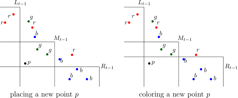
Figure 2: First and second part of the Proof of Theorem 3

We place a new point $p$ south-west of the points in $M_{t-1}$ but south-east from the points of $L_{t-1}$ and north-west from the points of $R_{t-1}$ (see left of Figure 2). This way $p$ is a potential member of all three wedges but only threatens $M_{t-1}$. For any coloring of $p$, we have to pick $L_{t}$, $M_{t}$, and $R_{t}$ such that ${\ell_{t}+1\choose 2}+m_{t}+{r_{t}+1\choose 2}>{\ell_{t-1}+1\choose 2}+m_{t-1}+{r_{t-1}+1\choose 2}$.

If $p$ is given the color of $M_{t-1}$, then let $L_{t}=L_{t-1}$, $M_{t}=M_{t-1}\cup\{p\}$, and $R_{t}=R_{t-1}$, the sum increases by one. Otherwise $p$ is colored with the color of, say, $L_{t-1}$. In this case let $L_{t}=L_{t-1}\cup\{p\}$, $M_{t}=\emptyset$, and $R_{t}=R_{t-1}$. Now

$${\ell_{t}+1\choose 2}+m_{t}+{r_{t}+1\choose 2} ={\ell_{t-1}+2\choose 2}+0+{r_{t}+1\choose 2}$$

$$={\ell_{t-1}+1\choose 2}+\ell_{t-1}+1+{r_{t-1}+1\choose 2}$$

$$\geq{\ell_{t-1}+1\choose 2}+m_{t-1}+1+{r_{t-1}+1\choose 2}.$$

To prove the second statement, we must assign colors online to at most $k^{2}-1$ points to avoid a monochromatic wedge of size $k$. If at time $t$ the new point $p$ is north-east from some earlier point $q$ then we color it to a different color from $q$, this way we do not introduce new monochromatic wedges (but may destroy some). Otherwise, using Proposition 4, when the new point, $p$, arrives, there are two colors that bordering mamos can have. Consider the largest size of these of each color and denote them by $L_{t-1}$ and $R_{t-1}$, and their sizes by $\ell_{t-1}$ and $r_{t-1}$ such that $\ell_{t-1}\leq r_{t-1}$, and let their colors be red and blue. Denote by $m_{t-1}$ the size of the largest mamo $M_{t-1}$ threatened by $p$ having the third color, green. See right of Figure 2. If $\ell_{t-1}\leq m_{t-1}$, then color $p$ red, otherwise color it green. That is, we always color $p$ to the color of a smallest mamo among the three differently colored mamos $L_{t-1},M_{t-1},R_{t-1}$ of which $p$ is a potential member.

We claim that if $a_{t}\leq b_{t}$ are the sizes of the largest pair of mamos with different colors at the end of the step at time $t$, then at least ${a_{t}\choose 2}+{b_{t}\choose 2}$ points have been destroyed by the end of the step at time $t$. To prove this, first see that at one step we add and color only one point thus at most one of $a_{t}$ and $b_{t}$ can increase and only by at most $1$. Further, ${a_{t}\choose 2}+{b_{t}\choose 2}$ can be greater than ${a_{t-1}\choose 2}+{b_{t-1}\choose 2}$ only if all three of $m_{t-1}$, $\ell_{t-1}$, and $r_{t-1}$ are at least $a_{t-1}$, and at least two of them is equal to $a_{t-1}$. In this case $\{a_{t},b_{t}\}=\{a_{t-1}+1,b_{t-1}\}$ (as an unordered pair of integers) and we color the new point $p$ red and destroy at least $a_{t-1}={a_{t-1}+1\choose 2}+{b_{t-1}\choose 2}-\left({a_{t-1}\choose 2}+{b_{t-1}\choose 2}\right)$ green points, proving the claim.

Suppose the first time we obtain a mamo of size $k$ is at the end of step $t$, then we must have $a_{t-1}=b_{t-1}=k-1$, thus we destroyed by the end of step at time $t-1$ at least $2{k-1\choose 2}$ points. Further, we must have $\ell_{t-1}=r_{t-1}=m_{t-1}=k-1$, thus the three differently colored mamos $L_{t-1},M_{t-1},R_{t-1}$ contain $3(k-1)$ non-destroyed points. Together with the $1$ point we add at step $t$, in total we have at least $2{k-1\choose 2}+3(k-1)+1=k^{2}$ points. ∎

For $c\geq 4$ we can give an exponential (in $ck$) lower bound for the number of points we can color.

Theorem 5.

For $c\geq 4$ we can color online with $c$ colors any set of at most $1.22074^{c(k-2)+1}$ points such that throughout the process there is no monochromatic wedge of size $k$. Moreover, if $c$ is large enough, then we can even color online any set of at most $1.46557^{c(k-2)+1}$ points without creating a monochromatic wedge of size $k$. For large $c$, we can color online any set of at most $1.46557^{c}$ points without creating any monochromatic wedges of size $2$.

Before proving the theorem we introduce some notations.

Definition 10.

Let $\mathcal{A}$ be an online coloring algorithm of points in $\mathbb{R}^{2}$. Before step $t$, let $p_{1},p_{2}\ldots,p_{t-1}$ be the $t-1$ points the algorithm has colored so far. In step $t$ the point $p_{t}$ appears and is colored. Define the weights of the points after step $t$, $w_{t}(p_{i})$, $i\leq t$ as

$$w_{t}(p_{i})=\begin{cases}&0,\textrm{ if $p_{i}$ is destroyed by $p_{t}$ in step $t$,}\\ &1+\sum_{p_{j}\textrm{ is destroyed by $p_{t}$ in step }t}w_{t-1}(p_{j}),\textrm{ if }i=t,\\ &w_{t-1}(p_{i})\textrm{ otherwise.}\end{cases}$$ (1)

The weight of a wedge is the sum of the weights of the points in the wedge.

Given an online coloring algorithm $\mathcal{A}$, let $w_{\mathcal{A}}(i,j)$ be the minimal weight of a monochromatic wedge of size $i$ and color $\geq j$ OR size $>i$ and any color over all online point sets colored using algorithm $\mathcal{A}$. If $\mathcal{A}$ is such that there is never such a wedge, then define $w_{\mathcal{A}}(i,j)=\infty$.

Note that after any step $t$ a point that was destroyed at any earlier time has zero weight and that the sum of all the weights after any time $t$ is always equal to the number of arrived points $t$. Note that $w_{\mathcal{A}}(i,1)$ is a lower bound on the minimal number of points in an online point set which contains a monochromatic wedge of size $i$ when colored by $\mathcal{A}$.

Proof of Theorem 5.

First we describe the algorithm how to color a new point. If the new point $p$ is north-east from an earlier point, it is given a different color from one such point. In this case no new monochromatic wedge, and in particular, no new mamo is created. Using Proposition 4, for any new point $p$, there are at most two colors (the border colors) such that any mamos that $p$ borders, are of one of these colors. Every other mamo containing $p$ is threatened. Choose from the non-border colors the color which first minimizes the size of the largest mamo containing $p$ and secondly minimizes the color (as a number from 1 to $c$). Thus our preference is first to have a size $1$ wedge of color $1$, then a size $1$ wedge of color $2$, $\ldots$, size $1$ wedge of color $c$, size $2$ wedge of color $1$, $\ldots$ etc. (with border colors excluded). Figure 1 is an illustration of the algorithm for a 5-coloring.

We now show that this coloring algorithm $\mathcal{A}$ can indeed color the requisite number of points without creating a wedge of size $k$ or more. We will give a lower bound on $w_{\mathcal{A}}(i,j)$ as $w_{\mathcal{A}}(k,1)$ lower bounds the number of points required to make a monochromatic wedge of size $k$. To simplify notation, define $b_{c(i-1)+j}=w_{\mathcal{A}}(i,j)$ for $1\leq j\leq c$ and $b_{n}=0$ for $n\leq 0$. It follows from the definition that $b_{i}\leq b_{j}$ if $i\leq j$. Our goal is to give a good lower bound on $w_{\mathcal{A}}(k,1)=b_{c(k-1)+1}$.

For a mamo of size $i$ and color $j$, order its points in the order as they appeared $p_{1},\dots p_{i}$. Consider the time when the $h^{\text{th}}$ point, $p_{h}$ is added as a new point. Notice that when $p_{h}$ arrives as a new point and we color it, all points of many, previously monochromatic, possibly intersecting wedges will be destroyed. More precisely, from our preferences we have that all points of at least $c-3$ mamos of different colors that are “almost as big” as the one we create by adding $p$ are destroyed. These sizes are at least $h-1$ (and can be more, as when we add $p$ we might create a bigger mamo than $h$) and can be best expressed with the below formula using $b_{n}$. Denote $r=c(h-1)+j$. From the above, using that $b_{n}$ is a monotone increasing sequence, we can show that after adding $p_{h}$, its weight is at least $1+b_{r-3}+b_{r-4}+\ldots+b_{r-c+1}$. Note that $b_{r-1}$ and $b_{r-2}$ are missing from this sum; this is because we had to choose the best available color that is not one of the (at most) two colors of a bordering mamo. This leaves $c-2$ options, of which the mamo whose weight is smallest has weight at least $b_{r-c}$, the next has weight at least $b_{r-c+1}$ and so on, the last has weight at least $b_{r-3}$. Therefore, after choosing the best color, we get that at this step $p_{h}$ destroys at least $b_{r-3}+b_{r-4}+\ldots+b_{r-c+1}$ points, that is

$$w(p_{h})\geq b_{r-3}+b_{r-4}+\ldots+b_{r-c+1}.$$

Therefore, by lower bounding the sum of the weights of the points in a mamo of size $i$ and color $j$, we lower bound $b_{c(i-1)+j}$ and get

$$b_{c(i-1)+j}\geq\sum_{h=1,\dots,i}w(p_{h})\geq\sum_{r=j,c+j,\ldots,c(i-1)+j}1+b_{r-3}+b_{r-4}+\ldots+b_{r-c+1}.$$

To get a lower bound for $b_{r}$, we introduce $a_{r}$ with a non-homogeneous linear recursion $a_{r}=1+a_{r-3}+a_{r-4}+\ldots+a_{r-c}$ starting with $a_{r}=0$ for $r\leq 0$. Notice that for $r\leq c$ we even have $a_{r}=1+a_{r-3}+a_{r-4}+\ldots+a_{r-c+1}$ as $a_{r-c}=0$ in this case. We claim that we have $a_{r}\leq b_{r}$: for $r\leq 0$ this follows from the definition and for $r>0$ we can use induction with the above formula to get

$$b_{c(i-1)+j}\geq\sum_{r=j,c+j,\ldots,c(i-1)+j}1+b_{r-3}+b_{r-4}+\ldots+b_{r-c+1}\geq$$

$$\sum_{r=j,c+j,\ldots,c(i-1)+j}1+a_{r-3}+a_{r-4}+\ldots+a_{r-c+1}=\sum_{r=j,c+j,\ldots,c(i-1)+j}a_{r}-a_{r-c}=a_{c(i-1)+j}.$$

We can reduce the above recursion for $a_{r}$ to a homogeneous linear recursion in several standard ways: by using $a_{r+1}-a_{r}=a_{r-2}-a_{r-c}$; or if $c\geq 4$, by defining $a_{r}^{\prime}=a_{r}+1/(c-3)$; or simply omitting the additive term as it anyway does not affect the order of magnitude. Using either of the above, we can conclude that the magnitude of $a_{r}$, and thus of $b_{r}$, is at least $q^{r}$ where $q$ is the real, root of the equation

$$q^{c}-q^{c-3}-q^{c-4}\ldots-1=0,$$ (2)

which is unique if $c\geq 4$. In order to get an explicit lower bound, notice that $a_{r}\geq 1\geq q^{r-c}$ if $1\leq r\leq c$, and so from the recursion using (2) we also have $a_{r}\geq q^{r-c}$ for all $r$. Among $c\geq 4$, this root is the smallest for $c=4$, in which case we look for the root of $q^{4}-q-1=0$, and a simple numerical calculation shows that this number is larger than $1.22074$. Therefore we have $b_{c(k-1)+1}\geq 1.22074^{c(k-1)+1-c}$, just what was needed. In fact, for $c=4$, the sequence we get is $a_{r}=1+a_{r-3}+a_{r-4}$. Using standard methods, from the recursion we could determine the exact asymptotics of $a_{r}$ for any $c$. As $c$ tends to infinity, the sequence $b_{r}$ is getting closer and closer to the Narayana’s cows sequence $N_{r}=N_{r-1}+N_{r-3}$ [9], and $q$ tends (from below) to the real root of $q^{3}-q^{2}-1=0$, which is bigger than $1.46557$. Therefore, $a_{r}\geq 1.46557^{r}$, if $c$ is large enough. From this we obtain that $a_{c(k-1)+1}\geq 1.46557^{c(k-2)+1}$ if $c$ is large.

To obtain bounds for $k=2$, we should be more careful with the first few terms of the sequence as our initial estimate $a_{r}\geq 1\geq q^{r-c}$ for $1\leq r\leq c$ is not strong enough. The values for small $c$ can be calculated manually, while for larger values we can use the exact value for $N_{r}$, the $r^{\text{th}}$ term of the Narayana’s cows sequence (by Benoit Cloitre [9]) to conclude that $a_{r}>0.6\cdot 1.465571^{r-1}-0.5$. From this we obtain that $b_{c+1}\geq 1.46557^{c}$ if $c$ is large. ∎

In conclusion, if there are $c\geq 4$ colors, the smallest number of points that could force a monochromatic wedge of size $k$ is exponential in $ck$. These bounds can be used to estimate the size of the largest monochromatic wedge when coloring $N$ points with $c$ colors to be $\Theta(\log N/c)$ in the worst case. Similarly for fixed $k\geq 1$, to avoid a monochromatic wedge of size $k$ when coloring $N$ points, $\Theta(\log N/k)$ colors are necessary and sufficient.

Corollary 6.

There is an algorithm to color online $N$ points in the plane using $\Theta(\log N/k)$ colors such that all monochromatic wedges have size strictly less than $k$.

Recall that Lemma 1 stated that $N=2^{n}-1$ points can always force a size $n+1$ color-vector. Theorem 5 implies a lower bound close to this upper bound. Indeed, fix, e.g., $c=4$ and $k=\lceil n/4\rceil$. If the number of points is at most $N=O(1.22074^{n})=O(1.22074^{ck})$, then by Theorem 5 there is an online coloring such that at any time there is no monochromatic wedge of size $k$, thus the size of the color-vector is always at most $4(k-1)<n$.

Observe that the coloring algorithm in the proof of Theorem 5 was oblivious to $k$, thus in fact it implies the following stronger statement.

Corollary 7.

For fixed $c\geq 4$ we can color a countable set of points such that for any $k$, and any $n<1.22074^{c(k-2)+1}$, the first $n$ points of the set are $k$-properly $c$-colored.

This gives an algorithm when $c$ is fixed. Suppose now that $k$ is fixed and we want to use as few colors as possible without knowing in advance how many points will come, i.e., for fixed $k$ we want to minimize $c$ without knowing $N$. To solve this, we alter our previous algorithm. (Note that similarly it is possible to adjust the algorithm for the cases when for an unknown $N$ we want to minimize $\min(c,k)$, or $ck$, and the answer is still logarithmic in $N$.) All this comes with the price of loosing a bit on the base of the exponent. The following theorem implies that for $k=2$ (and thus also for any $k\geq 2$) we can color online any set of $N=O(1.0905^{ck})$ points and if $k$ is big enough, then we can color any set of $N=O(1.1892^{ck})$ points without a monochromatic wedge of size $k$.

Theorem 8.

For fixed $k\geq 1$ we can color a countable set of points such that for any $c$, and any $n<2^{(k-1)\lceil(c-3)/4\rceil+1}-1$, the first $n$ points of the set are $k$-properly $c$-colored.

Proof.

We need to define a coloring algorithm and prove that it uses many colors only if there are many points. Both the coloring and the proof are similar to those in Theorem 5, we only need to change our preferences when coloring. Because of this the analysis of the performance of the algorithm also differs slightly. We fix a $c$ and an $N<2^{(k-1)\lceil(c-3)/4\rceil+1}-1$ for which we will prove the claim of the theorem (the coloring we define will not depend on $c$ or $N$, but only on $k$). Denote the colors by the numbers $\{1,2,\ldots,c,\ldots\}$.

We again avoid the colors of the mamos that border the new point $p$. Denote by $c_{p}$ the color to be assigned to $p$ (as an integer.) Our primary preference now is that we want to keep $\lfloor(c_{p}-1)/4\rfloor$ small. That is, we use one of the four colors $c_{p}$ that minimizes $\lfloor(c_{p}-1)/4\rfloor$ under the condition that using one of these colors we can avoid a monochromatic wedge of size $k$. Once we have these four colors, our secondary preference is that we choose the color from these four colors that minimizes the size of the largest mamo containing $p$. This means that our order of preference is first to have size $1$ wedge of color $1$, $2$, $3$, or $4$, then a size $2$ wedge of color $1$–$4$, $\ldots$, a size $k-1$ wedge of color $1$–$4$, then a size $1$ wedge of color $5$–$8$, $\ldots$ etc. These rules determine our algorithm, except for the choice when more than one of the four colors is possible according to our secondary preference, in which case the chosen color can be arbitrary.

Again let $\mathcal{A}$ be this algorithm and recall that $w_{\mathcal{A}}(i,j)$ refers to the minimal weight of a monochromatic wedge of size $i$ and color $\geq j$ or size $>i$ and any color in an online point set colored using algorithm $\mathcal{A}$. To simplify notations let $b(i,j)=w_{\mathcal{A}}(i,4j)$. Note that by the definition of $\mathcal{A}$, it makes no difference whether we consider $4j-3$, $4j-2$, $4j-1$, or $4j$, we get the same values, that is $w_{\mathcal{A}}(i,j)=b(i,\lceil j/4\rceil)$. Because of this, when it makes no difference, we simply write $4j$ for the color.

We only need to prove that $b(i,j)\geq 2^{(k-1)(j-1)+i}-1$ as this means that if the algorithm uses the color $c+1$, then we had at least $w_{\mathcal{A}}(1,c+1)=b(1,\lceil(c+1)/4\rceil)\geq 2^{(k-1)\lceil(c-3)/4\rceil+1}-1>N$ points, a contradiction. We prove by induction, $b(1,1)=1$. If we introduce a wedge of size $i>1$, we have to destroy all points of at least one mamo of size $i-1$ that had a different color from the same $4$-set, and merged an old mamo of size $i-1$ that had the same color to the new mamo.

Similarly to the proof of Theorem 5, for a mamo of size $i$ and color $4j$, order its points in the order as they appeared $p_{1},\dots p_{i}$ and consider the time when the $h^{\text{th}}$ point, $p_{h}$ is added as a new point. From the above argument, we get $w(p_{h})\geq 1+b(h-1,j)\geq 2^{(k-1)(j-1)+h-1}$ by induction.

Therefore, by lower bounding the sum of the weights of the points in a mamo of size $i$ and color $4j$, we get

$$b_{i,j}\geq\sum_{h=1}^{i}w(p_{h})\geq\sum_{h=1}^{i}2^{(k-1)(j-1)+h-1}=2^{(k-1)(j-1)+i}-1.$$

Finally, we have to check what happens if $i=1$, i.e., if we color a point $p$ with a color $4j$ that has not yet been used. In this case we have to destroy all points of at least two mamos of size $k-1$ having a color from $4j-7$, $4j-6$, $4j-5$, or $4j-4$. Thus $w(p)\geq 1+2b(k-1,j-1)\geq 1+2\cdot(2^{(k-1)(j-2)+k-1}-1)=2^{(k-1)(j-1)+1}-1$. This means that any point of a wedge of color $4j$ has at least this much weight, therefore $b(1,j)\geq 2^{(k-1)(j-1)+1}-1$. ∎

Proposition 9.

The online coloring algorithms guaranteed by the second part of Theorem 3, Theorem 5 and Theorem 8 run in $O(n\log n)$ time to color the first $n$ points (even if we have a countable number of points and $n$ is not known in advance).

The proof of this proposition is omitted as it follows easily from the analysis of the algorithms.

2.2 Online coloring intervals

This section deals with the following interval coloring problem. Given a finite family of intervals on the real line, we want to color them online with $c$ colors such that throughout the process if a point is covered by at least $k$ intervals, then not all of these intervals have the same color.

Proposition 10.

The (online, quasi-online, semi-online) interval coloring problem is equivalent to a restricted case of the problem of $k$-properly (online, quasi-online, semi-online) coloring points with respect to wedges, where we consider only wedges whose apex is on the diagonal line (defined by $y=-x$).

Proof.

Associate to every point $p$ of the diagonal the wedge with apex $p$ and associate with every interval $I=((x_{1},-x_{1}),(x_{2},-x_{2}))$ of the diagonal line the point $(x_{1},-x_{2})$. It is easy to see that $p\in I$ if and only if the point associated to $I$ is contained in the wedge associated to $p$. ∎

Corollary 11.

Any upper bound on the number of colors necessary to (online, quasi-online, semi-online) color wedges in the plane is also an upper bound for the number of colors necessary to (online, quasi-online, semi-online) color intervals in $\mathbb{R}$.

Also the lower bounds of Theorem 2 and of Theorem 3 follow for intervals easily by either repeating the proofs for intervals or by the following observation.

Observation 2.

The proofs of Theorem 2 and of the first part of Theorem 3 can be easily modified such that all the relevant wedges have their apex on the diagonal line.

In particular, we have the following.

Corollary 12.

There is an algorithm to color online $N$ intervals in $\mathbb{R}$ using $\Theta(\log N/k)$ colors such that for every point $x$, contained in at least $k$ intervals, there exist two intervals of different colors containing $x$.

As we have seen, positive results for intervals follow directly from the corresponding results for wedges. Thus all the statements we proved hold for online coloring wedges, also hold for intervals, however, it seems unlikely that the exact bounds are the same. Thus, we would be happy to see (small) examples where there is a distinction. As the next section shows, there is a difference between the exact bounds for quasi-online coloring wedges and intervals.

3 Quasi-online coloring intervals

In this section we consider proper quasi-online coloring an ordered collection of intervals $\{I_{t}\}_{t=1}^{n}$, i.e., proper quasi-online coloring of the dual hypergraph defined by these intervals.

Theorem 13.

Any finite ordered family of intervals on the line can be quasi-online $3$-properly $2$-colored, i.e., colored quasi-online with red and blue such that at any time, for any point contained in at least $3$ intervals, at least one of these intervals is red and another one is blue.

We exploit an idea used in [7]; instead of coloring online the intervals, we online build a labelled acyclic graph (i.e., a forest) with the following properties. At any time $t$, each vertex of the current graph corresponds to an interval on the line, such that for every original interval (i.e., an interval in $\{I_{i}\}_{i=1}^{t}$) there is a corresponding vertex. There might be other vertices in the graph corresponding to auxiliary intervals. In notation, we usually identify a vertex with the corresponding interval, without causing confusion. The final coloring of the intervals is then generated from this graph. In particular, to define a $2$-coloring, we assign each edge in the forest one of two labels, “different” or “same.” For an arbitrary coloring of exactly one vertex in each component (tree) of the graph, there is a unique extension to a coloring of the whole graph compatible with the labelling, i.e., such that each edge labelled “same” is incident to vertices of the same color and each edge labelled “different” is incident to vertices of different colors. We say that a property is forced by the labelling if every compatible coloring has this property. At the end we prove that the forest we built forces the original intervals to be $3$-properly $2$-colored at any time. In [7] all the edges were labelled “different,” so it was actually a simpler variant of our current scheme. As we will see, this idea can also be generalized to more than two colors.

We denote the color of an interval $I$ by $\phi(I)$, the left endvertex of $I$ by $\ell(I)$ and the right endvertex of $I$ by $r(I)$. These vertices are real numbers, and so they can be compared. We can suppose that they are all different, as slightly perturbing them can only make the coloring problem more difficult.

Proof of Theorem 13.

Let $\{I_{t}\}_{t=1}^{n}$ be the given ordered family which has to be quasi-online $3$-properly $2$-colored. We first build the forest and then show that any coloring compatible with this forest is a quasi-online $3$-proper $2$-coloring of the original intervals, as required. As we build the forest we also maintain a family of intervals (corresponding to a subset of the vertices of the forest), called the active intervals. The family of active intervals will change during the process. An interval corresponding to a vertex is not necessarily one of the original intervals, $\{I_{t}\}_{t=1}^{n}$, it might be an auxiliary interval created during the process. At any time $t$ the vertices of the actual forest correspond to the first $t$ original intervals and the auxiliary intervals created up to time $t$. After coloring the forest of the original and auxiliary intervals, we get the desired coloring. We maintain that the following properties hold any time, i.e., for any $t$ after adding interval $I_{t}$ and running step $t$ of the forest-building algorithm (defined later) the following properties hold.

1. Every point of the line is covered by at most two active intervals.

2. No active interval contains another active interval.

3. For any point on the line (at least) one of the following holds.

   • The point is contained in the same number of active intervals as original intervals, and additionally the labelling forces these original intervals and these active intervals to have the same set of colors.

   • The labelling forces that the point is contained in original intervals of different colors.

4. The graph is a forest and each tree in the forest contains exactly one vertex that corresponds to an active interval.

During the forest-building process for an arbitrary point property 3(a) will hold until some moment and then property 3(b) will hold from that moment on. Note that if for some point property 3(b) holds, then it will remain so later, as adding vertices and edges to the graph cannot ruin property 3(b). By property 1, this will guarantee that points in at least $3$ original intervals are contained in both colors. Property 4 ensures that a coloring of the active intervals determines a unique coloring of all the intervals, such that this coloring is compatible with the labelling of the forest. Property 2 is a technical condition.

Now we define the forest-building algorithm. For the first step we simply make the first interval active; our forest will consist of a single vertex corresponding to this interval. In general, at the beginning of step $t$, we have a list of active intervals, ${\cal J}_{t-1}$. Now we add the $t^{\text{th}}$ interval, $I_{t}$, to the forest. See Figure 3 for an example. If $I_{t}$ is covered by at least one active interval, then we choose one, $J\in{\cal J}_{t-1}$ and connect $I_{t}$ to $J$ with an edge labelled “different.” If there is no active interval containing $I_{t}$, we add $I_{t}$ to the family of active intervals. Now if there are active intervals contained in $I_{t}$, then we deactivate all of them (remove from the family of active intervals) and connect each of them to $I_{t}$ in the graph with an edge labelled “different.” This way properties 2 and 4 remain true. For a point $p$ if property 3(a) did hold before adding $I_{t}$ then if it is contained in a just deactivated interval, then at this moment of our algorithm property 3(b) will hold for $p$, otherwise property 3(a) remains true (as the possible change in the set of active intervals containing $p$ is the addition of $I_{t}$, which is an original interval as well).

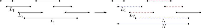
Figure 3: A case in the proof of Theorem 13. Active intervals are represented by solid lines, deactivated intervals by dashed lines.

The last thing we do in step $t$ of our forest-building algorithm is to ensure property 1, i.e., that no point is contained in three active intervals. If there exist such points, they must be contained within $I_{t}$ (as before adding $I_{t}$ by the first property there were no such points). Using the first property, let $L_{1}$ and $L_{2}$ be the (at most) two active intervals covering $\ell(I_{t})$ such that $\ell(L_{1})<\ell(L_{2})$ (if both of them exist). Similarly, let $R_{1}$ and $R_{2}$ be the (at most) two active intervals covering $r(I_{t})$ such that $\ell(R_{1})<\ell(R_{2})$ (if both of them exist). No $L_{i}$ and $R_{j}$ can coincide, as such an interval would cover $I_{t}$. No other active interval can intersect $I_{t}$, as it would necessarily be completely contained in $I_{t}$, but all such intervals are already deactivated. Depending on how many of these four intervals exists, we proceed slightly differently.

First, suppose that there is no $L_{2}$ and $R_{2}$, only $L_{1}$ and $R_{1}$. $L_{1}$ and $R_{1}$ have to intersect, otherwise there is no point covered $3$-fold. This implies that $L_{1}\cup R_{2}$ cover $I_{t}$. We deactivate all three of them and add a new interval $N=L_{1}\cup I_{t}\cup R_{1}$ to the graph and make $N$ active. In the graph, connect $L_{1}$ and $R_{1}$ to $N$ with edges labelled “same” and $I_{t}$ to $N$ with edge labelled “different.”

Next, suppose that all of $L_{1}$, $L_{2}$, $R_{1}$ and $R_{2}$ exist. Deactivate $L_{1}$, $L_{2},I_{t},R_{1}$ and $R_{2}$, and activate a new interval $N=L_{1}\cup I_{t}\cup R_{2}$. In the graph, connect $L_{1},I_{t}$ and $R_{2}$ to $N$ with edges labelled “same.” Connect $L_{2}$ and $R_{1}$ to $N$ with edges labelled “different.”

Otherwise, without loss of generality, suppose that $L_{1}$, $L_{2}$ exists and $R_{2}$ does not exist ($R_{1}$ may or may not exist). Deactivate $L_{1}$, $L_{2}$ and $I_{t}$, and connect them to the new active interval $N=L_{1}\cup I_{t}$ again with the edges of $L_{1}$ and $I_{t}$ labelled “same” and the edge of $L_{2}$ labelled “different.” (Notice that in fact this last case is the same as the first, with $L_{2}$ playing the role of $I_{t}$.)

This way we ensured that property 1 holds and it is easy to check that properties 2 and 4 remain true. Similarly as above, it is easy to check that if for a point property 3(a) did hold then now either property 3(a) or 3(b) holds. Recalling that property 3(b) cannot be ruined we get that property 3 remains true for every point.

By property 4, at the end of the process any coloring of the final family of active intervals extends to a coloring of all the intervals (compatible with the labelling of the graph). We have to prove that for this coloring at any time $t$ any point $p$ contained by at least $3$ of the original intervals is non-monochromatic. At time $t$, by property 1 we have that for such a $p$ property 3(a) cannot hold (as we cannot have $3$ active intervals covering $p$). Thus property 3(b) must hold, which is exactly that $p$ is contained in original intervals of both colors. ∎

Before proceeding with the next proof we define explicitly the structure that the active intervals have during our algorithms (in the previous and in the next proof as well). We call an ordered family of intervals $J_{1},\dots J_{\ell}$ a chain if $\ell(J_{i})<\ell(J_{j})$ and $r(J_{i})<r(J_{j})$ for every $i<j$ and $J_{i}\cap J_{i+1}\neq\emptyset$ for every $i<\ell$ and no point of the real line is contained in three of the intervals. Observe that in a chain any interval $J_{i}$ intersects exactly $J_{i-1}$ and $J_{i+1}$ (if they exist). Two chains are disjoint if the intervals in the first chain is disjoint from the union of the intervals of the second chain.

Theorem 14.

Any finite ordered family of intervals on the line can be quasi-online $2$-properly $3$-colored, i.e., colored quasi-online with $3$ colors such that at any time for any point $p$ contained by at least $2$ of the intervals, the intervals covering $p$ are not all of the same color.

Proof.

We again build an edge-labelled graph $G$, in which vertices correspond to (original and auxiliary) intervals and the label of a directed edge is again one of two labels, “different” or “same.” Again some of the intervals are active. An order on the non-active intervals is appropriate, if putting all active intervals arbitrarily ordered at the end of this order we get an order for which every non-active interval is appropriate: either has at most two forward edges labelled different or at most one forward edge labelled same. Suppose that we could color the active intervals compatibly with $G$, then given an appropriate ordering of the non-active intervals, it is easy to $3$-color these intervals in backwards order to get a $3$-coloring compatible with $G$. During the graph-building algorithm we will maintain such an order of the non-active intervals and also that $G$ induces a union of paths on the active intervals, thus a compatible coloring of $G$ will exist. At the end we prove that such a compatible $3$-coloring of the final graph is necessarily a $2$-proper $3$-coloring at any time.

In the proof we say that we are coloring an interval $I$ differently from (resp. same as) another interval $J$ when we add an edge $IJ$ to $G$ with label different (resp. same). Now we state the required properties.

1. Every point of the line is covered by at most two active intervals.

2. No active interval contains another active interval.

3. For any point on the line (at least) one of the following holds.

   • The point is contained in the same number of active intervals as original intervals, and additionally the labelling forces these original intervals and these active intervals to have the same set of colors.

   • The labelling forces that the point is contained in original intervals of different colors.

4. The order $<_{a}$ of the non-active intervals is appropriate. Also, the family of active intervals induces a union of paths in $G$, more precisely, two active intervals are connected and the connecting edge has label different if and only if they are consecutive in a chain.

Note that the first two properties ensure that, just like in the proof of Theorem 13, at any step the active intervals have a unique partition into disjoint (maximal) chains, thus property 4 is well-defined.

Unlike in the previous proof, now points covered by only two active intervals are also important to us, so property 4 ensures that any two intersecting active intervals receive a different color. In particular, property 3(b) must hold for every point contained in at least $2$ original intervals. Apart from this, the arguments are similar to the ones in the previous proof.

Now we define the graph-building algorithm. During the process, when an interval is deactivated, in $<_{a}$ it is placed after all previously deactivated intervals, that is, at the top of the order $<_{a}$. Also, during the process we never add nor delete an edge incident to any interval that was deactivated earlier, this way all previously deactivated intervals will necessarily remain appropriate. Note that we can and will indeed delete edges sometimes, in which case at the same time we add some edges that force that a compatible coloring with the new graph is necessarily also compatible with the deleted edge, thus the deleted edges are redundant. We do this solely to simplify our presentation.

In the first step we add $I_{1}$ to the (previously empty) graph and activate it. In the inductive step we add $I_{t}$ to the graph and also to the family of active intervals. If $I_{t}$ is covered by an active interval or by the union of two (consecutive) intervals of a chain, then we deactivate $I_{t}$ and color it differently from the interval(s) covering it, i.e., we add at most two edges from $I_{t}$ to active intervals, labelled different. This way $I_{t}$ will be appropriate.

Properties 2 and 4 remain true. For a point $p$ if property 3(a) did hold before adding $I_{t}$, then if it is contained in a just deactivated interval, then at this moment of our algorithm property 3(b) will hold for $p$, otherwise property 3(a) remains true (as the possible change in the set of active intervals containing $p$ is the addition of $I_{t}$, which is an original interval as well).

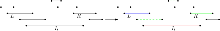
Figure 4: Case i) of Theorem 14

Again, the last thing we do in step $t$ of our graph-building algorithm is to ensure property 1, i.e., that no point is contained in three active intervals. If there is no such point, we are done. Otherwise, such points must be in $I_{t}$. Denote (if exists) by $L$ the active interval with $\ell(L)<\ell(I_{t})$ with the leftmost left end, and by $R$ the active interval with $r(I_{t})<r(R)$ with the rightmost right end that covers a triple covered point. They necessarily intersect $I_{t}$. We distinguish two cases.

Case i) If $I_{t}$ is not covered by the union of the intervals in one chain, then either $L$ or $R$ does not exist, or $L$ and $R$ are not in the same chain. In either case, $I_{t}$ is not covered by $L\cup R$. We deactivate all active intervals covered by $L\cup I_{t}\cup R$, except for $L$, $I_{t}$ and $R$. The rule to color the now deactivated intervals is that they get a color different from $I_{t}$, i.e., for each deactivated interval $J$ we add an edge to $I_{t}$ labelled different. The order in which we deactivate these intervals (and add them to the top of $<_{a}$) is that one-by-one for each chain involved (the chain of $L$, $R$ and the chains in-between) we add first a left-most or right-most interval (in the chain containing $L$ (resp. $R$) it must be the rightmost (resp. leftmost)) and then one-by-one its neighbors. Adding the deactivated intervals in this order to $<_{a}$ ensures that by property 4 such a deactivated interval has at most two forward going edges (one to $I_{t}$ and at most one to one of its neighbors in the path corresponding to this chain).

In the remaining cases $L$ and $R$ exist and are in one chain and $I_{t}$ is covered by the union of the intervals in this chain. Denote by $L_{-}$ and $L_{+}$ (resp. $R_{-}$ and $R_{+}$) the intervals preceding and succeeding $L$ (resp. $R$) in the chain (if they exist).

Case ii) First assume that there are even many intervals in the chain between $L$ and $R$. We insert a new active interval $N$ that we get by taking the union of $L$ and these intervals. We connect $N$ to $L_{-}$ (if it exists) and to $R$ with edges labelled different. Now we deactivate $L$ and color it the same as we color $N$ (we add the edge $NL$ to the graph labelled same and delete the other at most two edges from $L$ to $L_{-}$ and $L_{+}$). We deactivate the intervals between $L$ and $R$ in the chain and color them differently from $I_{t}$. We deactivate them in the left-to-right order, thus they will be appropriate in $<_{a}$ (they have at most two forward edges, one to $I_{t}$ and one to their right neighbor in the chain). We deactivate $I_{t}$ and color differently from the color of $N$ and $R$ (we add the edges $I_{t}N$ and $I_{t}R$ to the graph). We need to check that the deleted edges became redundant. In a compatible coloring $L$ has the same color as $N$, different from $L_{-}$, as required, and also different from $R$, which must get the same color as $L_{+}$ (this is forced by a chain (a path in $G$) of active intervals all colored differently from $I_{t}$ and thus alternating), as required.

Case iii) Next assume that there are odd many intervals between $L$ and $R$. We insert the new active interval $N=L\cup I_{t}\cup R$ and connect it to $L_{-}$ and $R_{+}$ (if they exist) with edges labelled different. Now we again deactivate $L$ and color it the same as we color $N$ (we add the edge $NL$ to the graph labelled same and delete the other at most two edges from $L$ to $L_{-}$ and $L_{+}$). We also deactivate $R$ and color it the same as we color $N$ (we add the edge $NR$ to the graph labelled same and delete the edge from $R$ to $R_{+}$; note that we do not delete the edge $RR_{-}$). We deactivate the intervals in the chain between $L$ and $R$ and color them differently from $I_{t}$. We deactivate them in the left-to-right order, thus they will be appropriate in $<_{a}$ (they have at most two forward edges, one to $I_{t}$ and one to their right neighbor in the chain). We deactivate $I_{t}$ and color differently from the color of $N$ (we add the edge $I_{t}N$ to the graph). We need to check that the deleted edges became redundant. In a compatible coloring $L$ has the same color as $N$, different from $L_{-}$, as required; $R$ has the same color as $N$, different from $R_{+}$, as required; the deactivated intervals from $L+$ to $R$ get the two colors different from the color of $I_{t}$ alternatingly (forced by a chain which is a path in the graph), which ensures that $L$ and $L_{+}$ have different colors, as required.

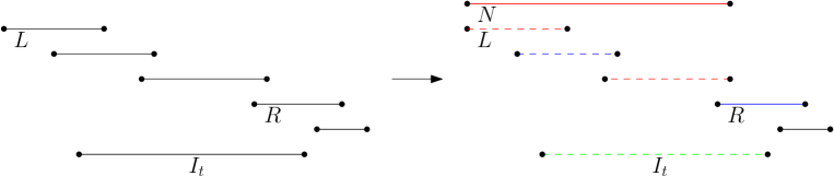
Figure 5: Case ii) of Theorem 14

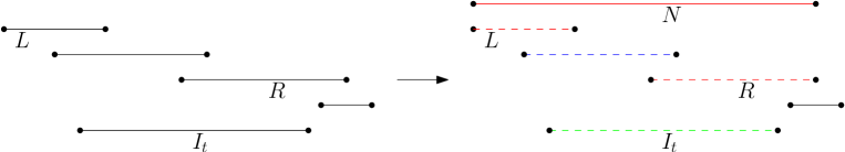
Figure 6: Case iii) of Theorem 14

This way we made sure that property 1 holds and it is easy to check that properties 2 and 4 remain true. It is again easy to check that property 3 also remains true for every point.

By property 4 at the end the active intervals induce a family of paths, which can be easily colored properly (even with $2$ colors). As the ordering $<_{a}$ is appropriate, coloring the non-active intervals in backwards order the coloring extends to a coloring of all the intervals compatible with the labelling of the graph. We have to prove that for this coloring at any time $t$ any point $p$ contained by at least $2$ of the original intervals is non-monochromatic. During the process we just added edges and deleted redundant edges, thus a coloring compatible with the final graph is also compatible with the graph at time $t$. Thus at time $t$, by property 1 we have that such a $p$ is contained in at most two active intervals. If it is contained in exactly two active intervals then by property 4 it is contained in intervals of both colors. Otherwise $p$ is contained in at most one active interval but at least two original intervals, thus property 3(a) cannot hold. Thus property 3(b) must hold, which is exactly that $p$ is contained in original intervals of both colors. ∎

Theorem 15.

Colorings guaranteed by Theorem 13 and Theorem 14 can be found in $O(n\log n)$ time.

Proof.

Instead of a rigorous proof we provide only a sketch, the easy details are left to the reader. In both algorithms we have $n$ intervals, thus $n$ steps. In each step we define a bounded number of new active intervals, thus altogether we have $cn$ original and auxiliary intervals. We always maintain the (well-defined) left-to-right order of the active intervals. We also maintain an order of the (original and auxiliary) intervals such that an interval’s color depends only on the color of one or two intervals’ that are later in this order. This order can be easily maintained as in each step the new interval and the new active intervals come at the end of the order. We also save for each interval the one or two intervals which it depends on. This can be imagined as the intervals represented by vertices on the horizontal line arranged according to this order and an acyclic directed graph on them representing the dependency relations, thus each edge goes backwards and each vertex has in-degree at most two (at most one in the first algorithm, i.e., the graph is a directed forest in that case). In each step we have to update the order of active intervals and the acyclic graph of all the intervals, this can be done in $c\log n$ time plus the time needed for the deletion of intervals from the order. Although the latter can be linear in one step, yet altogether during the whole process it remains $cn$. At the end we just color the vertices one by one from right to left following the rules, which again takes only $cn$ time. Altogether this is $cn\log n$ time. ∎

As we noted earlier, these problems are equivalent to (offline) colorings of bottomless rectangles in the plane. Using this phrasing, Theorem 14 and Theorem 13 were proved already in [5, 4], yet those proofs are quite involved and they only give quadratic time algorithms, so these results are improvements regarding simplicity of proofs and efficiency of the algorithms. The algorithms in [5, 4] proceed with the intervals in backwards order and the intervals are colored immediately, yet in each step many intervals have to be recolored, this might be a reason why a lot of re-colorings are needed there (which we do not need in the above proofs), adding up to quadratic time algorithms (contrasting the near-linear time algorithms above).

References

- [1] P. Cheilaris, B. Keszegh, D. Pálvölgyi, Unique-maximum and conflict-free colorings for hypergraphs and tree graphs, SIAM Journal on Discrete Mathematics, 27(4), 1775–1787, 2013.
- [2] A. Asinowski, J. Cardinal, N. Cohen, S. Collette, T. Hackl, M. Hoffmann, K. Knauer, S. Langerman, M. Lason, P. Micek, G. Rote, T. Ueckerdt, Coloring Hypergraphs Induced by Dynamic Point Sets and Bottomless Rectangles, Algorithms and Data Structures, Lecture Notes in Computer Science 8037 (2013), 73–84.
- [3] J. Cardinal, K. Knauer, P. Micek, T. Ueckerdt, Making Octants Colorful and Related Covering Decomposition Problems, SODA ’14 Proceedings of the Twenty-Fifth Annual ACM-SIAM Symposium on Discrete Algorithms, 1424–1432.
- [4] B. Keszegh: Coloring half-planes and bottomless rectangles, Computational Geometry: Theory and Applications 45(9), Elsevier (2012), 495–507.
- [5] B. Keszegh: Weak conflict free colorings of point sets and simple regions, The 19th Canadian Conference on Computational Geometry (CCCG07), Proceedings, (2007) 97–100.
- [6] B. Keszegh, N. Lemons and D. Pálvölgyi: Online and quasi-online colorings of wedges and intervals, SOFSEM 2013: Theory and Practice of Computer Science, Lecture Notes in Computer Science 7741 (2013), 292–306.
- [7] B. Keszegh, D. Pálvölgyi: Octants are Cover Decomposable, Discrete and Computational Geometry 47(3), Springer (2012) 598–609.
- [8] B. Keszegh, D. Pálvölgyi: Octants are Cover Decomposable into Many Coverings, Computational Geometry Theory and Applications, 47(5) (2014), 585–588.
- [9] Online Encyclopedia of Integer Sequences, https://oeis.org/A000930.
- [10] J. Pach, Decomposition of multiple packing and covering, Diskrete Geometrie, 2. Kolloq. Math. Inst. Univ. Salzburg, 1980, 169–178.
- [11] D. Pálvölgyi, Decomposition of Geometric Set Systems and Graphs, PhD thesis, arXiv:1009.4641 [math.co]
- [12] J. Pach, D. Pálvölgyi, G. Tóth, Survey on Decomposition of Multiple Coverings, in Geometry, Intuitive, Discrete, and Convex (I. Bárány, K. J. Böröczky, G. Fejes Tóth, J. Pach eds.), Bolyai Society Mathematical Studies 24, Springer-Verlag (2014), 219–257.
- [13] Shakhar Smorodinsky, Conflict-Free Coloring and its Applications, in Geometry, Intuitive, Discrete, and Convex (I. Bárány, K. J. Böröczky, G. Fejes Tóth, J. Pach eds.), Bolyai Society Mathematical Studies 24, Springer-Verlag (2014)
- [14] W.T. Trotter, New perspectives on interval orders and interval graphs, in R. A. Bailey (ed.), Surveys in Combinatorics, London Math. Soc. Lecture Note Ser. 241 (1997), 237-286
- [15] G. Tardos: Personal communication