Chapter 13 SOC Systems in Astrophysics

by Markus J. Aschwanden

The universe is full of nonlinear energy dissipation processes, which occur intermittently, triggered by local instabilities, and can be understood in terms of the self-organized criticality (SOC) concept. In Table 2.1 we included a number of cosmic processes with SOC behavior. On the largest scale, galaxy formation may be triggered by gravitational collapses (at least in the top-down scenario), which form concentrations of stars in spiral-like structures due the conservation of the angular momentum. Similarly, stars and planets form randomly by local gravitational collapses of interstellar molecular clouds. Blazars (blazing quasi-stellar objects) are active galactic nuclei that have a special geometry with their relativistic jets pointed towards the Earth, producing erratic bursts of synchrotron radiation in radio and X-rays. Soft gamma repeaters are strongly magnetized neutron stars that produce crust quakes (in analogy to earthquakes) caused by magnetic stresses and star crust fractures. Similarly, pulsars emit giant pulses of radio and hard X-ray bursts during time glitches of their otherwise very periodic pulsar signal. Blackhole objects are believed to emit erratic pulses by magnetic instabilities created in the accretion disk due to rotational shear motion. Cosmic ray particles are the result of a long-lasting series of particle acceleration processes accumulated inside and outside of our galaxy, which is manifested in a powerlaw-like energy spectrum extending over more than 10 orders of magnitude. Solar and stellar flares are produced by magnetic reconnection processes, which are observed as impulsive bursts in many wavelengths. Also phenomena in our solar system exhibit powerlaw-like size distributions, such as Saturn ring particles, asteroids, or lunar craters, which are believed to be generated by collisional fragmentation processes or their consequences (in form of meteroid impacts). The magnetosphere of planets spawns magnetic reconnection processes also, giving rise to substorms and auroras.

While these astrophysical processes have been interpreted in terms of the self-organized criticality concept (for a comprehensive overview see Aschwanden 2011a), quantitative theoretical modeling of astrophysical SOC phenomena is still largely unexplored. In the following Section 13.1 we outline a general theory approach to SOC phenomena, which consists of a universal (physics-free) mathematical/statistical aspect, as well as a physical aspect that is unique to each astrophysical SOC phenomenon or observed wavelength range. In the subsequent Section 13.2 we discuss then the astrophysical observations and compare the observed size distributions with the theoretically predicted ones.

13.1 Theory

A system with nonlinear energy dissipation governed by self-organized criticality (SOC) is usually modeled by means of cellular automaton (CA) simulations (BTW model; Bak et al. 1987, 1988). A theoretical definition of a SOC system thus can be derived from the mathematical rules of a CA algorithm, which includes: (1) A S-dimensional rectangular lattice grid, (2) a place-holder for a physical quantity $z_{i,j,k}$ associated with each cellular node $x_{i,j,k}$, (3) a definition of a critical threshold $z_{crit}$, (4) a random input $\Delta z_{i,j,k}$ in space and time; (5) a mathematical re-distribution rule that is applied when a local physical quantity exceeds the critical threshold value which adjusts the state of the next-neighbor cells, and (6) iterative time steps to update the system state $z_{i,j,k}(t)$ as a function of time $t$. Although this definition is sufficient to set up a numerical simulation that mimics the dynamical behavior of a SOC system, it does not quantify the resulting powerlaw-like size distributions in an explicit way, nor does is include any physical scaling law that is involved in the relationship between statistical SOC parameters and astrophysical observables. A quantitative SOC theory should be generalized in such a way that it encompasses both the mathematical/statistical aspects of a SOC system, as well as the physical scaling laws between observables and statistical SOC parameters. In the following we generalize the fractal-diffusive SOC model (FD-SOC), described in Aschwanden (2012a) and outlined in Section 2.2.2, which includes three essential parts: two universal statistical aspects, i.e., (i) the scale-free probability theorem, (ii) the fractal-diffusive spatio-temporal relationship, and a physical aspect, i.e., (iii) physical scaling laws between geometric SOC parameters and astrophysical observables, which may be different for each observed SOC phenomenon and each observed wavelength in astrophysical data. Some basic examples of physical scaling laws are derived for fragmentation processes, for thermal emission of astrophysical plasmas, and for astrophysical particle acceleration mechanisms.

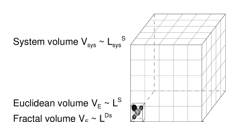
Figure 13.1: The geometric relationships between the Euclidean avalanche volume $V_{E}\propto L^{S}$, the fractal avalanche volume $V\propto L^{D_{s}}$, and the system volume $V_{sys}\propto L_{sys}^{S}$ is visualized in 3D space $(S=3)$, as a function of the avalanche length scale $L$ and system size $L_{sys}$. Note that the probability for an avalanche with size $L$ scales with the ratio of the system volume $V_{sys}$ to the Euclidean avalanche volume $V_{E}$.

13.1.1 The Scale-Free Probability Theorem

Powerlaw-like size distributions are an omnipresent manifestation of SOC phenomena, a property that is also called a “scale-free” parameter distribution, because no preferred scale is singled out by the process. Of course, the scale-free parameter range, over which a size distribution exhibits a powerlaw function, is always limited by instrumental sensitivity or a detection threshold at the lower end, and by the finite length of the time duration over which a SOC system is observed and sampled, at the upper end. Bak et al. (1987, 1988) associated the scale-free behavior with the fundamental property of 1/f-noise that is omnipresent in many physical systems, giving rise to a power spectrum of $P(\nu)\propto\nu^{-1}$.

However, here we give a more elementary explanation for the powerlaw behavior of SOC size distributions, namely in terms of the statistical probability for scale-free avalanche size distributions. A key property of SOC avalanches is that random disturbances can produce both small-scale as well as unpredictable large-scale avalanches of any size, within the limitations of a finite system size $L_{sys}$ at the upper end, and some “atomic” graininess $\Delta L$ at the lower end (i.e., a sand grain in sand avalanches, or the spatial pixel size $\Delta L$ in a computer lattice grid). The statistical probability distribution $N(L)$ for avalanches with size $L$ can be calculated from the statistical probability. If no particular size is preferred in a scale-free process, the number $N(L)$ of possible avalanches in a S-dimensional system with a volume $V_{sys}=L_{sys}^{S}$ is simply the system volume $V_{sys}$ divided by the Euclidean volume $V_{E}=L^{S}$ of a single avalanche with length scale $L$ (Fig. 13.1),

$$N(L)\propto\left({L_{0}\over L}\right)^{S}\propto L^{-S}\ ,$$

In a slowly-driven SOC system, none or only one avalanche happens at one particular time, but the relative probability that an avalanche can happen still scales with the reciprocal volume. This is our first basic assumption of our generalized SOC model, which we call the scale-free probability theorem. This theorem itself predicts a powerlaw function for the basic size distribution of spatial scales, and is distinctly different from the gaussian distribution function that results from binomial probabilities. For 3-dimensional SOC phenomena ($S=3$), thus we expect a size distribution or differential occurrence frequency distribution of $N(L)\propto L^{-3}$, or a cumulative occurrence frequency distribution of $N(>L)\propto L^{-2}$.

We can now derive the expected size distributions for related geometric parameters, such as for the Euclidean avalanche area $A_{E}$ or volume $V_{E}$. If we simply define the Euclidean area $A_{E}$ in terms of the squared length scale, i.e., $A_{E}\propto L^{2}$ or $L\propto A_{E}^{1/2}$, which has the derivative $dL/dA_{E}\propto A_{E}^{-1/2}$, we obtain for the area size distribution $N(A_{E})$, using $N(L)\propto L^{-S}$ (Eq. 13.1),

$$N(A_{E})dA_{E}\propto N[L(A_{E})]\left|{dL\over dA_{E}}\right|dA_{E}\propto A_{E}^{-(1+S)/2}dA_{E}\ ,$$

yielding $N(A_{E})\propto A_{E}^{-2}$ for 3D phenomena ($S=3)$. Similarly we define the Euclidean volume, i.e., $V_{E}\propto L^{3}$ or $L\propto V_{E}^{1/S}$, which has the derivative $dL/dV_{E}\propto V^{1/S-1}$, yielding a volume size distribution $N(V_{E})$,

$$N(V_{E})dV_{E}\propto N[L(V_{E})]\left|{dL\over dV_{E}}\right|dV_{E}\propto V_{E}^{-(2-1/S)}dV_{E}\ ,$$

yielding $N(V_{E})\propto V_{E}^{-5/3}$ for 3D phenomena ($S=3)$.

In the case that avalanche volumes are fractal, such as characterized with a Hausdorff dimension $D_{S}$ in Euclidean space with dimension $S$, the fractal volume $V$ scales as,

$$V\propto L^{D_{S}}\ ,$$

which yields $L\propto V^{1/D_{S}}$ and the derivative $dL/dV\propto V^{(1/D_{S}-1)}$, and thus the size distribution,

$$N(V)dV\propto N[L(V)]\left|{dL\over dV}\right|dV\propto V^{-[1+(S-1)/D_{S}]}\ .$$

The Euclidean limit of non-fractal avalanches would yield for $S=3$ and $D_{S}=S=3$ the same powerlaw index $\alpha_{V}=1+(S-1)/D_{S}=5/3$ as derived for $V_{E}$ in Eq. (13.3). For fractal avalanches, with $D_{S}\approx(1+S)/2=2.0$ for $S=3$, we obtain a slightly steeper powerlaw distribution, $N(V)\propto V^{-2.0}$, than for Euclidean avalanches, i.e., $N(V_{E})\propto V_{E}^{-5/3}$.

A similar effect occurs for fractal avalanche areas $A$. If we assume an fractal structure with Hausdorff dimension $D_{2}$ in 2D space

$$A\propto L^{D_{2}}\ ,$$

which yields $L\propto A^{1/D_{2}}$ and the derivative $dL/dA=A^{1/D_{S}-1}$, and thus a size distribution of

$$N(A)dA\propto N[L(A)]\left|{dL\over dA}\right|dA\propto A^{-[1+(S-1)/D_{2})]}\ .$$

For fractal avalanches, with $D_{2}\approx(1+S)/2=1.5$ for the 2-D fractal dimension, we obtain a powerlaw distribution $N(A)\propto A^{-7/3}$, which is slightly steeper than for Euclidean avalanche areas, i.e., $N(A_{E})\propto A_{E}^{-2.0}$.

In some astrophysical observations, such as in solar and planetary physics, the areas $A$ of SOC phenomena can be measured, while spatially integrated emission (or spatially unresolved emission) in (optically-thin) soft X-ray or extreme-ultraviolet wavelengths is often roughly proportional to the fractal volume $V$ of the emitting source, and thus the size distributions Eqs. (13.5) and (13.7) can be used to test our scale-free probability theorem (Eq. 13.1).

If the scale-free probability theorem (Eq. 13.1) is correct, the derived size distributions for spatial scales $N(L)$, avalanche areas $N(A)$, and avalanche volumes $N(V)$, should be universally valid for SOC phenomena, without any physical scaling laws. They should be equally valid for earthquakes or solar flares, regardless of the physical mechanism that is involved in the nonlinear energy dissipation process of a SOC event. In Section 13.2 we will present some astrophysical measurements of size distributions of such geometric parameters ($L,A$) which can corroborate our assumption of the scale-free probability theorem. Volume parameters ($V$) can usually not directly be measured for astrophysical objects, except by means of stereoscopy or tomography of nearby objects.

13.1.2 The Fractal-Diffusive Spatio-Temporal Relationship

After we have established a framework for the statistics of spatial or geometric parameters of SOC avalanche events, we turn now to temporal parameters, which can be defined by a spatio-temporal relationship. The temporal evolution of SOC avalanches is governed by the complexity of next-neighbor interactions above some threshold value, which has an erratically fluctuating time characteristics according to cellular automaton simulations. However, the mean radius $r(t)$ of an evolving SOC avalanche was found to closely mimic a time dependence of $r(t)\propto t^{1/2}$, which can be associated with a classical random-walk or diffusion process (Aschwanden 2012a). Measurements of the spatial evolution of solar flares, which are considered to be an established SOC phenomenon, revealed a similar evolution, but tend to be sub-diffusive for the analyzed dataset (Aschwanden 2012b). Moreover, the instantaneous avalanche area was found to have a fractal structure, while the time-integrated avalanche area is nearly space-filling and thus can be described with an Euclidean area or volume. These two properties of fractal geometry and diffusive evolution have been combined in the fractal-diffusive SOC avalanche model (FD-SOC) (Aschwanden 2012a). We generalize this concept now also for anomalous diffusion,

$$r(t)\propto\kappa\ t^{\beta/2}\ ,$$

where $\kappa$ is the diffusion coefficient and the diffusive index $\beta$ combines classical diffusion ($\beta=1$), as well as anomlous diffusion ($\beta\neq 1$). Anomalous diffusion processes include both sub-diffusion ($\beta=0...1$), as well as super-diffusion ($\beta=1...2$), also called hyper-diffusion or Lévy flights,

$$r(t)\propto t^{\beta/2}\qquad\left\{\begin{array}[]{ll}\beta<1&\mbox{(sub-diffusion)}\\ \beta=1&\mbox{(classical diffusion)}\\ \beta>1&\mbox{(super-diffusion or L\'{e}vy flights)}\end{array}\right.$$

We show the generic time evolution of a sub-diffusion process with $\beta=1/2$ and a super-diffusion process with $\beta=3/2$ in Fig. 13.2. Anomalous diffusion implies more complex properties of the diffusive medium than a homogeneous structure, which may include an inhomogeneous fluid or fractal properties of the diffusive medium.

The spatio-temporal evolution of an instability generally starts with an exponential growth phase (which we may call the acceleration phase), followed by a saturation or quenching phase (which we may call deceleration phase). In the logistic growth model (Section 2.2.1), the deceleration phase saturates asymptotically at a fixed value, while diffusive models do not converge but slow down progressively with time (Fig. 13.2).

Figure 13.2: Comparison of spatio-temporal evolution models: Logistic growth with parameters $t_{L}=1.0,r_{\infty}=1.0,\tau_{G}=0.1$, sub-diffusion ($\beta=1/2$), classical diffusion ($\beta=1$), Lévy flights or super-diffusion ($\beta=3/2$), and linear expansion ($r\propto t$). All curves intersect at $t=t_{L}$ and have the same speed $v=(dr/dt)$ at the intersection point at time $t=t_{L}$. (Aschwanden 2012b).

The diffusive scaling (Eq. 13.9) implies then also a statistical correlation between spatial $L$ and temporal scales $T$,

$$L\propto T^{\beta/2}\ ,$$

where $T$ is the time duration of a SOC avalanche. From the scale-free probability theorem $N(L)\propto L^{-S}$ (Eq. 13.1) we can then directly compute the expected occurrence frequency distribution $N(T)$ for time durations $T$,

$$N(T)dT\propto N[L(T)]\left|{dL\over dT}\right|dT\propto T^{-[1+(S-1)\beta/2]}\ dT\ .$$

For instance, for 3D SOC phenomena ($S=3$) we expect a powerlaw distribution $N(T)\propto T^{-(1+\beta)}$, which amounts to $N(T)\propto T^{-2.0}$ for classical diffusion, $N(T)\propto T^{-1.5}$ for a sub-diffusion case ($\beta=0.5$), or $N(T)\propto T^{-2.5}$ for a super-diffusion case ($\beta=1.5$). The exponentially growing phase is neglected in this derivation, which implies a slight underestimate of the number of short time scales. Time scales can also directly be measured in most SOC phenomena, and thus provide an immediat test of the fractal-diffusive assumption made here, regardless of the physical process that is involved in the observed signal of SOC avalanches.

13.1.3 Size Distributions of Astrophysical Observables

The previous theory on geometric $(L,A,V)$ and temporal $(T)$ parameters should be universally valid for the statistics of SOC phenomena, and thus constitutes a purely “physics-free” mathematical or statistical property of SOC systems. All other observables of SOC events, however, are related to a physical (nonlinear) energy dissipation process, which needs to be modeled in terms of a correlation or scaling law with respect to the physics-free spatio-temporal SOC parameters. Say, if we observe a physical SOC variable $x$ that has a correlation or powerlaw scaling law of $x\propto L^{\gamma}$ with the geometric SOC parameter $L$, we can infer the expected size distribution $N(x)dx$ by substituting the scaling law.

What is most common in astrophysical observations is the flux $F$ or intensity that is observed in some wavlength range $\lambda$ (with physical units of energy per time), originating from a source with unknown volume $V$. The flux $F(t)$ can exhibit strong fluctuations during an energy dissipation event, but we can characterize the time profile of the event with a peak flux $P$, or with the time-integrated flux, also called fluence (with physical untis of energy), which we may denote with $E$. For optically-thin emission observed in soft X-ray or EUV emission, the emissivity or flux is approximately proportional to the source volume $V$, so it is most useful to quantify a scaling law of the flux $F$ with the 3D volume $V$, which we characterize with a powerlaw index $\gamma$,

$$F\propto V^{\gamma}\ .$$

From the size distribution of the fractal volume $N(V)\propto V^{-[1+(S-1)/D_{S}]}$ (Eq. 13.5) and the scaling law $V\propto F^{1/\gamma}$ (Eq. 13.12) and its derivative $dV/dF\propto F^{1/\gamma-1}$ we can then derive the size distribution $N(F)$ of fluxes $F$,

$$N(F)dF\propto N[V(F)]\left|{dV\over dF}\right|dF\propto F^{-[1+(S-1)/(\gamma D_{S})]}dF\ .$$

which has a typical powerlaw index of $\alpha_{F}\approx 2.0$ (for $S=3$, $D_{S}\approx(1+S)/2\approx 2.0$, and $\gamma\approx 1$). For peak fluxes $P$ we have the same distribution, except for the fractal dimension having its maximum Euclidean value $D_{S}\approx S$, which yields,

$$N(P)dP\propto N[V(P)]\left|{dV\over dP}\right|dP\propto P^{-[1+(S-1)/\gamma S]}dF\ .$$

which has a typical value of $\alpha_{P}\approx 5/3\approx 1.67$. Finally, the total flux or fluence $E=\int F(t)dt\approx FT$, is found to have a size distribution of,

$$N(E)dE\propto N[V(E)]\left|{dV\over dE}\right|dE\propto E^{-[1+(S-1)/(\gamma D_{S}+2/\beta)]}dE\ .$$

which has a typical value of $\alpha_{E}\approx 3/2=1.5$, for $S=3$, $D_{S}\approx(1+S)/2\approx 2.0$, $\gamma\approx 1$, and $\beta\approx 1$.

In summary, if we denote the occurrence frequency distributions $N(x)$ of a parameter $x$ with a powerlaw distribution with power index $\alpha_{x}$,

$$N(x)dx\propto x^{-\alpha_{x}}\ dx\ ,$$

we have the following powerlaw coefficients $\alpha_{x}$ for the parameters $x=L,A,V,T,F,P$, and $E$,

$$\begin{array}[]{ll}\alpha_{L}&=S\\ \alpha_{A}&=1+(S-1)/D_{2}\\ \alpha_{V}&=1+(S-1)/D_{S}\\ \alpha_{T}&=1+(S-1)\beta/2\\ \alpha_{F}&=1+(S-1)/(\gamma D_{S})\\ \alpha_{P}&=1+(S-1)/(\gamma S)\\ \alpha_{E}&=1+(S-1)/(\gamma D_{S}+2/\beta)\\ \end{array}\ .$$

Thus, the various powerlaw indices depend on four fundamental parameters: the Euclidean dimension $S$ of the SOC system, the fractal dimension $D_{S}$ of SOC avalanches, the diffusion index $\beta$ of the SOC avalanche evolution, and the scaling law index $\gamma$ between the observed flux and the SOC avalanche volume. Note, that the powerlaw slopes of the geometric ($L,A,V$) and flux parameters ($F,P$) do not depend on the diffusion index $\beta$, and thus are identical for classical or anomalous diffusion. Only the powerlaw slopes of the length scale, time scale, and peak flux ($L,T,P$) do not depend on the fractal dimension. All flux-related parameters ($F,P,E$) depend on a physical scaling law ($\gamma$), which may be different for every observed wavelength range.

In the following we generally assume 3D SOC phenomena ($S=3$), for which the fractal dimension can be estimated by the mean value between the minimum and maximum dimension where SOC avalanches can propagate coherently via next-neighbor interactions (which limits the minimum fractal dimension to $D_{S,min}\approx 1.0$ and maximum fractal dimension to $D_{max}=S$),

$$D_{S}\approx{D_{S,min}+D_{s,max}\over 2}={(1+S)\over 2}\ ,$$

which yields $D_{3}\approx 2.0$ for $S=3$ and simplifies the powerlaw indices to

$$\begin{array}[]{ll}\alpha_{L}&=2\\ \alpha_{A}&=7/3\\ \alpha_{V}&=2\\ \alpha_{T}&=1+\beta\approx 2\\ \alpha_{F}&=1+1/\gamma\approx 2\\ \alpha_{P}&=1+2/(3\gamma)\approx 5/3\\ \alpha_{E}&=1+1/(\gamma+1/\beta)\approx 3/2\\ \end{array}\ .$$

In astrophysics, the distributions of geometric parameters ($L,A,V$) can only be determined from imaging observations with sufficient spatial resolution (in magnetospheric, heliospheric, and solar physics), while the distributions of all other parameters ($T,F,P$, and $E$) can be measured from any non-imaging observations, such as from point-like stellar objects.

13.1.4 Scaling Laws for Thermal Emission of Astrophysical Plasmas

Solar flares and stellar flares are observed in soft X-ray and extreme-ultraviolet (EUV) wavelengths, where the observed intensity is measured in a particular wavelength range $\lambda$ given by the instrumental filter response function. Soft X-ray and EUV emission is produced by photons via the free-free bremsstrahlung process, free-bound transitions, or radiative recombination. In strong magnetic fields, cyclotron and gyrosynchrotron emission is also produced at radio wavelengths. Soft X-ray and EUV emission occur usually in the optically thin regime, and thus the total emission measure $EM$, which is proportional to the observed intensity in a given wavelength $\lambda$, is proportional to the volume $V$ of the emitting source,

$$F_{\lambda}\propto EM=\int n_{e}^{2}({\bf x})\ dV\propto\ \langle n_{e}^{2}\rangle\ V\ .\\$$

Thus, if the electron density $n_{e}$ in a source would be constant, or the same among different flare events, we would have just the simple relation $F_{\lambda}\propto V^{\gamma}$ (Eq. 13.12) with the scaling law index $\gamma=1$, which is an approximation that is often made. In fact, this is quite a reasonable approximation for measurements with a narrow-band temperature filter, which is sensitive to a particular electron temperature $T_{e}$, and thus probes also a particular range of electron densities $n_{e}$ and plasma pressure $p=2n_{e}k_{B}T_{e}$ that depend on this temperature $T_{e}$, whatever the scaling law between electron temperature $T_{e}$ and electron density $n_{e}$ is.

The proportionality constant between the flux intensity $F_{\lambda}$ and emission measure $EM$ is dependent on the wavelength range $\lambda$, because each wavelength filter is centered around a different temperature range $T_{e}$ that corresponds to the line formation temperature in the observed wavelengths $\lambda$. Physical scaling laws have been derived to quantify the relationship between electron temperature $T_{e}$, electron density $n_{e}$, and the spatial length scale $L_{loop}$ of coronal loops, e.g., by assuming a balance between the heating rate, conductive, and radiative loss rate (i.e., the so-called RTV law; Rosner, Tucker, and Vaiana 1978), being (in cgs-units),

$$T_{e}\approx 1400\ (pL_{loop})^{1/3}\ .$$

which we can express in terms of the electron density $n_{e}$, using the definition of the ideal gas law, $p=2n_{e}k_{B}T_{e}$,

$$n_{e}\approx 1.3\times 10^{9}\left({T_{e}\over 1\ {\rm MK}}\right)^{2}\left({L_{loop}\over 10^{9}\ {\rm cm}}\right)^{-1}\quad[{\rm cm}^{-3}]\ .$$

Thus, if there is no particular correlation between the loop length $L_{loop}$ of the densest flare loops (with the highest emission measure) and the volume $V$ of the active region, the density is only a function of the electron temperature, $n_{e}\propto T_{e}^{2}$. Consequently, if a narrowband temperature filter is used in a soft X-ray or EUV wavelength range, sensitive to a peak temperature $T_{\lambda}$, the corresponding electron density is given in a narrow range also, $n_{e}\propto T_{\lambda}^{2}$, and thus the flux is essentially proportional to the flare volume (according to Eq. 13.20), $F_{\lambda}\propto V^{\gamma}$, with a scaling index of $\gamma\approx 1$. On the other hand, if a different powerlaw index $\gamma\neq 1$ is measured, such an observation would reveal a systematic scaling of some parameters ($T_{e},n_{e},L_{loop}$) of the densest flare loops with the size $L$ of the active region.

Another important quantity we want to calculate is the size distribution of thermal energies $E_{th}$, for which we expect a scaling law of (using Eq. 13.22),

$$E_{th}=3n_{e}k_{B}T_{e}V\propto T_{e}^{3}V/L_{loop}\ ,$$

where the most dominant value of the electron temperature $T_{e}$ is given by the peak of the differential emission measure distribution (DEM). Observationally, it was found that the DEM peak temperature of a flare scales approximately with the size $L$ of a flare, i.e., $T_{e}\propto L$ (Aschwanden 1999), which yields with $V\propto L^{D_{S}}$ (assuming that $L_{loop}$ with the highest emission measure is uncorrelated with the active region size $L$),

$$E_{th}\propto L^{3+D_{S}}\ ,$$

or $E_{th}\propto L^{5}$ for $D_{S}\approx 2.0$ and $S=3$. The size distribution for thermal energies is then expected to be,

$$N(E_{th})dE_{th}=N(L[E_{th}])\left|{dL\over dE_{th}}\right|dE_{th}=E_{th}^{-[1+(S-1)/(3+D_{S})]}dE_{th}$$

which yields $N(E_{th})\propto E_{th}^{-1.4}$ for $S=3$ and $D_{S}\approx 2.0$. However, we have to be aware that this estimate of the thermal energy contained in a flare requires multi-thermal measurements to derive the peak DEM temperature and cannot be obtained from a single narrowband filter measurement. Note that the size distribution of thermal energies with powerlaw index $\alpha_{E_{th}}=1.4$ is very similar to the total energy in photons in any wavelength range, i.e., fluence, $\alpha_{E}=1.5$ (Eq. 13.19).

The foregoing model for the thermal energy requires a scaling law between the flare size $L$ and its statistical temperature $T_{e}$. In practice, however, thermal energies were often estimated in a limited temperature range from the filter ratio of two narrowband filters. Such filter ratio measurements are sensitive to a particular temperature $T_{e}$ and electron density $n_{e}$ (Eq. 13.22), which are then essentially constants in the expression for the thermal energy, and thus the thermal energy is mainly proportional to the volume,

$$E_{th,V}\propto V\ ,$$

so that the size distribution of thermal energies $V$ is identical to the size distribution of volumes $V$, which has a powerlaw slope of $\alpha_{th,V}=\alpha_{V}=1+(S-1)/D_{3}$, yielding values in the range of $\alpha_{th,V}=1.67-2.0$, depending on fractal ($D_{3}\approx(1+S)/2=2$ for $S=3$) or Euclidean ($D_{3}=S=3$) volume measurements.

In some studies, the volume is approximated with a “pill-box” geometry, i.e., the product of the measured flare area $A$ with a constant height $h$ along the line-of-sight, $V=Ah$, which makes the volume proportional to the area, and consequently the thermal energy is mainly proportional to the flare area $A$,

$$E_{th,A}\propto A\ ,$$

leading to a size distribution of $E_{th,A}$ that is identical with that of the area $A$, which has the powerlaw slope $\alpha_{th,A}=\alpha_{A}=1+(S-1)/D_{2}$, yielding values in the range of $\alpha_{th,A}=2.0-2.3$, depending on fractal ($D_{2}\approx(1+S)/2=1.5$) or Euclidean ($D_{2}=2$) area measurements in $S=3$ space. Thus, accurate measurements of these size distributions provide a sensitive tool to diagnose the underlying physical scaling laws and model assumptions.

13.1.5 Scaling Laws for Astrophysical Acceleration Mechanisms

Let us consider some simple examples of particle acceleration processes in astrophysical plasmas, such as solar flares, stellar flares, or cosmic rays. The simplest particle acceleration process is a coherent direct current (DC) electric field, which can be characterized by an acceleration constant $a$ over a system length $L$. Newtonian (non-relativistic) mechanics predicts for an electron with mass $m_{e}$ a velocity $v=at$ after a distance $L=(1/2)at^{2}$, which corresponds to a kinetic energy $E_{L}$ of (where the subscript $L$ refers to the length scale of the accelerator),

$$E_{L}={1\over 2}m_{e}v^{2}=m_{e}aL\ ,$$

which implies a linear energy increase with system length, $E_{L}\propto L$. Thus, the size distribution of energies $E_{L}$ is identical with that of length scales $L$, which we obtain from the scale-free probability theorem $N(L)\propto L^{-S}$ (Eq. 13.1),

$$N(E_{L})dE_{L}=N(L[E_{L}])\left|{dL\over dE_{L}}\right|dE_{L}=E_{L}^{-S}dE_{L}\ ,$$

yielding an energy spectrum $N(E_{L})\approx E_{L}^{-3}$ for a 3D Euclidean volume. This simplest case is given by coherent acceleration thoughout the entire source volume.

Another approach could be made by assuming that the magnetic energy density $dE_{B}/dV=B^{2}/8\pi$ per volume element converted into nonthermal particle energy is uncorrelated with the system size $L$, in which case the total converted magnetic energy just scales with the Euclidean volume $V\propto L^{S}$ of the energy dissipation process, $E_{B}\propto V_{E}\propto L^{S}$. The corresponding size distribution of magnetic energy $E_{B}$ is then expected to scale as,

$$N(E_{B})dE_{B}=N(L[E_{B})\left|{dL\over dE_{B}}\right|dE_{B}=E_{B}^{-(2-1/S)}dE_{B}\ ,$$

which translates into $N(E_{B})\propto E_{B}^{-5/3}$ for a 3D Euclidean volume (S=3). Interestingly, this value is also identical with the size distribution of the peak flux $P$. Alternative scaling laws using the Alfvénic crossing time through the flare volume have also been considered (e.g, Shibata and Yokoyama 1999, 2002; Nishizuka et al. 2008).

Thus, the two acceleration models yield powerlaw size distributions in the range of $\alpha_{E_{B}}=1.67$ to $\alpha_{E_{L}}=3.0$. The measurement of size distributions of nonthermal energies thus can yield valuable diagnostics about the physical nature of the underlying particle acceleration process.

A summary of all theoretically derived powerlaw indices expected in astrophysical systems is compiled in Table 1.

Table 13.1: Summary of powerlaw indices predicted in astrophysical systems, as a function of the dimensionality $S$, the fractal dimension $D_{S}$, the diffusion power index $\beta$, and the energy-volume scaling index $\gamma$.

Parameter	Powerlaw index	Powerlaw index for
	(general expression)	$S=3$, $D_{3}=2$, $D_{2}=3/2$
		$\beta=1$, $\gamma=1$
Length scale $L$	$\alpha_{L}=S$	$\alpha_{L}=3$
Area $A$	$\alpha_{A}=1+(S-1)/D_{2}$	$\alpha_{A}=7/3$
Volume $V$	$\alpha_{V}=1+(S-1)/D_{3}$	$\alpha_{V}=2$
Time duration $T$	$\alpha_{T}=1+\beta$	$\alpha_{T}=2$
Flux $F$	$\alpha_{F}=1+1/\gamma$	$\alpha_{F}=2$
Peak flux $P$	$\alpha_{P}=1+2/(3\gamma)$	$\alpha_{P}=5/3$
Fluence $E$	$\alpha_{E}=1+1/(\gamma+1/\beta)$	$\alpha_{E}=3/2$
Emission measure $EM_{\lambda}$	$\alpha_{EM_{\lambda}}=\alpha_{V}$	$\alpha_{EM_{\lambda}}=2$
Thermal energy $E_{th}$	$\alpha_{E_{th}}=1+(S-1)/(3+D_{S})$	$\alpha_{E_{th}}=7/5$
Thermal energy $E_{th,A}$	$\alpha_{E_{th,A}}=\alpha_{A}$	$\alpha_{E_{th}}=7/3$
Thermal energy $E_{th,V}$	$\alpha_{E_{th,V}}=\alpha_{V}$	$\alpha_{E_{th}}=2$
Linear energy $E_{L}$	$\alpha_{E_{L}}=S$	$\alpha_{E_{L}}=3$
Magnetic energy $E_{B}$	$\alpha_{E_{B}}=(2-1/S)$	$\alpha_{E_{B}}=5/3$

13.2 Observations

We discuss now a number of astrophysical observations with regard to their observed size distributions, which we compare with the foregoing theoretical predictions. A more detailed review of these measurements is given in Aschwanden (2011; chapters 7 and 8).

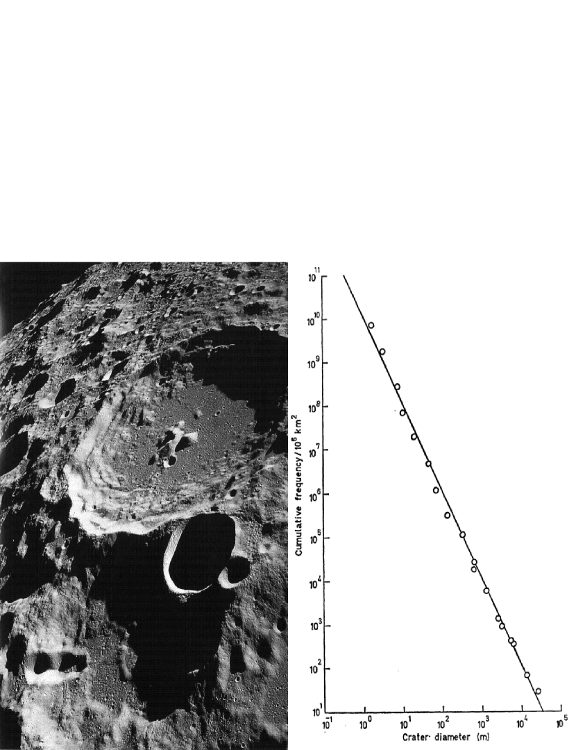
Figure 13.3: Left: The lunar crater Daedalus, about 93 km in diameter, was photographed by the crew of Apollo 11 as they orbited the Moon in 1969 (NASA photo AS11-44-6611). Right: Cumulative frequency distribution of crater diameters measured from Ranger 8 in the lunar Mare Tranquillitatis (Cross 1966).

13.2.1 Lunar Craters

The size of lunar craters was measured from pictures recorded with the lunar orbiters Ranger 7, 8, 9 by Cross (1966). A size distribution of 1,600 lunar craters, sampled in the Mare Tranquillitatis using data from Ranger 8, within a range of 0.56 to 69,000 m, is shown in Fig. 13.3, exhibiting a powerlaw distribution ranging over 5 orders of magnitude with a slope of $\beta\approx 2.0$ for the cumulative occurrence frequency distribution, which translates into a powerlaw slope of $\alpha\approx\beta+1\approx 3.0$ for the differential occurrence frequency distribution,

$$N(L)\propto L^{-3}\ .$$

This corresponds exactly to our prediction of the scale-free probability theorem for avalanche events in 3D-space ($S=3$). A similar powerlaw index of $\alpha_{L}=2.75$ was also found for the size distribution of meteorites and space debris from man-made rockets and satellites (Fig. 3.11 in Sornette 2004).

How can we interpret this result? The justification of our scale-free probability theorem is the fact that the relative probability of partitioning a system into smaller parts scales reciprocally with the volume (Fig. 13.1). The leading theory of lunar crater formation is that their origin was caused by impacts of meteorites, and thus the size distribution reflects that of the impacting meteors and meteorites, which probably were produced by numerous random collisions, similar to the origin of planets, asteroids, and planetesimals. Both the Moon and the Earth were subjected to intense bombardment of solar system bodies between 4.6 and 4.0 billion years ago, which was the final stage of the sweep-up of debris left over from the formation of the solar system.

An alternative explanation of lunar or terrestrial craters is a volcanic origin. If we attribute volcanoes with nonlinear energy dissipation avalanches in a slowly-driven system of stressing planet crust motions and build-up of subtectonic lava pressure, volcanic eruptions can also be understood as SOC phenomena.

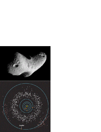
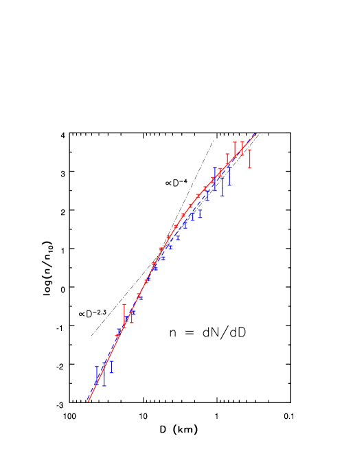
Figure 13.4: Left top: A picture of the near-Earth asteroid Eros with a size of 30 km, pictured by a space probe. Left bottom: The main asteroid belt located between the Jupiter and Mars orbit. The subgroup of Trojan asteroids are leading and trailing along the Jupiter orbit. (Courtesy of NASA/Johns Hopkins University Applied Physics Laboratory). Right: Differential size distribution of asteroids observed in the Sloan Digital Sky Survey collaboration (Ivezic et al. 2001).

13.2.2 Asteroid Belt

The asteroid size distribution has been studied in the Palomar Leiden Survey (Van Houten et al. 1970) and Spacewatch Surveys (Jedicke and Metcalfe 1998), where a power law of $N^{cum}(>L)\propto L^{-1.8}$ was found for the cumulative size distribution of larger asteroids ($L>5$ km), which corresponds to a differential powerlaw slope of $\alpha_{L}\approx 2.8$. In a Sloan Digital Sky Survey collaboration (Fig. 13.4, right), a broken powerlaw was found with $N(L)\propto L^{-2.3}$ for large asteroids (5-50 km) and $N(L)\propto L^{-4}$ for smaller asteroids (0.5-5 km) (Ivezic et al. 2001). In the Subaru Main-Belt Asteroid Survey, a cumulative size distribution $N^{cum}(>L)\propto L^{-1.29\pm 0.02}$ was found for small asteroids with $L\approx 0.6-1.0$ km (Yoshida et al. 2003; Yoshida and Nakamura 2007), which corresponds to a differential powerlaw slope of $\alpha_{L}\approx 2.3$. Thus, the observed range $\alpha_{L}\approx 2.3-4.0$ of the powerlaw slopes of length scales $L$ is centered around the theoretically expected value of $\alpha_{L}=3.0$, predicted by our scale-free probability theorem.

The origin of asteroids is thought to be a left-over distribution of planetesimals during the formation of planets, which were either too small to form bigger planets by self-gravitation, or orbited in an unstable region of the solar system where Mars and Jupiter constantly cause gravitational disturbances that prevented the formation of another planet. Thus, the final distribution of the asteroid belt is likely to be influenced by both the primordial distribution of the solar system as well as by recent collisions and further fragmentation of planetesimals. The collisional fragmentation process can be considered as a mechanical instability that occurs in a multi-body gravitational field. The collisional process is self-organizing in the sense that the N-body celestial mechanics keeps the structure of the asteroid belt more or less stable, despite of the combined effects of self-gravity, gravitational disturbances, collisions, depletions, and captures of incoming new bodies. The quasi-stability of the asteroid belt warrants the critical threshold in form of a finite collision probability maintained by the proximity of the co-orbiting asteroid bodies.

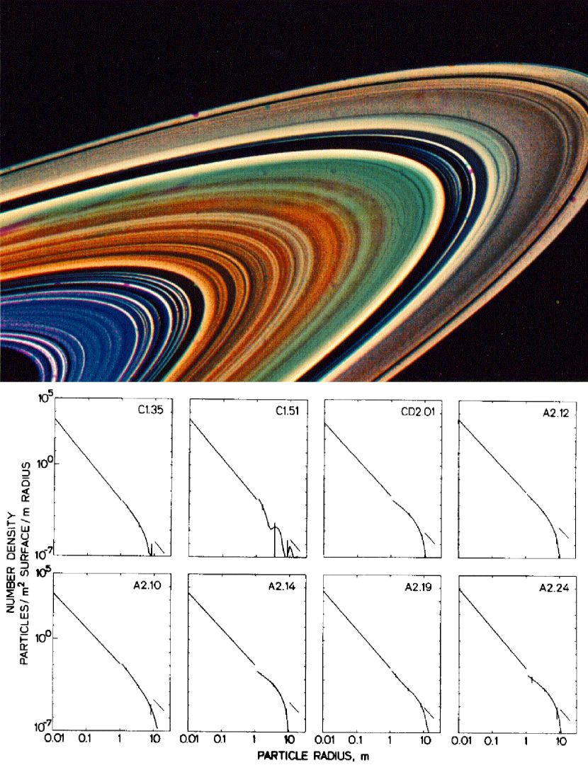
Figure 13.5: Top: Saturn’s rings A, B, C, and the Cassini division, photographed by the Cassini spacecraft (credit: NASA, JPL, Space Science Institute). Bottom: Measurements of the particle size distribution functions for 8 ring regions with Voyager I radio occultation measurements (Ring C: C1.35, C1.51; Cassini division: CD2.01; Ring A: A2.12, A2.10, A2.14, A2.19, A2.24). The slopes of the fitted powerlaw functions in these 8 regions are: $\alpha_{L}=$ 3.11, 3.05, 2.79, 2.74, 2.70, 2.75, 2.93, 3.03. The range of particle sizes is $L=0.01-10$ m (Zebker et al. 1985).

13.2.3 Saturn Ring

The distribution of particle sizes in Saturn’s ring was determined with radio occultation observations using data from the Voyager 1 spacecraft and a scattering model, which exhibited a powerlaw distribution of $N(r)\propto r^{-3}$ (Fig. 13.5) in the range of 1 mm $<$ r $<$ 20 m (Zebker et al. 1985; French and Nicholson 2000). The size distribution revealed slightly different powerlaw slopes in each ring zone, e.g., $\alpha_{L}=2.74-3.03$ for ring A, $\alpha_{L}=2.79$ for the Cassini division, or $\alpha_{L}=3.05-3.22$ for ring C (Zebker et al. 1985). These results, again, are consistent with a fragmentation process that obeys the scale-free probability theorem, similar to the distribution of sizes of asteroids and lunar craters, and predicts a size distribution of $N(L)\propto L^{-3}$. The conclusion that Saturn’s ring particles are formed from the (collisional) breakup of larger particles, rather than from original condensation as small particles, was already raised earlier (Greenberg et al. 1977).

The Saturn ring, which consists of particles ranging in size from 1 cm to 10 m, is located at a distance of 7,000-80,000 km above Saturn’s equator, and has a total mass of $3\times 10^{19}$ kg, just about a little less than the moon Mimas. The origin of the ring is believed to come either from leftover material of the formation of Saturn itself, or from the tidal disruptions of a former moon. The celestial mechanics of the Saturn rings is quite complex, revealing numerous gaps in orbits that have a harmonic ratio in their period with one of the 62 (confirmed) moons (with 13 moons having a size larger than 50 km). Similar to the asteroid belt, the Saturn ring can be considered as a self-organizing system in the sense that the gravity of Saturn and the gravitational disturbances caused by Saturn’s moons keep the ring quasi-stable, which provides a critical threshold rate for collisional encounters due to the proximity of the co-orbiting ring particles.

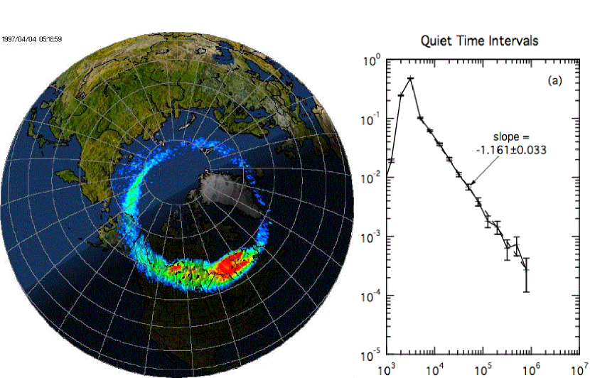
Figure 13.6: Left: Global image of the auroral oval observed by the Ultraviolet Imager (UVI) onboard the NASA satellite “Polar” on April 4, 1997 at 0519 UT, projected onto an Earth map (credit: NASA, Polar/UVI Team, George Parks). Right: Occurrence rate frequency distributions of auroral blobs as a function of the area (in units of square kilometers) during substorm-quiet time intervals, recorded with Polar UVI during Jan 1-31, 1997 (Lui et al. 2000).

13.2.4 Magnetospheric Substorms and Auroras

The size distribution of auroral areas have been measured with the UV Imager of the Polar spacecraft, which exhibits a powerlaw-like distribution with a slope of $\alpha_{A}=1.21\pm 0.08$ during active substorm time intervals, and $\alpha_{A}=1.16\pm 0.03$ during quiescent time intervals (Fig. 13.6; Lui et al. 2000). The corresponding energy flux or power output $P$ of auroral regions was derived to have a powerlaw slope of $\alpha_{P}=1.05\pm 0.08$ during active substorm time intervals, and $\alpha_{P}=1.00\pm 0.02$ during quiescent time intervals (Lui et al. 2000). These powerlaw slopes are significantly flatter than predicted by our FD-SOC model, i.e., $\alpha_{A}=2.33$ and $\alpha_{P}=1.67$ for 3D phenomena ($S=3,D_{2}\approx 1.5$). Although Lui et al. (2000) interpret auroras as a SOC phenomenon, the observed powerlaw slopes are far out of the range observed and predicted for other SOC phenomena. Thus, either the sampled distributions are incomplete, they underestimate the areas systematically for smaller events, or SOC models are not applicable for these events.

Plasma flows in the magnetotail plasma with speeds $v\geq 400$ km s^-1 were found to have a powerlaw distribution of durations $T$, with $N(T)\propto T^{1.59\pm 0.07}$ (Angelopoulos et al. 1999), which is not too far off our theoretical prediction (with $\alpha_{T}=2.0$), given the relatively small powerlaw range of only $\approx 1.5$ decades. Also the size distributions of the durations of AE index ($\alpha=1.24$; Takalo 1993; Takalo et al. 1999) and AU index ($\alpha=1.3$; Freeman et al. 2000; Chapman and Watkins 2001) were found to be much flatter than predicted by our SOC model.

Electron bursts in the outer radiation belt (at $4-8$ L-shell distances), which may be modulated by fluctuations of the solar wind, were found to have powerlaw distributions with slopes of $\alpha_{P}=1.5-2.1$ and were interpreted as SOC phenomena (Crosby et al. 2005), which have slopes that are quite consistent with our SOC model ($\alpha_{P}=1.67$). The solar wind is thought to be the source of these energetic electrons, although the solar wind velocity frequency distributions were found to exhibit significant deviations from simple powerlaws (Crosby et al. 2005).

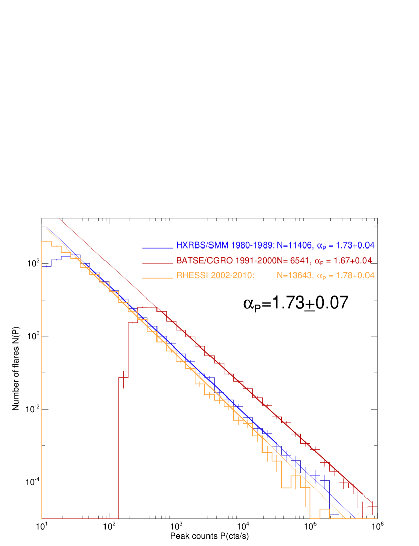
Figure 13.7: Occurrence frequency distributions of hard X-ray peak count rates $P$ [cts s^-1] observed with HXRBS/SMM (1980 – 1989), BATSE (1991 – 2000), and RHESSI (2002 – 2010), with powerlaw fits. An average pre-flare background of $40$ [cts s^-1] was subtracted from the HXRBS count rates. Note that BATSE/CGRO has larger detector areas, and thus records higher count rates (Aschwanden 2011b).

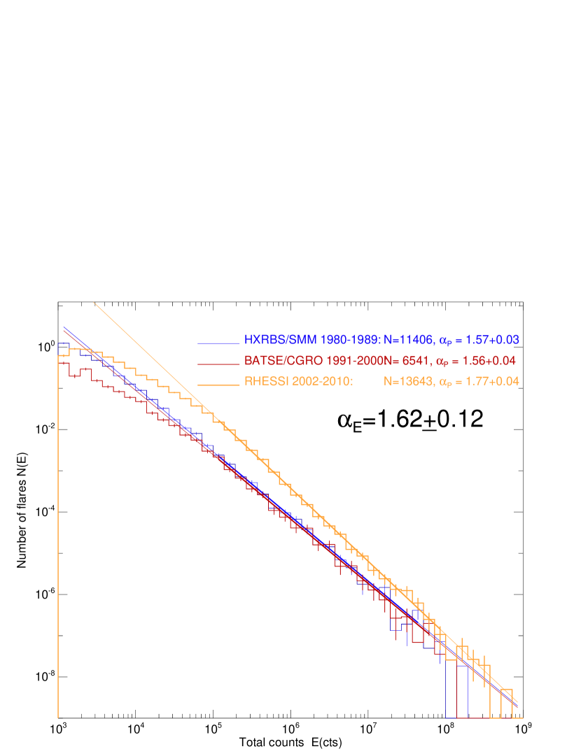
Figure 13.8: Occurrence frequency distributions of hard X-ray total counts or fluence $E$ [cts] observed with HXRBS/SMM (1980 – 1989), BATSE (1991 – 2000), and RHESSI (2002 – 2010), with powerlaw fits. An average pre-flare background of $40$ cts s^-1 multiplied with the flare duration was subtracted in the total counts of HXRBS (Aschwanden 2011b).

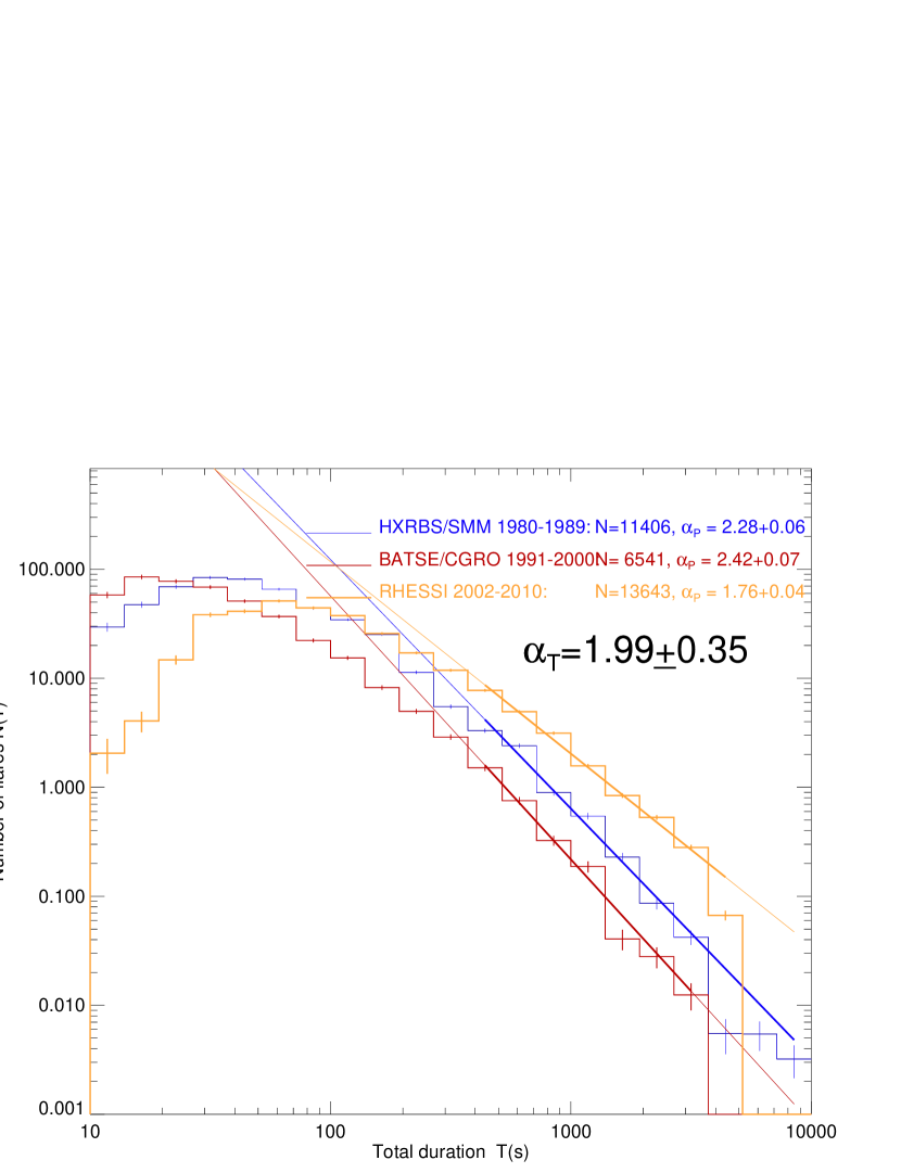
Figure 13.9: Occurrence frequency distributions of hard X-ray flare durations $T$ [s] observed with HXRBS/SMM (1980 – 1989), BATSE (1991 – 2000), and RHESSI (2002 – 2010) with powerlaw fits. The flare durations for RHESSI were estimated from the time difference between the start and peak time, because RHESSI flare durations were determined at a lower energy of 12 keV (compared with 25 keV for HXRBS and BATSE), where thermal emission prolonges the nonthermal flare duration (Aschwanden 2011b).

13.2.5 Solar Flares

Solar flares are the best studied SOC phenomena in astrophysics. The impulsive energy release associated with solar flares, which can be observed in virtually all wavelengths, from gamma-rays, hard X-rays, soft X-rays, EUV, white-light, infrared, to radio wavelengths, has been interpreted as a SOC phenomen from early on (Lu and Hamilton 1991). Large datasets with $n\approx 10^{4}-10^{5}$ events sampled over up to eight orders of magnitude in energy provide the necessary statistics to determine accurate slopes of the observed powerlaw-like size distributions. However, major challenges exist still in the elimination of sampling biases in incomplete event sets, the understanding and modeling of powerlaw slopes in different wavelengths in terms of the underlying physical scaling laws, and the automated determination of geometric parameters for large event datasets. A detailed account of observational results sorted into different wavelength regimes is given in Aschwanden (2012a; chapters 7 and 8). We summarize the results of powerlaw slopes observed in size distributions of various SOC parameters in Table 13.2, selecting mostly representative examples with large datasets from different instruments and wavelength regimes.

Size distributions of peak fluxes $P$ (Fig. 13.7), time-integrated fluxes or fluences $E$ (Fig. 13.8), and flare durations $T$ (Fig. 13.9), have been measured for energies $>25$ keV in hard X-ray wavelengths with instruments on the spacecraft ISEE-3, SMM, CGRO, and RHESSI, in soft X-ray wavelengths with Yohkoh and GOES, and in EUV with SOHO/EIT, TRACE, and AIA/SDO. Most of the observed powerlaw slopes were measured close to the theoretical predictions, i.e., $\alpha_{T}=2.0$, $\alpha_{P}=1.67$, and $\alpha_{E}=1.5$ (Table 13.2), which is consistent with a dimensionality of $S=3$, a mean fractal dimension of $D_{S}\approx(1+S)/2=2.0$, an energy-volume scaling index of $\gamma\approx 1$, and a diffusion power index of $\beta\approx 1$ (Eq. 13.17 and 13.19).

The measurements in soft X-rays and hard X-rays are all made in broadband energy and wavelength ranges, and thus are least biased regarding a complete sampling of all energy and temperature ranges. The probably most controversial measurements have been made for the smallest flares, also called nanoflares, which have typical temperatures of $T\approx 1-2$ MK and originate in small loops that barely stick out of the transition region. Since EUV measurements with SOHO/EIT, TRACE, and AIA/SDO are all made with narrowband temperature filters, the inferred thermal energies essentially scale with the flare area (Eq. 13.27) or volume (Eq 13.26), for which we predict powerlaw slopes of $\alpha_{th,A}\approx\alpha_{A}\approx 2.3$ and $\alpha_{th,V}\approx\alpha_{V}\approx 2.0$, which are significantly steeper than what is predicted for thermal energies sampled with broadband instruments, i.e., $\alpha_{th}\approx 1.5$. This sampling bias has resulted into a controversy whether nanoflares dominate coronal heating, because a powerlaw slope steeper than the critical value of 2 indicates that the energy integral diverges for the smallest events, as pointed out early on (Hudson 1991). Synthesizing measurements from narrowband EUV instruments with broadband soft X-ray instruments, as well as taking the fractal geometry of flare structures into account, however, could reconcile the size distribution for nanoflares with that of large flares with a corrected value that is close to the theoretical prediction of $\alpha_{E}\approx 1.5$ (Fig. 13.10; Aschwanden and Parnell 2002).

Problematic are also the measurements of flare durations $T$ for several reasons, such as the limited range of durations over which a powerlaw can be fitted, the ambiguity of separating overlapping long-duration flares, and the solar cycle dependence. While the event overlap problem is not severe during the solar minimum, where a slope close to the theoretically predicted value of $\alpha_{T}=2.0$ is measured, the flare event pile-up bias becomes very severe during the solar maximum, producing powerlaw slopes of up to $\alpha_{T}\lower 1.72218pt\hbox{$\;\buildrel<\over{\scriptstyle\sim}\;$}5$ (Aschwanden and Freeland 2012). Also the powerlaw slope of hard X-ray peak counts $\alpha_{P}$ appears to reveal a solar cycle dependence due to a similar effect (Bai 1993, Biesecker 1994, Aschwanden 2011b).

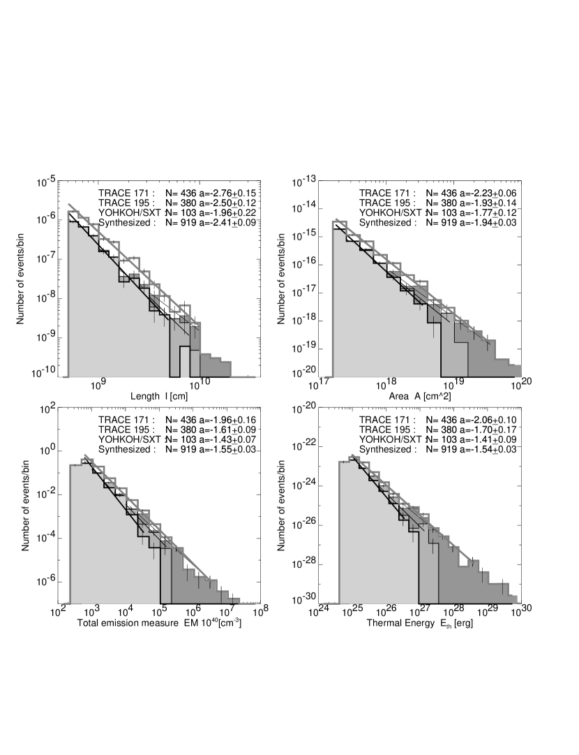
Figure 13.10: Synthesized frequency distributions from all three wavebands (TRACE 171 Å, 195 Å, and Yohkoh/SXT AlMg) (grey histograms), along with the separate distributions from each waveband (in greyscales). Each of the distributions is fitted with a powerlaw, with the slope values and formal fit errors given in each panel. The four panels represent the four parameters of length $L$, area $A$, total emission measure $EM$ (which is proportional to the peak flux $P$), and the thermal energy $E_{th}$ (Aschwanden and Parnell 2002).

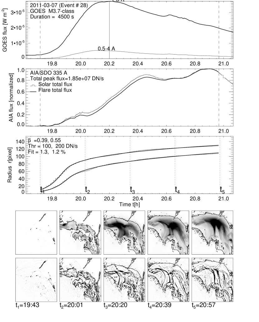
Figure 13.11: A solar flare event is observed on 2011 Mar 7, 19:43-20:58 UT, with AIA/SDO 335 Å, with GOES time profiles (top panel), the total EUV 335 Å flux (second panel), the spatio-temporal evolution of the radius $r(t)=\sqrt{A(t)/\pi}$ of the time-integrated flare area $A(t)$ for two thresholds, $F_{thresh}=100,200$ DN/s (third panel; histogrammed), fitted with the anomalous diffusion model (third panel; solid curve), and 5 snapshots of the baseline-subtracted flux (fourth row) and highpass-filtered flux (bottom row), with the threshold flux $F_{thresh}=100$ DN/s shown as contour (Aschwanden 2012b).

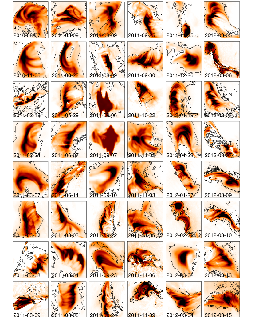
Figure 13.12: A selection of 48 solar GOES M and X-class flares observed with AIA/SDO at a wavelength of 335 Å during 2010-2012. The contour shows the time-integrated flare area and the color-scale represents the intensity at 335 Å. Note the complex spatial patterns that ressemble to the fractal avalanche patterns of cellular automaton simulations.

The least explored size distributions of solar flares are the length scale $L$ and area $A$ size distributions. Relatively small samples of flare areas have been measured for EUV nanoflares (Aschwanden et al. 2000, Aschwanden and Parnell 2002) and for the largest M and X-class flares (Aschwanden 2012b). Since the measurement of these parameters provides a direct test of the scale-free probability theorem (Eq. 13.1), without depending on any other physical parameter or model assumption, priority should be given to such measurements. Existing measurements have large error bars in the powerlaw slope due to the small number of analyzed events, but are largely consistent with the theoretical prediction of $\alpha_{L}=3.0$ and $\alpha_{A}=2.33$, calculated for 3D SOC avalanches ($S=3$) with a 2D (area $S=2$) fractal dimension of $D_{2}\approx(1+S)/2=1.5$.

Besides the scale-free probability theorem, a second pillar of our FD-SOC model is the fractal-diffusive spatio-temporal relationship $L(t)\propto\kappa T^{\beta/2}$ (Eq. 13.8), which has been recently tested for a set of the 155 largest (GOES M and X-class) flare events (Aschwanden 2012b). An example of such a measurement of the spatio-temporal evolution is shown in Fig. 13.11, which exemplifies the spatial complexity of a large cluster of subsequent magnetic reconnection events that form a fractal volume filled with postflare loops. Examples of another 48 large flares (GOES M and X-class) are shown in Fig. 13.12. Interestingly, the statistics of these 155 largest flares revealed a sub-diffusive regime ($\beta=0.53\pm 0.27$), while classical diffusion appears to be an upper limit. The diffusive characteristics measured in solar flares is consistent with the FD-SOC model, as it is was also found to be consistent with cellular automaton SOC simulations (Aschwanden 2012a).

Radio bursts are produced in solar flares most frequently either by gyrosynchrotron emission of relativistic electrons that have been accelerated in magnetic reconnection regions, or by electron beams that escape along magnetic field lines in upward-direction. Both types of radio bursts (microwave bursts and type III bursts) occur as a consequence of a plasma instability, and thus represent a highly nonlinear energy dissipation process that is typical for SOC processes.

Somewhat ouf the predicted range are solar energetic particles, which have rather flat size distributions $N(P)$ of the peak counts, typically in the range of $\alpha_{P}\approx 1.1-1.4$. However, since these are all high-energy particle events ($>10$ MeV protons and $>3$ MeV electrons), we suspect that only the largest flares produce such high energies, and thus the sample is biased towards the largest flare events, which explains the flatter powerlaw slopes as a consequence of missing weaker events.

Figure 13.13: Cumulative frequency distributions of flare energies (total counts) observed for 12 cool (type F to M) stars with EUVE (Audard et al. 2000). The flare events are marked with diamonds, fitted with a powerlaw fit in the lower half (P; thick line), and fitted with a cumulative frequency distribution (C; curved function).

13.2.6 Stellar Flares

Impulsive flaring with rapid increases in the brightness in UV or EUV has been observed for a number of so-called flare stars, such as AD Leo, AB Dor, YZ Cmi, EK Dra, or $\epsilon$ Eri. These types of stars include cool M dwarfs, brown dwarfs, A-type stars, giants, and binaries in the Hertzsprung-Russell diagram. Most of these stars are believed to have hot soft X-ray emitting coronae, similar to our Sun (a G5 star), and thus magnetic reconnection processes are believed to operate in a similar way as on our Sun.

However, what is different, is that the soft X-ray emission is several orders of magnitude stronger than from our Sun, if we put the stars into the same distance, and thus we expect an observational selection bias towards the largest possible flares. Another difference in flare statistics is that the meagre observational time allocation in the order of a few hours per star reveals only very few detectable flare events, in the order of 5-15 events per observed star. A consequence of this small-number statistics is that we cannot determine a powerlaw slope from a log(N)-log(S) histogram, as we do for larger statistics (of at least $10^{2}$ up to $10^{5}$ events in solar flare data sets), but need to resort to rank-order plots, which correspond to the inverse distribution of cumulative occurrence frequency distributions. So, in principle, an inverse rank-order diagram can be plotted as shown in Fig. 13.13, which shows the logarithmic rank versus the flare energy (or total counts) for each star, from which the powerlaw slope can be determined. However, if we deal with cumulative size distributions, we have also to be aware of the drop-off that results at the upper end of the distribution due to the missing part in the powerlaw differential occurrence frequency distribution above the largest event. Thus, while a straight powerlaw function with slope $\alpha$ can be fitted to a differential frequency distribution $N(E)$,

$$N(E)\propto E^{-\alpha}\ ,$$

the following function need to be fitted to the cumulative distribution $N_{cum}(>E)$ (Aschwanden 2011a, section 7),

$$N_{cum}(>E)=n{\int_{E}^{E_{max}}N(E^{\prime})dE^{\prime}\over\int_{E_{min}}^{E_{max}}N(E^{\prime})dE^{\prime}}=n{\int_{E}^{E_{max}}E^{\prime-\alpha}dE^{\prime}\over\int_{E_{min}}^{E_{max}}E^{\prime-\alpha}dE^{\prime}}=n{(E^{1-\alpha}-E_{max}^{1-\alpha})\over(E_{min}^{1-\alpha}-E_{max}^{1-\alpha})}\ .$$

The fit of this function to the cumulative distribution is shown in Fig. 13.13 for a set of 12 flare stars, and the resulting values for the powerlaw slope $\alpha_{E}$ of the inferred differential occurrence frequency distributions (labeled with the letter $C$ in Fig. 13.13). For comparison, we fit also a straight powerlaw with slope $\beta=\alpha-1$ to the lower half of the cumulative distribution, which is less effected by the upper cutoff (labeled with the letter $P$ in Fig. 13.13). In Table 13.2 we summarize the means and standard deviations of the powerlaw slopes of flare energies observed on flare stars (see individual values in Table 7.7 of Aschwanden 2011a), which have been reported based on various other methods used by the authors, $\alpha_{E}=2.17\pm 0.25$. Fitting only the lower half of the distribution functions we find a significantly lower value of $\alpha_{E}=1.85\pm 0.31$, or by fitting Eq. (13.33) we find a similar range of $\alpha_{E}=1.93\pm 0.35$. This subtle difference in the determination of the powerlaw slope is essential, because it discriminates whether the total energy radiated during stellar flares is dominated by the largest flares (if $\alpha_{E}<2.0$) or by nanoflares (if $\alpha_{E}>2.0$; Hudson 1991). At this point it is not clear whether the difference in the powerlaw slopes obtained for stellar versus solar flares is due to a methodical problem of small-number statistics, or due to a sampling bias for super-large stellar flares, by solar standards.

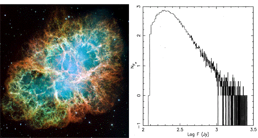
Figure 13.14: Left: Crab nebula, which harbors the pulsar in the center (photographed by Hubble Space Telescope, NASA). Right: Frequency distribution of giant-pulse flux densities measured from the Crab pulsar, observed during 15-27 May 1991 with the Green Bank 43-m telescope at 1330, 800, and 812.5 MHz. The tail can be represented by a powerlaw distribution $N_{F}\propto F^{-\alpha}$ with $\alpha=3.46\pm 0.04$ for fluxes $F>200$ Jy (Lundgren et al. 1995).

13.2.7 Pulsars

Pulsars are fast-spinning neutron stars, which emit strictly periodic signals in radio wavelengths, as well as occasional giant pulses that represent glitches in the otherwise regular pulse amplitude and frequency. The glitches in pulse amplitude and frequency shifts correspond to large positive spin-ups of the neutron star, probably caused by sporadic unpinning of vortices that transfer momentum to the crust. Conservation of the angular momentum produces then an increase of the angular rotation rate. Thus, these giant pulses reveal highly nonlinear energy dissipation processes that can be considered as a SOC phenomenon and we expect a powerlaw function for their size distribution.

Early measurements of the pulse height distribution of the Crab pulsar (NGC 0532 or PSR B0531+21) observed at 146 MHz were indeed found to have a powerlaw slope of $\alpha_{P}\approx\beta+1=3.5$ over a range of 2.25 to 300 times the average pulse size, in a sample of 440 giant pulses (Argyle and Gower 1972). Similar values were measured by Lundgren et al. (1995) in a sample of 30,000 giant pulses, with $\alpha_{P}\approx 3.06-3.36$ (Fig. 13.14, right). While the Crab pulsar is the youngest known pulsar (born in the year 1054), PSR B1937+21 is an older pulsar with a 20 times faster period (1.56 ms) than the Crab pulsar (33 ms). Cognard et al. (1996) measured a powerlaw distribution with a slope of $\alpha_{P}\approx\beta+1=2.8\pm 0.1$ from a sample of 60 giant pulses for this pulsar. Statistics of nine other pulsars revealed powerlaw slopes in a much larger range of $\alpha_{E}=-0.13,...,2.4$ for the size distribution of pulse glitches (Melatos et al. 2008), but those measurements were obtained from much smaller samples of 6-30 giant pulses, and thus represent small-number statistics.

The typical value of $\alpha_{P}\approx 3.0$ found in two pulsars deviates significantly from the prediction ($\alpha_{P}=1.67$) of our FD-SOC model, and thus requires either a different model or more statistics from other pulsar cases. Preliminary values of small samples from other pulsars indicate a wide range ($\alpha_{E}=-0.13,...,2.4$, Melatos et al. 2008) that do not point towards a particular value that can be explained with a single model.

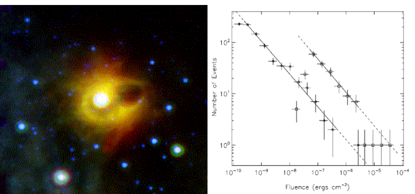
Figure 13.15: Left: The Soft Gamma-Ray Repeater SGR 1900+14 in the constellation of Aquila photographed with the Spitzer Space Telescope in infrared (courtesy: NASA). Right: Differential frequency distributions of the fluences of soft gamma-ray repeater SGR 1900+14 observed with CGRO, RXTE, and ICE (Gogus et al. 1999).

13.2.8 Soft Gamma-Ray Repeaters

Gamma-ray bursts were observed from a variety of astrophysical objects, such as neutron stars or black holes, but usually only one burst has been observed from each object. An exception is a class of objects that show repetitive emission at low-energy gamma-rays ($>25$ keV), which were termed soft gamma-ray repeaters (GRS). Observations with the Compton Gamma Ray Observatory (CGRO) revealed four such SGR sources up to 1999, three in our galaxy and one in the Magellanic Cloud). At least three of these SGR objects were associated with slowly rotating, extremely magnetized neutron stars that are located in supernova remnants (Kouveliotou et al. 1998, 1999). It is believed that these soft gamma-ray bursts occur from neutron star crust fractures driven by the stress of an evolving, ultrastrong magnetic field in the order of $B\lower 1.72218pt\hbox{$\;\buildrel>\over{\scriptstyle\sim}\;$}10^{14}$ G.

Occurrence frequency distributions of the fluence of soft gamma-ray repeaters were obtained from four SGR sources: a database of 837 gamma-ray bursts from SGR 1900+14 during the 1998-1999 active phase showed a powerlaw slope of $\alpha_{E}=1.66$ over 4 orders of magnitude (Fig. 13.15; Gogus et al. 1999); and a combined database from SGR 1806-20, using 290 events detected with the Rossi X-Ray Timing Explorer, 111 events detected with CGRO/BATSE, and 134 events detected with the International Cometary Explorer (ICE), showing power laws with slopes of $\alpha_{E}$=1.43, 1.76, and 1.67 (Gogus et al. 2000). These measurements agree remarkably well with the frequency distributions predicted by the FD-SOC model ($\alpha_{E}=1.50$) as well as with those observed during solar flares, which were also observed at the same hard X-ray energies of $>25$ keV. However, the physical energy dissipation mechanism may be quite different in a solar-like star and a highly magnetized neutron star, given the huge difference in magnetic field strengths ($B\approx 10^{2}$ G for solar flares versus $B\approx 10^{14}$ G in a magnetar), although magnetic reconnection processes could be involved in both cases. Nevertheless, soft gamma-ray repeaters have been interpreted as a SOC system (Gogus et al. 1999), in terms of a neutron star crustquake model (Thompson and Duncan 1996), in analogy to the SOC interpretation of earthquakes.

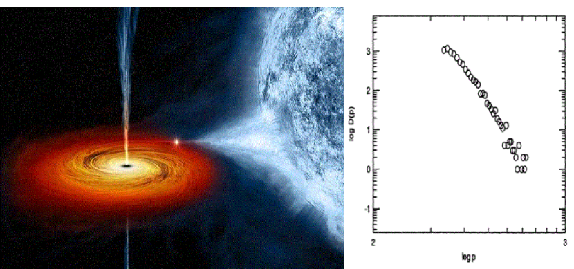
Figure 13.16: Left: This artist concept of Cygnus X-1 shows the black hole drawing material from a companion star (right) into a hot, swirling accretion disk that surrounds the (invisible) black hole (Courtesy of Chandra X-Ray Observatory, NASA). Right: Observed frequency distribution of the peak intensities of pulses in the light curve of the black-hole object Cygnus X-1, exhibiting a powerlaw slope of $\alpha_{P}\approx 7.1$ (Negoro et al. 1995; Mineshige and Negoro 1999).

13.2.9 Black Hole Objects

Cygnus X-1, a galactic X-ray source in the constellation Cygnus, is the first X-ray source that has been widely accepted to be a black-hole candidate. The mass of Cygnus X-1 is estimated to be about 14.8 solar masses and it has been inferred that the object with (an event horizon at) a radius of 26 km is far too compact to be a normal star. Cygnus X-1 is a high-mass X-ray binary star system, which draws mass from a blue supergiant variable star (HDE 226868) in an orbit of 0.2 AU around the black hole. The stellar wind of this blue companion star swirls mass onto an accretion disk around the black hole (Fig. 13.16). The X-ray time profile from Cygnus X-1 reveals time variability down to 1 ms, which is attributed to X-ray pulses from matter infalling toward the black hole and the resulting turbulence in the accretion disk.

Observations of the X-ray light curve of Cygnus X-1 with Ginga exhibit a complex power spectrum that entails at least 3 piece-wise powerlaw sections, which have been interpreted as a superposition of multiple 1/f-noise spectra (Takeuchi et al. 1995). The occurrence frequency distribution of peak intensities shows a powerlaw-like function with a steep slope of $\alpha_{P}\approx 7.1$ (Fig. 13.16 right; Negoro et al. 1995; Mineshige and Negoro 1999). All these properties have been modeled with a sophisticated cellular automaton model in the framework of the SOC concept. Infalling mass lumps in the accretion disk are thought to trigger turbulent instabilities in the neighborhood of an infall side, which propagate avalanche-like and produce hard X-rays either by collisional bremsstrahlung or some other magnetically driven instability (e.g., a magnetic reconnection process). The cellular automaton simulations (Takeuchi et al. 1995, Mineshige and Negoro 1999) were able to reproduce steep powerlaw slopes of the peak fluxes in the range of $\alpha_{P}\approx 5.6-11.5$, depending on the effect of enhanced mass transfer by gradual diffusion in addition to the avalanche-like shots, and this way could reproduce the observations.

We note that the observed steep powerlaw slopes of peak fluxes ($\alpha_{P}\approx 7.1$) exceed the predictions of the FD-SOC model ($\alpha_{P}=1.67$) by far. Such a steep slope, $\alpha_{P}=1+2/(3\gamma)\approx 7$, can be produced by an extremely weak dependence of the X-ray flux $F$ on the avalanche volume $V$, i.e., $F\propto V^{\gamma}$ with $\gamma\approx 1/9$, which is different from the flux-volume scaling law of optically-thin soft X-ray or EUV emission ($\gamma\approx 1$) generally observed in astrophysical sources, and thus may indicate a nonthermal emission mechanism. Alternatively, the very steep powerlaw slope of $\alpha_{P}$ could by part of an exponential frequency distribution near the upper cutoff, which could only be proven by sampling peak fluxes with higher sensitivity. Simultaneous modeling of the observed occurrence frequency distributions of time scales, peak fluxes, and power spectra in terms of a SOC model may reveal the underlying physical scaling law of the emission mechanism in black-hole accretion disks.

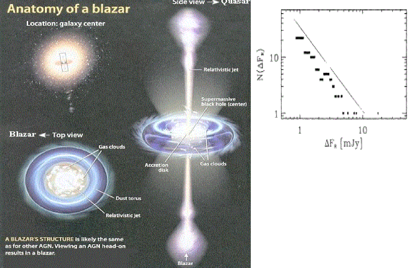
Figure 13.17: Left: The anatomy of a blazar is shown in a top view and side view, having the rotation axis with the relativistic jet oriented toward Earth or orthogonal to the line-of-sight (Courtesy of The Encylopedia of Science). Right: Frequency distribution of peak fluxes of flaring events in blazar GC 0109+224, including fluxes above a 3$\sigma$-threshold, fitted with a powerlaw function $N(P)\propto P^{-1.55}$ (Ciprini et al. 2003).

13.2.10 Blazars

Blazars (blazing quasi-stellar objects) are a special subgroup of quasars. This group includes BL Lacertae objects, high polarization quasars, and optically violent variables. They are believed to be active galactic nuclei whose jets are aligned within $\lower 1.72218pt\hbox{$\;\buildrel<\over{\scriptstyle\sim}\;$}10^{\circ}$ of our line-of-sight (Fig. 13.17 left). Because we are observing “down” the jet direction we observe a large degree of variability and apparent superluminal speeds from the jet-aligned emission. The structure of blazars, like all active galactic nuclie, is thought to be powered by material falling onto the supermassive black hole at the center of the host galaxy, which emits highly intermittent gyrosynchrotron emission (in radio wavelengths), inverse Compton emission (in X-rays and gamma-rays), and free-free bremsstrhalung emission (in soft X-rays), modulated by the variable rate of matter infalling into the accretion disk of the central black hole.

The optical variability of blazar GX 0109+224 was monitored and the light curves were found to exhibit flickering and shot noise, with a power spectrum $P(\nu)\propto\nu^{-p}$ with power index of $p=1.57-2.05$ (Ciprini et al. 2003). The occurrence frequency distribution of peak fluxes of flare events was found to have a powerlaw slope of $\alpha_{p}=1.55$ (Fig. 13.17, right; Ciprini et al. 2003), which is close to the prediction of the FD-SOC model ($\alpha_{p}=1.67$). Thus, the highly-variable blazar emission was interpreted in terms of SOC models. The fact that the peak size distribution of radio emission observed in the blazar agrees with the prediction of the FD-SOC model is consistent with a near-proportional radio flux-volume scaling, i.e., $F\propto V^{\gamma}$ with $\gamma\approx 1$, which is generally the case for gyro-synchrotron emission. This is different from the flux scaling of emission observed from the black hole Cygnus X-1. Thus, SOC statistics allows us to discriminate between different physical emission mechanisms in black holes and blazars.

,

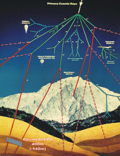
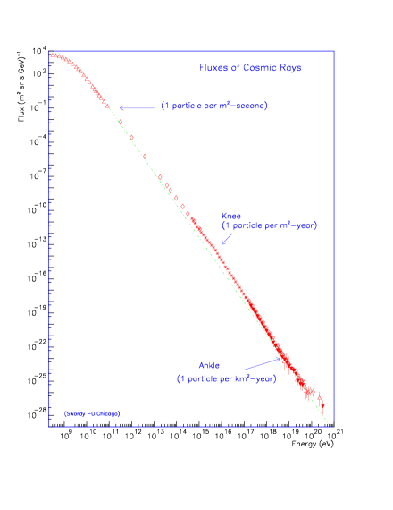
Figure 13.18: Left: The diagram shows the cascade shower of a primary cosmic ray particle, which produces in the Earth’s atmosphere a shower of secondary particles, which can be detected by an unterground detector, such as CosmoALEPH (courtesy of CosmoALEPH Team). Right: Cosmic ray spectrum in the energy range of $E=10^{9}-10^{21}$ eV, covering over 12 orders of magnitude. There is a “knee” in the spectrum around $E\approx 10^{16}$ eV, which separates cosmic rays originating within our galaxy (at lower energies) and those from outside the galaxy (at higher energies). (Credit: Simon Swordy, University of Chicago).

13.2.11 Cosmic Rays

Cosmic rays are high-energy particles that have been accelerated during a long journey through a large part of our universe, inside our Milky way as well as from outside of our galexy. Their boosting to the highest energies of up to $\lower 1.72218pt\hbox{$\;\buildrel<\over{\scriptstyle\sim}\;$}10^{21}$ eV can only occur by multi-step acceleration processes throughout the universe over long time spans. The energy spectrum of cosmic rays, as it can be measured from showers of secondary particles produced in the Earth atmosphere (Fig. 13.18 left), exhibits a powerlaw-like energy spectrum extending from $\approx 10^{9}$ eV (=1 GeV) over 12 orders of magnitude up to $\lower 1.72218pt\hbox{$\;\buildrel<\over{\scriptstyle\sim}\;$}10^{21}$ erg (Fig. 13.18 right). The average slope is $\alpha_{E}\approx 2.7$. However, a more accurate model is a broken powerlaw with a “knee” in the spectrum around $E\approx 10^{16}$ eV. The widely accepted interpretation of this knee is that it separates the origin of cosmic rays from inside and outside of our galaxy. The powerlaw slope above the “knee” steepens to $\alpha_{E}\approx 3.0-3.3$. Interestingly, our FD-SOC model applied to the kinetic energy gain in a coherent direct current (DC) electric field implies a proportionality of $E_{L}\propto L$ (Eq. 13.28) for sub-relativistic energies, and thus predicts an energy distribution of $N(E_{L})\propto E_{L}^{-3}$, similar to the cosmic ray spectrum. Of course, cosmic rays are highly relativistic and are likely to be produced by many $(n)$ acceleration phases. However, even if each acceleration phase is local and has a relatively small length of $l\ll L$, the energy gain of the particle would add up linearly with increasing travel time and travel distance $\sum l$ and could still fulfill the proportionality,

$$E_{L}\propto\sum_{i=1}^{n}E_{l}\propto\sum_{i=1}^{n}l\propto L\ ,$$

and end up with an energy spectrum of $N(E_{L})\propto L^{-3}$.

So, can we understand the acceleration of a cosmic ray as a SOC process? The lattice grid would cover a large fraction of the extragalactic space of our universe, the ensemble of cosmic-ray particles would represent an avalanche that nonlinearly dissipates energy from local acceleration processes (such as by the first-order Fermi acceleration process between intergalactic or interstellar magnetic clouds), which are self-organizing in the sense that accelerating fields (of magnetic clouds) are constantly restored by the galactic and interstellar dynamics.

Our fractal-diffusive spatio-temporal relationship ($r(t)\propto t^{\beta/2}$, Eq. 13.8) further predicts a random-walk through the universe and an age $T$ that scales as $L\propto T^{1/2}$ with the straight travel distance $L$ from the point of origin of the cosmic ray particle. Using the “knee” in the cosmic-ray energy spectrum (at $E_{gal}\approx 10^{16}$ eV) as a calibration for the distance of the Earth to the center of our galaxy ($L_{gal}\approx 50$ light years $\approx 5\times 10^{22}$ cm), we can estimate the straight length scale over which the cosmic ray particle travelled by random walk

$$L_{max}\approx L_{gal}\left({E_{max}\over E_{gal}}\right)\ ,$$

which yields $L_{max}\approx 5\times 10^{27}$ erg, which corresponds to about 10% of the size of our universe $r_{uni}\approx 4\times 10^{28}$. Since the acceleration efficiency is different in galactic and extragalactic space, the diffusion coefficient of the random walk is also different and therefore we expect a different powerlaw slope in the energy spectrum produced in these two regimes.

13.3 Conclusions

In this chapter we generalized the fractal-diffusive self-organized criticality (FD-SOC) model in terms of four fundamental parameters: (i) the Euclidean dimension $S$, (ii) the fractal dimension $D_{S}$ of the spatial SOC avalanche structure, (iii) the diffusion index $\beta$ that includes both sub-diffusion and super-diffusion, and (iv) the energy-volume scaling law with powerlaw index $\gamma$. This model predicts powerlaw functions for the occurrence frequency distributions of the SOC model, and moreover predicts their powerlaw slope as a function of the four fundamental parameters. For a Euclidean dimension of $S=3$, a mean fractal dimension of $D_{S}\approx(1+S)/2=2$, classical diffusion ($\beta=1$), and linear flux-volume scaling ($\gamma=1$), our generalized FD-SOC model predicts then the following powerlaw slopes: $\alpha_{L}=3$ for length scales, $\alpha_{A}=2.333$ for areas, $\alpha_{T}=2$ for durations, $\alpha=1.667$ for peak fluxes, and $\alpha_{E}=1.5$ for fluences or total energies of the SOC avalanches.

Comparing these theoretical predictions with the observed powerlaws of size distributions in astrophysical systems (summarized in Table 13.2) we find acceptable agreement for the cases of lunar craters, asteroid belts, Saturn rings, outer radiation belt electron bursts, solar flares, soft gamma-ray repeaters, and blazars, if we apply the linear flux-volume scaling. Discrepancies are found for magnetospheric substorms, stellar flares, pulsar glitches, black holes, and cosmic rays, which apparently require a nonlinear flux-volume scaling. Pulsar glitches and cosmic rays can indeed be modeled by assuming a linear energy-length scaling, which leads to energy spectra of $N(E)\approx E^{-3}$. Black-hole pulses have very steep size spectra, which indicates a quenching or saturation process that prevents a large variation of pulse amplitudes. Magnetospheric substorms and solar energetic particles have the flattest size distributions, which possibly can be explained by a selection effect with a bias for the largest events. In conclusion, the generalized FD-SOC model can explain a large number of astrophysical observations and can discriminate between different scaling laws of astrophysical observables. We envision that more refined scaling laws between astrophysical observables will be developed that are consistent with the observed size distributions, and this way will provide the ultimate predictive power for SOC models.

Table 13.2: Summary of theoretically predicted and observed powerlaw indices of size distributions in astrophysical systems.

	Length	Area	Duration	Peak flux	Fluence
	$\alpha_{L}$	$\alpha_{A}$, $\alpha_{th,A}$	$\alpha_{T}$	$\alpha_{P}$	$\alpha_{E}$
FD-SOC Theory	3.0	2.33	2.0	1.67	1.50
Lunar craters:
Mare Tranquillitatis ${}^{1})$	3.0
Meteorites and debris ${}^{2})$	2.75
Asteroid belt:
Spacewatch Surveys${}^{3})$	2.8
Sloan Survey${}^{4})$	2.3-4.0
Subaru Survey${}^{5})$	2.3
Saturn ring:
Voyager 1${}^{6})$	2.74-3.11
Magnetosphere:
Active substorms${}^{7})$		$1.21\pm 0.08$		$1.05\pm 0.08$
Quiet substorms${}^{7})$		$1.16\pm 0.03$		$1.00\pm 0.02$
Substorm flow bursts${}^{8})$			$1.59\pm 0.07$
AE index bursts${}^{9})$			1.24
AU index bursts${}^{10})$			1.3
Outer radiation belt${}^{11})$				1.5-2.1
Solar Flares:
ISEE-3, HXR12			1.88-2.73	1.75-1.86	1.51-1.62
HXRBS/SMM, HXR13			$2.17\pm 0.05$	$1.73\pm 0.01$	$1.53\pm 0.02$
BATSE/CGRO, HXR14			2.20-2.42	1.67-1.69	1.56-1.58
RHESSI, HXR15			1.8-2.2	1.58-1.77	1.65-1.77
Yohkoh, SXR16	1.96-2.41	1.77-1.94		1.64-1.89	1.4-1.6
GOES, SXR17			2.0-5.0	1.86-1.98	1.88
SOHO/EIT, EUV18		2.3-2.6	1.4-2.0
TRACE, EUV19	2.50-2.75	2.4-2.6		1.52-2.35	1.41-2.06
AIA/SDO, 335 A, EUV20	1.96		2.17	1.34
Microwave bursts21				1.2-2.5
Type III bursts22				1.26-1.91
Solar energetic particles23				1.10-2.42	1.27-1.32
Stellar Flares:
Flare stars (reported)24					$2.17\pm 0.25$
Flare stars (powerlaw fit)24					$1.85\pm 0.31$
Flare stars (cumulative fit)24					$1.93\pm 0.35$
Astrophysical Objects:
Crab pulsar25				3.06-3.50
PSR B1937+2126				$2.8\pm 0.1$
Soft Gamma-Ray repeaters27					$1.43-1.76$
Cygnus X-1 black hole28				7.1
Blazar GC 0109+22429				1.55
Cosmic rays30					$2.7-3.3$

References to Table 13.2: ${}^{1})$ Cross (1966); ${}^{2})$ Sornette (2004); ${}^{3})$ Jedicke and Metcalfe (1998); ${}^{4})$ Ivezic et al. (2001); ${}^{5})$ Yoshida et al. (2003), Yoshida and Nakamura (2007); ${}^{6})$ Zebker et al. (1985), French and Nicholson (2000); ${}^{7})$ Lui et al. (2000); ${}^{8})$ Angelopoulos et al. (1999); ${}^{9})$ Takalo (1993), Takalo et al. (1999); ${}^{10})$ Freeman et al. (2000); Chapman and Watkins (2001); ${}^{11})$ Crosby et al. (2005) ${}^{12})$ Lu et al. (1993), Lee et al. (1993); ${}^{13})$ Crosby et al. (1993); ${}^{14})$ Aschwanden  (2011a,b); ${}^{15})$ Christe et al. (2008), Lin et al. (2001), Aschwanden  (2011a,b); ${}^{16})$ Shimizu (1995), Aschwanden and Parnell (2002); ${}^{17})$ Lee et al. (1995), Feldman et al. (1997), Veronig et al. (2002a,b), Aschwanden and Freeland (2012); ${}^{18})$ Krucker and Benz (1998), McIntosh and Gurman (2005); ${}^{19})$ Parnell and Jupp (2000), Aschwanden et al. 2000, Benz and Krucker (2002), Aschwanden and Parnell (2002), Georgoulis et al. (2002); ${}^{20})$ Aschwanden (2012b) ${}^{21})$ Akabane (1956), Kundu (1965), Kakinuma et al. (1969), Das et al. (1997), Nita et al. (2002); ${}^{22})$ Fitzenreiter et al. (1976), Aschwanden et al. (1995), Das et al. (1997), Nita et al. (2002); ${}^{23})$ Van Hollebeke et al. (1975), Belovsky and Ochelkov (1979), Cliver et al. (1991), Gabriel and Feynman (1996), Smart and Shea (1997), Mendoza et al. (1997), Miroshnichenko et al. (2001), Gerontidou et al. (2002); ${}^{23})$ Gabriel and Feynman (1996); ${}^{24})$ Robinson et al. (1999), Audard et al. (2000), Kashyap et al. (2002), Güdel et al. (2003), Arzner and Güdel (2004), Arzner et al. (2007), Stelzer et al. (2007); ${}^{25})$ Argyle and Gower (1972), Lundgren et al. (1995); ${}^{26})$ Cognard et al. (1996); ${}^{27})$ Gogus et al. (1999, 2000); ${}^{28})$ Negoro et al. (1995), Mineshige and Negoro (1999); ${}^{29})$ Ciprini et al. (2003); ${}^{30})$ e.g., Fig. 13.18 (courtesy of Simon Swordy, Univ.Chicago).

13.4 References

Akabane, K. 1956, Some features of solar radio bursts at around 3000 Mc/s, Publ. Astron. Soc. Japan 8, 173-181.

Angelopoulos, V., Mukai, T., and Kokubun, S. 1999, Evidence for intermittency in Earth’s plasma sheet and implications for self-organized criticality, Phys. Plasmas 6/11, 4161-4168.

Arzner, K. and Güdel, M. 2004, Are coronae of magnetically active stars heated by flares? III. Analytical distribution of superposed flares, Astrophys. J. 602, 363-376.

Arzner, K., Güdel, M., Briggs, K., Telleschi, A., and Audard, M. 2007, Statistics of superimposed flares in the Taurus molecular cloud, Astron. Astrophys. 468, 477-484.

Aschwanden, M.J., Benz, A.O., Dennis, B.R., and Schwartz, R.A. 1995, Solar electron beams detected in hard X-rays and radio waves, Astrophys. J. 455, 347-365.

Aschwanden, M.J., Tarbell, T., Nightingale, R., Schrijver, C.J., Title, A., Kankelborg, C.C., Martens, P.C.H., and Warren, H.P. 2000, Time variability of the quiet Sun observed with TRACE: II. Physical parameters, temperature evolution, and energetics of EUV nanoflares, Astrophys. J. 535, 1047-1065.

Aschwanden, M.J. and Parnell, C.E. 2002, Nanoflare statistics from first principles: fractal geometry and temperature synthesis, Astrophys. J. 572, 1048-1071.

Aschwanden, M.J. 2011a, Self-Organized Criticality in Astrophysics. The Statistics of Nonlinear Processes in the Universe, ISBN 978-3-642-15000-5, Springer-Praxis: New York, 416p.

Aschwanden, M.J. 2011b, The state of self-organized criticality of the Sun during the last three solar cycles. I. Observations, Solar Phys 274, 99-117.

Aschwanden,M.J. 2012a, A statistical fractal-diffusive avalanche model of a slowly-driven self-organized criticality system, Astron.Astrophys. 539, A2 (15 p).

Aschwanden,M.J. 2012b, The spatio-temporal evolution of solar flares observed with AIA/SDO: Fractal diffusion, sub-diffusion, or logistic growth ? ApJ (subm.).

Aschwanden,M.J. and Freeland,S.L. 2012, Automated solar flare statistics in soft X-rays over 37 years of GOES observations - The invariance of self-organized criticality during three solar cycles, ApJ (in press).

Audard, M., Güdel, M., Drake, J.J., and Kashyap, V.L. 2000, Extreme-ultraviolet flare activity in late-type stars Astrophys. J. 541, 396-409.

Bai, T. 1993, Variability of the occurrence frequency of solar flares as a function of peak hard X-ray rate, Astrophys. J. 404, 805-809.

Belovsky, M.N., and Ochelkov, Yu. P. 1979, Some features of solar-flare electromagnetic and corpuscular radiation production, Izvestiya AN SSR, Phys. Ser. 43, 749-752.

Benz, A.O. and Krucker, S. 2002, Energy distribution of microevents in the quiet solar corona, Astrophys. J. 568, 413-421.

Biesecker, D.A. 1994, On the occurrence of solar flares observed with the Burst and Transient Source Experiment (BATSE), PhD Thesis, University of New Hampshire.

Chapman, S.C. and Watkins, N. 2001, Avalanching and self-organised criticality, a paradigm for geomagnetic activity?, Space Sci. Rev. 95, 293-307.

Christe, S., Hannah, I.G., Krucker, S., McTiernan, J., and Lin, R.P. 2008, RHESSI microflare statistics. I. Flare-finding and frequency distributions, Astrophys. J. 677, 1385-1394.

Ciprini, S., Fiorucci, M., Tosti, G., and Marchili, N. 2003, The optical variability of the blazar GV 0109+224. Hints of self-organized criticality, in High energy blazar astronomy, ASP Conf. Proc. 229, (eds. L.O. Takalo and E. Valtaoja), ASP: San Francisco, p.265.

Cliver, E., Reames, D., Kahler, S., and Cane, H. 1991, Size distribution of solar energetic particle events, Internat. Cosmic Ray Conf. 22nd, Dublin, LEAC A92-36806 15-93, NASA:Greenbelt, p. 2:1-4.

Crosby, N.B., Aschwanden, M.J., and Dennis, B.R. 1993, Frequency distributions and correlations of solar X-ray flare parameters, Solar Phys. 143, 275-299.

Crosby, N.B., Meredith, N.P., Coates, A.J., and Iles, R.H.A. 2005, Modelling the outer radiation belt as a complex system in a self-organised critical state, Nonlinear Processes in Geophysics 12, 993-1001.

Cross, C.A. 1966, The size distribution of lunar craters, MNRAS 134, 245-252.

Das, T.K., Tarafdar, G., and Sen, A.K. 1997, Validity of power law for the distribution of intensity of radio bursts, Solar Phys. 176, 181-184.

Feldman, U., Doschek, G.A., and Klimchuk, J.A. 1997, The occurrence rate of soft X-ray flares as a function of solar activity, Astrophys. J. 474, 511-517.

Fitzenreiter, R.J., Fainberg, J., and Bundy, R.B. 1976, Directivity of low frequency solar type III radio bursts, Solar Phys. 46, 465-473.

Freeman, M.P., Watkins, N.W., and Riley, D.J. 2000, Evidence for a solar wind origin of the power law burst lifetime distribution of the AE indices, Geophys. Res. Lett. 27, 1087-1090.

French, R.G. and Nicholson, P.D. 2000, Saturn’s rings. II. Partice sizes inferred from stellar occultation data, Icarus 145, 502-523.

Gabriel, S.B. and Feynman, J. 1996, Power-law distribution for solar energetic proton events, Solar Phys. 165, 337-346.

Georgoulis, M.K., Kluivin,R. and Vlahos,L. 1995, Extended instability criteria in isotropic and anisotropic energy avalanches, Physica A 218, 191-213.

Gerontidou, M., Vassilaki, A., Mavromichalaki, H., and Kurt, V. 2002, Frequency distributions of solar proton events, J. Atmos. Solar-Terr. Physics 64/5-6, 489-496.

Gogus, E., Woods, P.M., Kouveliotou, C., van Paradijs, J., Briggs, M.S., Duncan, R.C., and Thompson, C. 1999, Statistical properties of SGR 1900+14 bursts, Astrophys. J. 526, L93-L96.

Gogus, E., Woods, P.M., Kouveliotou, C., and van Paradijs, J. 2000, Statistical properties of SGR 1806-20 bursts, Astrophys. J. 532, L121-L124.

Greenberg,R., Davies, D.R., Harmann, W.K., and Chapman, C.R., 1977, Icarus 30, 769-779.

Güdel, M., Audard, M., Kashyap, V.L., and Guinan, E.F. 2003, Are coronae of magnetically active stars heated by flares? II. Extreme Ultraviolet and X-ray flare statistics and the differential emission measure distribution, Astrophys. J. 582, 423-442.

Hudson, H.S. 1991, Solar flares, microflares, nanoflares, and coronal heating, Solar Phys. 133, 357-369.

Ivezic, Z., Tabachnik, S., Rafikov, R., Lupton, R.H., Quinn, T., Hammergren, M., Eyer, L., Chu, J., Armstrong, J.C., Fan, X., Finlator, K., Geballe, T.R., Gunn, J.E., Hennessy, G.S., Knapp, G.R., et al. (SDSS Collaboration) 2001, Solar system objects observed in the Sloan Digital Sky Survey Commissioning Data, Astronomical J. 122, 2749-2784.

Jedicke, R. and Metcalfe, T.S. 1998, The orbital and absolute magnitude distributions of main belt asteroids, Icarus 131/2, 245-260.

Kakinuma, T., Yamashita, T., and Enome, S. 1969, A statistical study of solar radio bursts a microwave frequencies, Proc. Res. Inst. Atmos. Nagoya Univ. Japan, Vol. 16, 127-141.

Kashyap, V.L., Drake, J.J., Güdel, M., and Audard, M. 2002, Flare heating in stellar coronae, Astrophys. J. 580, 1118-1132.

Kouveliotou,C., Dieters, S., Strohmayer, T., van Paradijs, J., Fishman, G.J., Meegan, C.A., Hurley, K., Kommers, J., Smith, I., Frail, D., Muakami, T. 1998, An X-ray pulsar with a superstrong magnetic field in the soft $\gamma$-ray repeater SGR 1806-20, Nature 393, 235-237.

Kouveliotou,C., Strohmayer, T., Hurley, K., van Paradijs, J., Finger, M.H., Dieters, S., Woods, P., Thomson, C., and Duncan, R.C. 1999, Discovery of a magnetar associated with the soft gamma ray repeater SGR 1900+14, Astrophys. J. 510, L115-L118.

Krucker, S. and Benz, A.O. 1998, Energy distribution of heating processes in the quiet solar corona, Astrophys. J. 501, L213-L216.

Kundu, M.R. 1965, Solar radio astronomy, Interscience Publication: New York, 660 p.

Lee, T.T., Petrosian, V., and McTiernan, J.M. 1993, The distribution of flare parameters and implications for coronal heating, Astrophys. J. 412, 401-409.

Lee, T.T., Petrosian, V., and McTiernan, J.M. 1995, The Neupert effect and the chromospheric evaporation model for solar flares, Astrophys. J. 418, 915-924.

Lin, R.P., Feffer,P.T., and Schwartz,R.A. 2001, Solar Hard X-Ray Bursts and Electron Acceleration Down to 8 keV, Astrophys. J. 557, L125-L128.

Lu, E.T. and Hamilton, R.J. 1991, Avalanches and the distribution of solar flares, Astrophys. J. 380, L89-L92.

Lu, E.T., Hamilton, R.J., McTiernan, J.M., and Bromund, K.R. 1993, Solar flares and avalanches in driven dissipative systems, Astrophys. J. 412, 841-852.

Lui, A.T.Y., Chapman, S.C., Liou,K., Newell, P.T., Meng, C.I., Brittnacher, M., and Parks, G.K. 2000, Is the dynamic magnetosphere an avalanching system?, Geophys. Res. Lett. 27/7, 911-914.

McIntosh, S.W. and Gurman, J.B. 2005, Nine years of EUV bright points, Solar Phys. 228, 285-299.

Mendoza, B., Melendez-Venancio, R., Miroshnichenko, L.I., and Perez-Enriquez, R. 1997, Frequency distributions of solar proton events, Proc. 25th Int. Cosmic Ray Conf. 1, 81.

Mineshige, S. and Negoro, H. 1999, Accretion disks in the context of self-organized criticality: How to produce 1/f fluctuations ?, in High energy processes in accreting black holes, ASP Conf. Ser. 161, 113-128.

Miroshnichenko, L.I., Mendoza, B., and Perez-Enriquez R. 2001, Size distributions of the $>$10 MeV solar proton events, Solar Phys. 202, 151-171.

Nishizuka, N., Asai, A., Takasaki, H., Kurokawa, H., and Shibata, K. 2009, The Power-Law Distribution of Flare Kernels and Fractal Current Sheets in a Solar Flare, Astrophys. J. 694, L74-L77.

Negoro, H., Kitamoto, S., Takeuchi, M., and Mineshige, S. 1995, Statistics of X-ray fluctuations from Cygnus X-1: Reservoirs in the disk ? Astrophys. J. 452, L49-L52.

Nita, G.M., Gary, D.E., Lanzerotti, L.J., and Thomson, D.J. 2002, The peak flux distribution of solar radio bursts, Astrophys. J. 570, 423-438.

Parnell,C.E. and Jupp,P.E. 2000, Statistical analysis of the energy distribution of nanoflares in the quiet Sun Astrophys. J. 529, 554-569.

Robinson, R.D., Carpenter, K.G., and Percival, J.W. 1999, A search for microflaring activity on dMe flare stars. II. Observations of YZ Canis Minoris, Astrophys. J. 516, 916-923.

Rosner, R., and Vaiana, G.S. 1978, Cosmic flare transients: constraints upon models for energy storage and release derived from the event frequency distribution, Astrophys. J. 222, 1104-1108.

Shibata, K. and Yokoyama T. 1999, Origin of the universal correlation between the flare temperature and the emission measure for solar and stellar flares, Astrophys. J. 526, L49-L52.

Shibata, K. and Yokoyama T. 2002, A Hertzsprung-Russell-like diagram for solar/stellar flares and corona: emission measure versus temperature diagram, Astrophys. J. 577, 422-432.

Shimizu, T. 1995, Energetics and occurrence rate of active-region transient brightenings and implications for the heating of the active-region corona, Publ. Astron. Soc. Japan 47, 251-263.

Smart, D.F. and Shea, M.A. 1997, Comment on the use of solar proton spectra in solar proton dose calculations, in Proc. Solar-Terrestrial Prediction Workshop V, Hiraiso Solar-Terrestrial Research Center, Japan, p.449.

Sornette, D. 2004, Critical phenomena in natural sciences: chaos, fractals, self-organization and disorder: concepts and tools, Springer, Heidelberg, 528 p.

Stelzer, B., Flaccomio, E., Briggs, K., Micela, G., Scelsi, L, Audard, M., Pillitteri, I., and Güdel, M. 2007, A statistical analysis of X-ray variability in pre-main sequence objects of the Taurus molecular cloud, Astron. Astrophys. 468, 463-475.

Takalo, J. 1993, Correlation dimension of AE data, Ph. Lic. Thesis, Laboratory report 3, Dept. Physics, University of Jyväskylä.

Takalo, J., Timonem, J., Klimas, A., Valdivia, J., and Vassiliadis, D. 1999, Nonlinear energy dissipation in a cellular automaton magnetotail field model Geophys. Res. Lett. 26/13, 1813-1816.

Takeuchi, M., Mineshige, S., and Negoro, H. 1995, X-ray fluctuations from black-hole objects and self organization of accretion disks, Publ. Astron. Soc. Japan 47, 617-627.

Thompson, C. and Duncan, R.C. 1996, The soft gamma repeaters as very strongly magnetized neutron stars. II. Quiescent neutrino, X-ray, and Alfvén wave emission Astrophys. J. 473, 322-342.

VanHollebeke, M.A.I., Ma Sung L.S., and McDonald F.B. 1975, The variation of solar proton energy spectra and size distribution with heliolongitude, Solar Phys. 41, 189-223.

Veronig, A., Temmer, M.,Hanslmeier, A., Otruba, W., and Messerotti, M. 2002a, Temporal aspects and frequency distributions of solar X-ray flares, Astron. Astrophys. 382, 1070-1080.

Veronig, A., Temmer, M., and Hanslmeier, A. 2002b, Frequency distributions of solar flares, Hvar Observatory Bulletin 26/1, 7-12.

Yoshida, F., Nakamura, T., Watanab, J., Kinoshita, D., and Yamamoto, N., 2003, Size and spatial distributions of sub-km main-belt asteroids, Publ. Astron. Soc. Japan 55, 701-715.

Yoshida, F. and Nakamura T. 2007, Subary Main Belt Asteroid Survey (SMBAS) - Size and color distributions of small main-belt asteroids, Planet. Space Science 55, 113-1125.

Zebker, H.A., Maroufm, E.A., and Tyler, G.L. 1985, Saturn’s rings particle size distributions for a thin layer model, Ikarus 64, 531-548.