Joint Access Point Selection and Power Allocation for Uplink Wireless Networks
Abstract
We consider the distributed uplink resource allocation problem in a multi-carrier wireless network with multiple access points (APs). Each mobile user can optimize its own transmission rate by selecting a suitable AP and by controlling its transmit power. Our objective is to devise suitable algorithms by which mobile users can jointly perform these tasks in a distributed manner. Our approach relies on a game theoretic formulation of the joint power control and AP selection problem. In the proposed game, each user is a player with an associated strategy containing a discrete variable (the AP selection decision) and a continuous vector (the power allocation among multiple channels). We provide characterizations of the Nash Equilibrium of the proposed game, and present a set of novel algorithms that allow the users to efficiently optimize their rates. Finally, we study the properties of the proposed algorithms as well as their performance via extensive simulations.
I Introduction
In this paper we consider the joint access point (AP) selection and power allocation problem in a wireless network with multiple APs and mobile users (MUs). The APs operate on non-overlapping spectrum bands, each of which is divided into parallel channels. Each MU’s objective is to find a suitable AP selection, followed by a vectorial power optimization.
The problem of joint AP selection and power control belongs to the category of cross-layer resource allocation in wireless communications. Such problem is important in many practical networks. For example, in the IEEE 802.22 cognitive radio Wireless Regional Area Network (WRAN) [2], a geographical region may be served by multiple service providers (SPs), or by multiple APs installed by a single SP [3]. The users transmit by sharing the spectrum offered by a SP/AP. Moreover the users enjoy the flexibility of being able to dynamically select the less congested SP/AP. Another example in which such joint optimization plays an important role is the heterogenous networks [4], [5], in which different technologies such as Wi-Fi, 3G, LTE or WiMAX are available for the same region. The MUs can choose from one of these technologies for communication, and they can switch between different technologies to avoid congestion (the so called “vertical handoff”, see [5]). As suggested in [6] and [7], compared with the traditional closest AP assignment strategy, it is generally beneficial, in terms of the system-wide performance and the individual utilities, to include the AP association as the users’ decision variable whenever possible.
Distributed strategies for resource allocation in multi-carrier or single-carrier network with a single AP have been extensively studied. In [8], the authors consider the uplink power control problem in a fading multiple access channel (MAC). A water-filling (WF) game is devised in which the users compete with each other to maximize their individual rates. The authors show that the MAC channel capacity is achieved when all the users have perfect knowledge of all other users’ channel state information (CSI). Such assumption, however, is unrealistic in a distributed setting. Reference [9] proposes a distributed power allocation scheme for uplink OFDM systems where the channel state is modeled to having only discrete levels. Notably, this scheme only requires that each user has the knowledge of its own CSI, which greatly reduces the signaling overhead. Reference [10] considers a generalization of a multi-carrier MAC channel, and proposes a distributed iterative water-filling (IWF) algorithm to compute the maximum sum capacity of the system.
The problem of joint AP selection and power control has been addressed in single-carrier cellular networks as well. References [11] and [12] are early works that consider this problem in an uplink spread spectrum cellular network. The objectives are to find an AP selection and power allocation tuple that minimizes the total transmit powers while maintaining the users’ quality of service requirements. The authors of [6] and [7] cast a similar problem (with an objective to minimize the individual cost) into a game theoretical framework, and propose algorithms to find the Nash Equilibrium (NE) of their respective games. All of these papers consider the scalar power allocation problem. The work presented in this paper differs significantly in that a more difficult vector power allocation problem is considered, in which the users can potentially use all the channels that belong to a particular AP.
There are a few recent works addressing related joint power control and band selection or channel selection problems in multicarrier networks. Reference [13] proposes to use game theory to address the problem of distributed energy-efficient channel selection and power control in an uplink multi-carrier CDMA system. Again the final solution mandates that the users choose a single optimum channel as well as a scalar power level to transmit on the selected channel. Reference [3] considers the uplink vector channel power allocation and spectrum band selection problem in a cognitive network with multiple service providers. The users can select the size of the spectrum as well as the amount of power for transmission. However, the authors avoid the difficult combinatorial aspect of the problem by assuming that the users are able to connect to multiple service providers at the same time. Such assumption may induce considerable signaling overhead on the network side as well as hardware implementation complexity on the user device 111In WLAN literature, such network is also referred to as “multi-homing” network, see [14] and the reference therein..
To the best of our knowledge, this is the first work that proposes distributed algorithms to deal with joint AP selection and power allocation problem in a multi-channel multi-AP network. We first consider the single AP configuration, and formulate the uplink power control problem into a non-cooperative game, in which the MUs attempt to maximize their transmission rates. An iterative algorithm is then proposed that enables the MUs to reach the equilibrium solutions in a distributed fashion. We then incorporate the AP selection aspect of the problem into the game. In this more general case, each user can select not only its power allocation, but its AP association as well. Although non-cooperative game theory has recently been extensively applied to solve resource allocation problems in wireless networks (e.g., [15, 16, 17]), the considered game is significantly more complex due to its mixed-integer nature. We analyze the NE of the game, and develop a suite of algorithms that enable the MUs to identify equilibrium solutions in a distributed fashion.
This paper is organized as follows. In Section II, we consider the power allocation problem in a single AP network. From Section III to Section VI, we discuss the problem of joint AP selection and power allocation. We introduce a game theoretic formulation of the problem and propose algorithms to reach the NE of the game. In Section VII, we show the numerical results. The paper concludes in Section VIII.
Notations: We use bold faced characters to denote vectors. We use to denote the th element of vector . We use to denote the vector . We use to denote a unit vector with all entries except for the th entry, which takes the value ; use to denote the all vector. We use to denote a vector with its th element replaced by . The key notations used in this paper are listed in Table I.
| Total interference for MU on channel | The collection | ||
|---|---|---|---|
| Association profile | Association profile without MU | ||
| Channel gain for MU on channel with AP | Vector WF operator for MU | ||
| Power for MU on channel with AP | The collection | ||
| System NE power allocation for given | The collection | ||
| Potential function for AP | System Potential Function | ||
| The set of solutions for maximizing | Maximum value of | ||
| User ’s rate when connected with AP | The set of all users with AP |
II Optimal Power Allocation in a Single AP Network
In this section, we briefly consider the simpler network configuration with a single AP. We provide insights into the relationship between optimal and equilibrium power control strategies of the users. We study algorithms whose convergence properties will be useful in our subsequent study of the multiple AP configuration.
II-A System Model
Consider a network with a single AP. The MUs are indexed by a set . Normalize the available bandwidth to , and divide it into channels. Define the set of available channels as .
Let denote the signal transmitted by MU on channel ; let denote the transmit power of MU on channel . Let denote the white complex Gaussian thermal noise experienced at the receiver of AP with mean zero and variance . Let denote the channel coefficient between MU and the AP on channel . The signal received at the AP on channel , denoted by , can then be expressed as: . Let be MU ’s transmit power profile; let be the system power profile. Define to be MU ’s maximum allowable transmit power. The set of feasible transmit power vectors for MU is .
Assume that the AP is equipped with single-user receivers, which treat other MUs’ signals as noise when decoding a specific MU’s message. This assumption allows for implementation of low-complexity receivers at the AP, and it is generally accepted in designing distributed algorithm in the MAC, see [8, 17]. Under this assumption, the MU ’s achievable rate can be expressed as [18]:
| (1) |
Clearly the rate given above represents the information theoretical rate that can be achieved only when using Gaussian signaling. This rate serves as the performance upper bound for any practically achievable rates. It is widely used for the design and analysis of resource allocation and spectrum management schemes in wireless networks, see e.g., [8, 19, 17].
Another important assumption is that each MU knows its own channel coefficients and the sum of noise plus interference on each channel . These pieces of information can be fed back by the APs [13].
Assume that time is slotted, and there is network-wide slot synchronization. Such synchronization can be made possible by equipping the users with GPS devices. The MUs can adjust their power allocation in a slot by slot basis. The task for each MU is then to compute its optimal power allocation policy in a distributed manner. In the following subsection, we formulate such problem into a game-theoretical framework.
II-B A Non-Cooperative Game Formulation
To facilitate the development of a distributed algorithm, we model each MU as a selfish agent, and its objective is to maximize its own rate. More specifically, MU is interested in solving the following optimization problem:
| (2) |
where is the total interference MU experiences on channel . The solution to this problem, denoted as is the well-known single-user WF solution, which is a function of [18]:
| (3) |
where is the dual variable for the power constraint. Let be the interference experienced by MU on all channels. We can define the vector WF operator as:
| (4) |
We introduce a non-cooperative power control game where i) the players are the MUs; ii) the utility of each player is its achievable rate; iii) the strategy of each player is its power profile. We denote this game as , where is the joint feasible region of all MUs. The NE of game is the strategies satisfying [20]:
| (5) |
Intuitively, a NE of the game is a stable point of the system in which no player has the incentive to deviate from its strategy, given the strategies of all other players. To analyze the NE, let us introduce the potential function as follows:
| (6) |
We can readily observe that for any and and for fixed , the following identity is true
| (7) |
Due to the property (7), the game is referred to as a cardinal potential game. Note further that the potential function is concave in . The following theorem is a classical result in game theory (see, e.g., [21]).
Theorem 1
A potential game with concave potential and compact action spaces admits at least one pure-strategy NE. Moreover, a feasible strategy is a NE of the game if and only if it maximizes the potential function.
In light of the above theorem, we immediately have the following corollary.
Corollary 1
is a NE of the game if and only if
| (8) |
We note that the potential game formulation for a single AP network is not entirely new. It can be easily generalized from the existing results such as [22]. The main purpose of going through this formulation in detail is to facilitate our new formulation for the multiple AP setting in later sections.
Interestingly, the maximum value of the potential function (6) equals to the maximum achievable sum rate of this -user -channel network. Such equivalence can be derived by comparing the expression for the sum capacity of this multichannel MAC with the potential (6). This observation indicates that at a NE of the game , the MUs’ transmission strategy is capacity achieving. However, in general the NE is still inefficient, meaning that the sum of the individual MUs’ rates is less than the maximum sum rate of the system, as only suboptimal single-user receivers are used at the AP 222 In general, one needs to have both optimal transmission and optimal receiving strategies to achieve the MAC capacity, where the optimal receiving strategy is to perform the successive interference cancelation, see [18, 10]. .
One exception to such inefficiency is when the NE represents an FDMA strategy, in which there is at most one MU transmitting on each channel. Obviously single-user receiver is optimal in this case, as there is no multiuser interference on any channel. Reference [23] shows that when the number of channels tends to infinity, any optimal transmission strategy is FDMA for a multichannel MAC channel. In our context, this result says when becomes large, any NE of the game represents an efficient FDMA solution.
II-C The Proposed Algorithms and Convergence
We have established that finding the NE of the game is equivalent to finding , which is a convex problem and can be solved in a centralized way. However, when the MUs are selfish and uncoordinated, it is not clear how to find such NE point in a distributed fashion.
Reference [10] proposes a distributed algorithm named sequential iterative water filling (S-IWF) to compute the solution of the problem . In iteration of the S-IWF, a single MU updates its power by , while all other MUs keep their power allocations fixed. Although simple in form, this algorithm requires additional overhead in order to implement the sequential update. In addition, when the number of MUs becomes large, such sequential algorithm typically converges slowly. To overcome these drawbacks, we propose an alternative algorithm that allows the MUs to update their power allocation simultaneously.
Averaged Iterative-Water Filling Algorithm (A-IWF):
At each iteration , the MUs do the following.
1) Calculate the WF power allocation .
2) Adjust their power profiles simultaneously according to:
| (9) |
where the sequence satisfies and :
| (10) |
The convergence property of the A-IWF algorithms is stated in the following proposition, the proof of which can be found in Appendix IX-A.
Proposition 1
Starting from any initial power , the A-IWF algorithm converges to a NE of game .
We note that a similar algorithm has been recently proposed in [24] for computing equilibria for a power control game in the interference channel. However, the convergence of the algorithm proposed in [24] requires some contraction properties of the WF operator, which in turn requires that the interference should be weak among the users. Unfortunately, such stringent weak interference condition cannot be satisfied in our current setting (see [25] for an argument). For this reason, completely different techniques are used to prove the convergence of the A-IWF algorithm in the present paper.
III The Joint AP Selection and Power Control
In this section, we begin our discussion on the more general network in the presence of multiple APs.
III-A System Model
Let us again index the MUs and the channels by the sets
and , respectively. Introduce the set to index the APs. Again, we normalize
the total bandwidth to . Each AP is assigned
with a subset of channels . We
focus on the uplink scenario where each MU transmits to a single AP.
The
following are our main assumptions of the network.
A-1) Each MU is able to associate to any AP.
A-2) The APs operate on non-overlapping
portions of the available spectrum.
A-3) Each AP is equipped with single-user receivers.
Assumption A-1) is made merely for ease of presentation and simplicity of notation. To account for the case that each MU has its own set of candidate APs, one would simply need to introduce a user-indexed subset of the APs as the feasible set of AP choices for each MU. Assumption A-2) is commonly used when considering AP association problems in WLAN (e.g., see [14]), or the vertical handoff problems in heterogenous networks (e.g., see [5]), or the spectrum sharing problems in cognitive network with multiple service providers (e.g., see [3]). Assumption A-2) implies that .
We now list the additional notations needed for our analysis:
-
•
and denote respectively, the power gains from MU to AP on all channels and the thermal noise powers on all channels for AP .
-
•
denotes the association profile in the network, i.e. indicates that MU is associated to AP .
-
•
denotes the set of MUs that are associated with AP . By the restriction that each user can choose a single AP, is a partition of .
-
•
represents the amount of power MU transmits on channel when it is associated with AP .
-
•
denotes the power profile of MU when ; denotes the power profiles of all MUs associated with AP .
-
•
denotes the power profiles of all the MUs other than that is associated with AP .
-
•
denotes the interference for MU on channel ; is the set of all interferences on all channels of AP .
-
•
denotes MU ’s feasible power allocation when it is associated with AP .
When associated with AP , MU ’s uplink transmission rate can be expressed as
| (11) | |||
| (12) |
Fixing the association profile and all the other MUs’ power allocation , we use to denote the vector WF solution to MU ’s power optimization problem .
III-B A Non-Cooperative Game Formulation
We consider the non-cooperative game in which each MU selects an AP and a power allocation over the channels at the selected AP. This game can be formally described as follows: i) the MUs are the players; ii) each MU’s strategy space is ; iii) each MU’s utility is . We denote this game as . We emphasize that the feasible strategy of a player contains a discrete variable and a continuous vector, which makes the game more complicated than most of the games considered in the network resource allocation literature.
The NE of this game is the tuple that satisfies the following set of equations:
| (13) |
We name the equilibrium profile a NE association profile, and a NE power allocation profile. To avoid duplicated definitions, we name the tuple a joint equilibrium profile (JEP) of the game (instead of a NE). It is clear from the above definitions that in a JEP, the system is stable in the sense that no MU has the incentive to deviate from either its AP association or its power allocation.
III-C Properties of the JEP
In this section, we generalize the potential function for the power allocation game to the game . We then prove that the JEP always exists for the game .
We define the potential function for the game as follows.
Definition 1
For a given tuple , define the potential function for the AP as :
Then the potential function for the game is defined as:
| (14) |
For a given association profile , define as the joint feasible set for the MUs in the set . Let . Our next result characterizes the system potential function. It is a straightforward consequence of Theorem 1, Corollary 1, and the observation that for a given association profile , the activities of two different MUs do not affect each other as long as .
Corollary 2
For a given , a feasible maximizes the potential function if and only if for all , maximizes the per-AP potential function,
| (15) |
Moreover, is the NE for a single AP power allocation game , characterized by the potential function , and with as the set of players.
We note that problem (15) is precisely the single AP power allocation problem discussed in Section II. Hence the power allocation can be computed distributedly by the set of MUs using the A-IWF or S-IWF algorithm.
For a given , let and denote the set of optimal solutions and the optimal objective value of the problem , respectively. Similarly, define and as the set of optimal solutions and the optimal objective value for problem (15). As discussed in Section II, each subproblem in (15) is a convex problem hence is unique. It follows that for a given , takes a single value as well. Therefore, can be viewed as a function of the association profile .
We emphasize that determining the existence of the JEP (which is a pure NE) for the game is by no means a trivial proposition. Due to the mixed-integer structure of the game , the standard results on the existence of the pure NE of either continuous or discrete games cannot be applied. Consequently, we have to explore the structure of the problem in proving the existence of JEP for the game .
Theorem 2
The game always admits a JEP in pure strategies. An association profile , along with a power allocation profile , constitute a JEP of the game .
Proof:
We prove this theorem by contradiction. Suppose maximizes the system potential, but is not a NE association profile. Then there must exist a MU who prefers to switch from to a different AP . Define a new profile . Let and . Suppose that all other MUs do not change their actions, then the maximum rate that MU can obtain after switching to AP is given by
| (16) |
where the vector is determined by: The rate is MU ’s estimate of the maximum rate it can get if it were to switch to AP . Let denote the actual transmission rate for MU in profile . Similarly as in (16), it can be explicitly expressed as
| (17) |
Because MU prefers , from the definition of the JEP (13) it follows that its current rate must be strictly less than its estimated maximum rate:
| (18) |
Combining (16), (17) and (18) we conclude that:
| (19) |
Note that the term is equivalent to due to the equivalence of the following sets and . Due to the assumption that , from Corollary 2 we must have that maximizes the potential function of AP for the given association profile : . Using the fact that the set of MUs associated with AP under profile is the same as the set of MUs associated with AP under profile excluding MU , we must have . Consequently, the following is true:
| (20) |
Similarly, we have that:
| (21) |
Combining (20), (21) and (19), we have that:
Rearranging terms, we obtain:
| (22) |
Finally, notice that for all the APs other than and . Then (22) is equivalent to:
| (23) |
which is further equivalent to: . This is a contradiction to the assumption that . We conclude that must be a NE association profile. Clearly, is a NE power allocation profile. Consequently, is a JEP. ∎
IV The Proposed Algorithm
In this section, we introduce our first algorithm, referred to as the Joint Access Point Selection and Power Allocation (JASPA) algorithm, that allows the MUs in the network to compute the JEP in a distributed fashion.
In the proposed algorithm, the AP selections and the power allocation adjustments take place over different time scales. While the APs are chosen in a relatively slow time scale, power allocations are made in a faster time scale. The properly chosen time scales enable the power control algorithm to reach an equilibrium before the AP selections are updated. Once the convergence of power allocation is achieved, the MUs attempt to find different APs to further increase their rates. Let us assume that each MU maintains a length memory, which operates in a first in first out (FIFO) fashion. When MU decides that its next best AP association should be , it records the decision by a best-reply vector , and pushes this vector into its memory. In the next iteration, the actual AP association decisions for the MUs are made based on the elements in their respective memories. Let denote the power and association profile of iteration . The proposed algorithm is detailed as follows.
1) Initialization: Let t=0, MUs randomly choose their APs.
2) Power Allocation: Fix , in each cell, the set of MUs calculate the power allocations , either by A-IWF or S-IWF algorithm. The process of reaching such intermediate equilibrium is referred to as an “inner loop”.
3) Find the Best AP: Each MU communicates with all the APs in the network, obtains necessary information to find a set of APs such that all satisfies:
| (24) |
Randomly select the AP . Set the best-reply vector .
4) Update the Probability Vector: For each MU , update a probability vector according to:
| (25) |
Remove from the front of the memory if ; push into the end of the memory.
5) Find the Next AP: Each MU samples the AP index according to: , where represents a multinomial distribution.
6) Continue: If for all , stop. Otherwise let t=t+1, and go to Step 2).
We are now ready to make several comments regarding to the proposed JASPA algorithm.
Remark 1
It is crucial that each MU finally decides on choosing a single AP. Failing to do so results in system instability, in which the MUs switch AP association indefinitely. More precisely, it is preferable that for all , for some .
Remark 2
To perform step 3) of JASPA, MU needs to compute its WF solution . For such purpose, only the vector of total interference is needed from AP . This is precisely the necessary information needed for finding the set in step 3) of the algorithm.
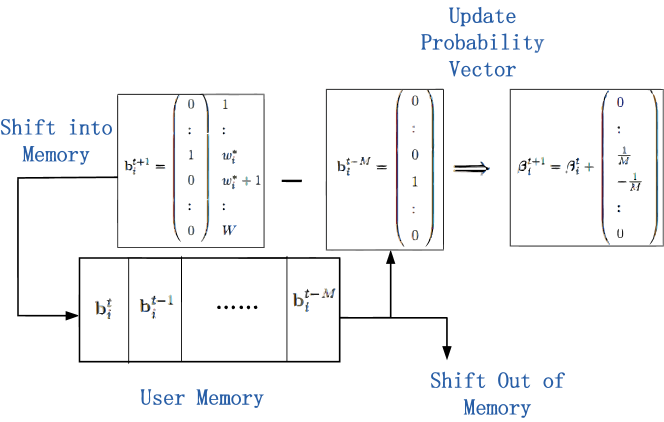
Remark 3
In step 4) of JASPA, each MU’s probability vector is updated. A graphical illustration of this step for user is provided in Fig. 1. By following the update rule in (25), the -th entry of will be at least over the next iterations. This step combined with the randomization procedure in step 5) ensure that all of MU ’s best AP in the most recent iterations have the probability of at least of being selected as . This is in contrast to a naive greedy strategy that always selects the best AP for the MUs in every iteration. In fact, such greedy algorithm may diverge 333Indeed, a simple example of the divergence of the greedy algorithm is in a AP user network, in which each AP has a single channel. Suppose the users’ channels are all identical, and both users associate with the same AP at the beginning. Then each of them will always perceive the vacant AP as its “best AP”. Each of them will then switch back and forth between the APs and will never stabilize. , while the proposed randomized selection algorithm guarantees convergence (see Theorem 3.)
Remark 4
To avoid unnecessary overhead related to ending and establishing the connections, it is reasonable to assume that a selfish MU is willing to leave its current AP only if the new AP can offer significant improvement of the data rate. To model such behavior, we introduce a connection cost for each MU. Then the set should contain the APs that satisfy the following inequality
From a system point of view, introducing these connection costs may improve the convergence speed of the algorithm, as the MUs are less willing to change associations. However it might also result in reduced system throughput.
Remark 5
Suppose at time , the algorithm terminates with profile . Then must be a NE association profile. To see this, note that the algorithm stops when appears in consecutive iterations. From the way that the actual AP association is generated, we see that during iterations , each MU must prefer at least once. More precisely, must be preferred by all the MUs in the system. It follows that is an equilibrium solution.
The following theorem shows that the JASPA converges to a JEP globally regardless of the starting points or the realizations of the channel gains. See Appendix IX-B for proof.
Theorem 3
When choosing , the JASPA algorithm produces a sequence that converges to a JEP with probability 1.
V Extensions to the JASPA Algorithm
The JASPA algorithm presented in the previous section is “distributed” in the sense that the computation in each iteration can be performed locally by the MUs. However, it requires the MUs to jointly implement an intermediate power equilibrium between two AP selections and , which entails significant coordination among the MUs. In this section, we propose two extensions of the JASPA algorithm that do not require the MUs to reach any intermediate equilibria.
The first algorithm, named Se-JASPA, is a sequential version of the JASPA. It is detailed in Table II.
| 1) Initialization: Each MU randomly chooses and |
| 2) Determine the Next AP Association: |
| If it is MU ’s turn to act, (e.g., ): |
| 2a) MU finds a set that satisfies |
| 2b) MU selects an AP by randomly picking . |
| For other MUs , . |
| 3) Update the Power Allocation: |
| Denote . MU updates by . |
| For other MUs , . |
| 4) Continue: Let t=t+1, and go to Step 2) |
The Se-JASPA algorithm differs from the original JASPA algorithm in several important ways. Firstly, each MU does not need to record the history of its best-reply vectors . It decides on its AP association greedily in step 2). Secondly, a MU , after deciding a new AP , does not need to go through the process of reaching an intermediate equilibrium. However, the MUs still need to be coordinated for the exact sequence of their update, because in each iteration only a single MU is allowed to act. As can be inferred by the sequential nature of this algorithm, when the number of MUs is large, the convergence becomes slow.
An alternative simultaneous version of the algorithm (named Si-JASPA) is listed in Table III. Differently from the Se-JASPA algorithm, it allows for all the users to update in each iteration. We note that in the algorithm, the variable represents the duration that MU has stayed in the current AP; the sequence of stepsizes is chosen according to (10).
| 1) Initialization (t=0): |
| Each MU randomly chooses and |
| 2) Selection of the Best Reply Association: |
| Each MU computes following Step 3) of JASPA |
| 3) Update Probability Vector: |
| Each MU updates according to (25) |
| Push into the memory; |
| Remove from the memory if |
| 4) Determine the Next AP Association: |
| Each MU obtains following Step 5) of JASPA |
| 5) Compute the Best Power Allocation: |
| Let ; |
| Each MUs calculates by |
| 6) Update the Duration of Stay: |
| Each MU maintains and updates a variable : |
| 7) Update the Power Allocation: |
| Each MU calculates as follows: |
| 8) Continue: Let t=t+1, and go to Step 2) |
The structure of the Si-JASPA is almost the same as the JASPA, except that for each MU, after switching to a new AP, it does not need to go through the process of joint computation of the intermediate equilibrium. Instead, the MUs can make their AP decisions in each iteration of the algorithm. The level of coordination among the MUs required for this algorithm is minimum among all the three algorithms introduced so far.
Although to this point there is no complete convergence results for the Se/Si-JASPA algorithms, our simulations suggest that they indeed converge. Moreover, the Si-JASPA usually converges faster than the Se-JASPA.
VI JASPA Based on Network-Wide Joint-Strategy
In this section, an alternative algorithm with convergence guarantee is proposed. This algorithm allows the MUs, as in the Se/Si-JASPA, to jointly select their power profiles and AP associations without the need to reach any intermediate equilibria. We will see later that compared with the JASPA and its two variants introduced before, the algorithm studied in this section requires considerably different information/memory structure for the MUs and the APs. Among others, it requires that the MUs maintain in their memory the history of some network-wide joint strategy of all MUs. We henceforth name this algorithm the Joint-strategy JASPA (J-JASPA).
VI-A The J-JASPA Algorithm
The main idea of the J-JASPA algorithm is to let the MUs compute their strategies according to some system state that is randomly sampled from the history. This is different from the JASPA and Si-JASPA algorithm, in which the MUs compute their best strategies according to the current system state, but then perform their actual association by random sampling the history of the best strategies. To better introduce the proposed algorithm, we first provide some definitions.
-
•
Let denotes the set of MUs that are associated with AP in iteration .
-
•
Let be the joint interference profile of the set of MUs .
We then elaborate on the required memory structure. Let each MU keep three different kinds of memories, each with length and operates in a FIFO fashion.
-
1.
The first memory, denoted as , records MU ’s associated APs in the last iterations: , i.e., , for .
-
2.
The second memory, denoted as , records the MU ’s interference levels in the last iterations, , where . That is, , for .
-
3.
The third memory, denoted as , records MU ’s rate in the last iterations, .
Each AP is also required to keep track of some local quantities 444Here, “local” means individual APs can gather these pieces of information without the need to communicate with other APs. related to the history of the MUs’ behaviors. Suppose a subset of users has been associated with AP at least once during iterations . Let us define the time index as the most recent time index that appears in AP . The following variables are required to be recorded by each AP :
-
•
The local power profile .
-
•
The local interference profile .
-
•
The total number of times that has appeared in AP : , where is the indicator function.
The J-JASPA algorithm is stated as follows:
1) Initialization: Let , each MU randomly chooses
and
.
2) Update MU Memory: For each , obtain
from the APs. If , Remove
, and
. Push ,
, and
into the end of ,
and , respectively.
3) Update AP Memory: For each , perform the
following updates:
4) Sample Memory: Let , and let be the all vector. Each MU samples its memories by:
Set , and .
5) The Best AP Association: Each MU computes the set of best APs by the sampled variables , and :
| (26) |
Randomly pick , and set
.
6) The Power Allocation: Each MU switches to AP
. MU obtains
,
, and
from
AP .
If , then let and . Choose power according to
| (27) |
Else randomly pick
.
7) Continue: Let , go to step 2).
Comparing with the JASPA and Si-JASPA algorithms, the J-JASPA algorithm possesses the following distinctive features.
-
1.
In J-JASPA, each MU calculates its best AP association according to a sampled historical network state, while in the JASPA and Si-JASPA, it calculates this quantity according to the current network state.
-
2.
The J-JASPA algorithm requires the APs to have memory. Each AP needs to record the local power allocation and interference profiles for all the different sets of MUs that have been associated with it in the previous iterations. No such requirement is imposed on all the previously introduced algorithms.
-
3.
The J-JASPA requires larger memory for the MUs for constructing , and .
-
4.
The J-JASPA requires extra communications between the MUs and the APs. Such overhead mainly comes from step 6), in which the MUs retrieve information stored in the APs for their power updates.
VI-B The convergence of the J-JASPA algorithm
In this subsection, we show that the J-JASPA algorithm converges to a JEP. The proofs of the claims made in this subsection can be found in Appendix IX-C to IX-E
Let a set consist of association profiles that appear infinitely often in the sequence . We first provide a result related to the power allocation along an infinite subsequence in which appears.
Proposition 2
Choose . Let be a subsequence such that . Then for all , , which is an optimizer of the problem . Furthermore, we have that and
We need the following definitions to proceed. Let be the profile sampled from the memory by the MUs in step 4) at time : . For a specific , let the subsequence be the time instances that appears and is immediately sampled by all the MUs, i.e., . Note that if , then according to step 3)-step 4), with non-zero probability, . Thus, if , then is an infinite sequence.
Define as the maximum rate MU can achieve in AP based on the interference . Define MU ’s best association set as:
| (28) |
where is the sampled rate given in step 4). From step 5) of the J-JASPA algorithm, all has non-zero probability to be the serving AP for MU in iteration . Let . Due to Proposition 2, and the fact that appears infinitely often, such limit is well defined. Next we provide an asymptotic characterization of the best association set defined above.
Proposition 3
For a specific MU and a system association profile , suppose there exists a such that , i.e., MU has the incentive to move to a different AP in the limit. Then there exists a large enough constant such that for all , we have:
| (29) |
In words, when a profile appears infinitely often, and suppose in the limit, when is sampled, a MU prefers . Then it must prefer in every time instance when is large enough. Now we are ready to provide the main convergence result for the J-JASPA algorithm.
Theorem 4
When choosing , the J-JASPA algorithm converges to a JEP with probability 1.
VII Simulation Results
In this section, we demonstrate the performance of the JASPA algorithm and its three variants discussed in this work. The following simulation setting is considered. Multiple MUs and APs are randomly placed in a by area. We use to denote the distance between MU and AP . Unless otherwise noted, the channel gains between MU and AP are generated independently from an exponential distribution with mean (i.e., is assumed to have Rayleigh distribution). Pre-assign the available channels equally to different APs. Throughout, a snapshot of the network refers to the network with fixed (but randomly generated as above) AP, MU locations and channel gains. The length of the individual memory is set as . For ease of comparison, when we use the JASPA algorithm with connection cost, we set all the MUs’ connection cost to be identical.
We first show the results related to the convergence properties, and then present the results related to the system throughput performance. Due to the space limit, for each experiment we show the results obtained by running either Si/Se-JASPA and J-JASPA, or those obtained by the JASPA.
VII-1 Convergence
Only the the results for Si/Se-JASPA and J-JASPA are shown in this subsection. We first consider a network with MUs, channels, and APs. Fig. 2 shows the evolution of the system throughput as well as the system potential function generated by a typical run of the Se-JASPA, Si-JASPA, J-JASPA and Si-JASPA with connection cost bit/sec . We observe that the Si-JASPA with connection cost converges faster than Si-JASPA and Se-JASPA, while Se-JASPA converges very slowly. After convergence, the system throughput achieved by Si-JASPA with connection cost is smaller than those achieved by the other three algorithms.
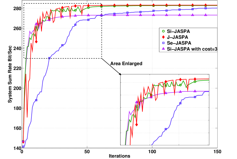
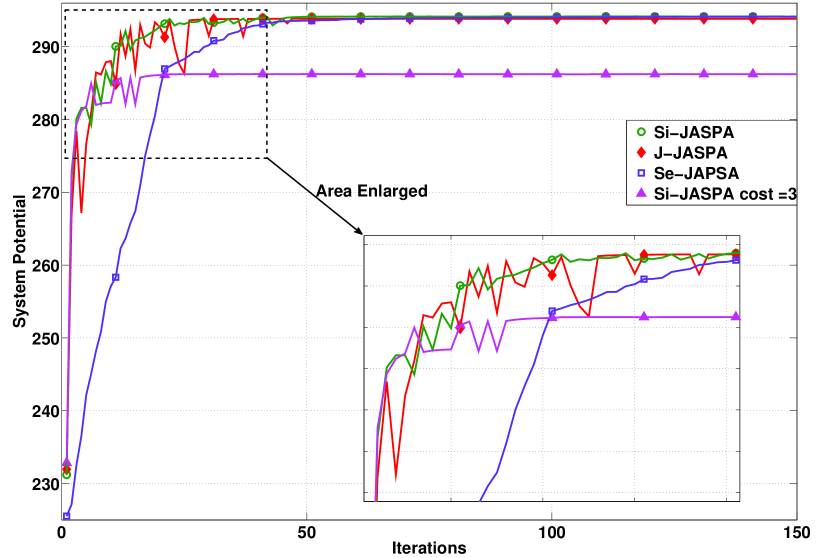
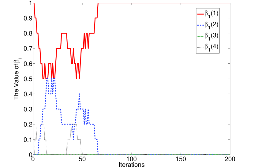
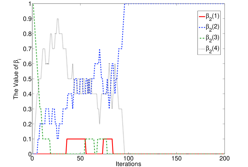
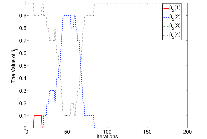
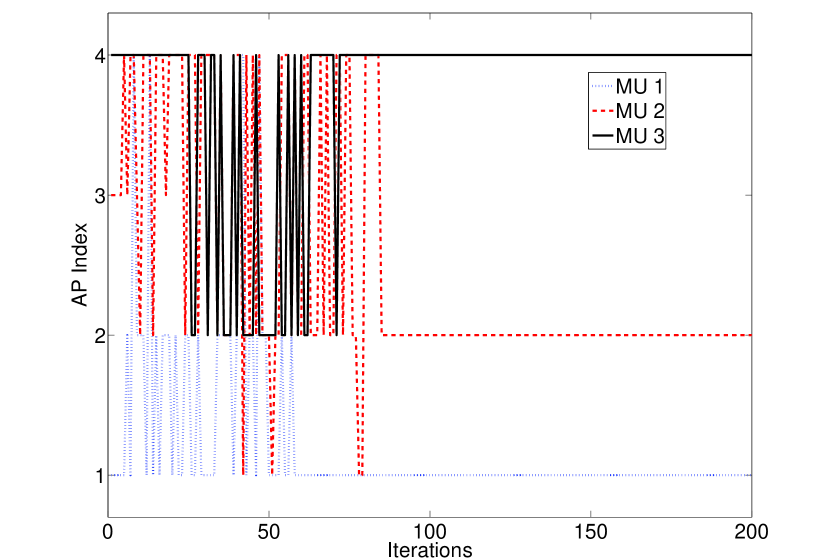
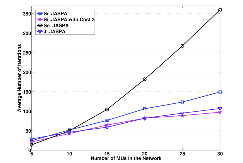
Fig. 5 shows the evolution of the AP selections made by the MUs in the network during a typical run of the Si-JASPA algorithm. We only show 3 out of 20 MUs (the selected MUs are labeled as MU 1, 2, 3 for easy reference) in order not to make the figure overly crowded. Fig. 3 shows the corresponding evolution of the probability vectors for the three of the MUs selected in Fig. 5. It is clear that upon convergence, all the probability vectors converge to unit vectors. Fig. 5 evaluates the impact of the number of MUs on the speed of convergence of different algorithms. When becomes large, the sequential version of the JASPA takes significantly longer time to converge than the other three simultaneous versions of the algorithm. Moreover, the J-JASPA exhibits faster convergence than the Si/Se-JASPA. It is also noteworthy to mention that including the connection costs indeed helps to accelerate the convergence for the algorithm.
VII-2 System Throughput Performance
We evaluate the throughput achievable by the JEP computed by the JASPA. Such throughput performance is compared against a simple baseline algorithm that assigns the users to their closest AP in terms of actual distance. After assignment, the power allocation is computed using the A-IWF algorithm discussed in Section II.
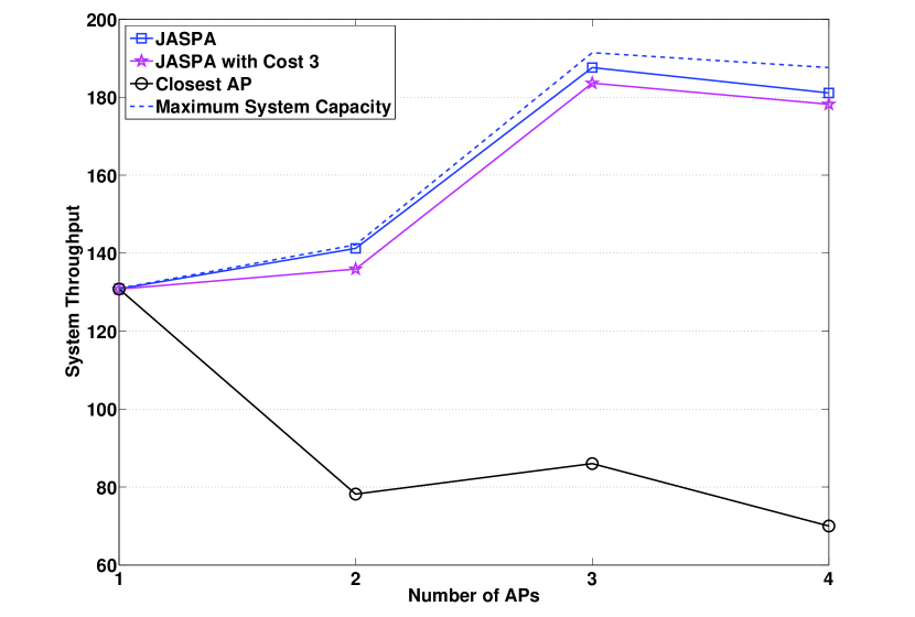
We first consider a small network with MUs, channels and APs. We compare the performance of the JASPA algorithms to the maximum throughput that can be achieved. The maximum throughput for a snapshot of the network is calculated by an exhaustive search procedure: 1) for a given association profile, say , calculate the maximum throughput (denoted by ) by summing up the maximum achievable rate of all APs in the network; 2) enumerate all possible association profiles, and find .
In Fig. 7, we see that the JASPA algorithm performs very well with little throughput loss, while the closest AP algorithm performs poorly. We then investigate the performance of larger networks with 30 MUs, up to 16 APs and up to 128 channels. Fig. 7 shows the comparison of the performance of JASPA, JASPA with individual cost bit/sec and bit/sec.
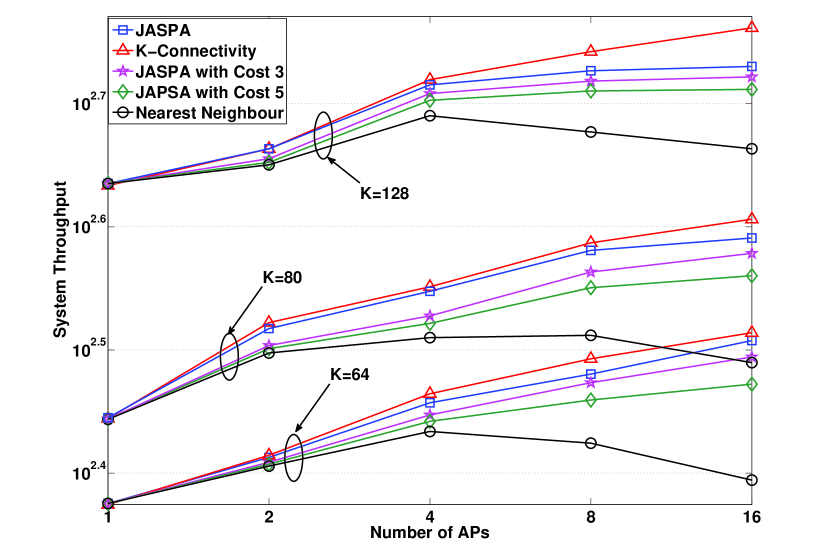
Due to the prohibitive computation time required, we are unable to obtain the maximum system throughput for these relatively large networks. For comparison purpose, we instead compute the equilibrium system throughput that can be achieved in a game if all the MUs are able to connect to all the APs at the same time. In such ideal network, all the APs are pooled together as a single “virtual” AP, which along with the users form a “virtual” MAC channel. The users can allocate their transmit power by computing the NE for the corresponding single AP game, as discussed in Section II. As suggested in Section II-B, when the number of channel becomes large, the throughput achieved by the NE of this power allocation game achieves the capacity of the “virtual” MAC. However, we observe that the performance of JASPA is close to that of such ideal “multiple-connectivity” network.
VIII Conclusion
In this paper, we addressed the joint AP selection and power allocation problem in a multichannel wireless network. The problem was formulated as a non-cooperative game with mixed-integer strategy space. We characterized the NEs of this game, and provided distributed algorithms to reach the NEs. Empirical evidence gathered from simulation suggests that the quality of the equilibrium solutions is reasonably high.
There can be many future extensions to this work. First of all, the non-cooperative game with mixed-integer strategy space analyzed in this paper can be applied to many other problems as well, for example, the downlink counterpart of the current problem. Secondly, for the problem considered in this work, it is beneficial to characterize quantitatively the efficiency of the JEP, and to provide solutions for efficiency improvement. Thirdly, it would be interesting to investigate the effect of time-varying channels and the arrival and departure of the MUs on the performance of the algorithm.
IX Appendix
IX-A Proof of Proposition 1
Note that the WF operator is also a function of , hence we can rewrite it as . Define . Define . Then the A-IWF algorithm can be expressed as:
We first state and prove two lemmas.
Lemma 1
We have , where and are two constants.
Proof:
To prove the first inequality, we need to show that:
| (30) |
where . It suffices to show that for each , there exists such that:
| (31) |
Expressing explicitly, we have
| (32) |
Note that the Lagrangian multiplier ensures the tightness of MU ’s power budget constraint. Therefore we must have , which in turn implies:
| (33) |
Define two index sets , . Then each inequality in (31) is equivalent to
| (34) |
From (33) we have . Using this result, we see that to show (34), it suffices to show that there exists such that:
| (35) |
Pick any , . Below we will show that for the pair there exists such that:
| (36) |
Note that if (36) is true, we can take , then (35) is true, which in turn implies (31).
In the following, we prove (36) for any pair with and .Let us first simplify the term by denoting , where . We can verify that:
| (37) |
Similarly, the term can be simplified as . In this case, we have:
| (38) |
Due to (37) and (38), in order to prove (36), it suffices to prove that there exists such that:
| (39) |
Notice that from the definition, for any we have . Then the above inequality can be simplified to:
| (40) |
From (37) and (38) we have that and . Therefore we must have . Consequently, (40) is equivalent to Finding such is always possible, as is bounded away from 0 for any (cf. (32), and note and ).
Now that we can always find a constant that satisfies (36), we can take to ensure (31). Thus, taking , (30) is true, and the first part of the proposition is proved.
The second part of the proposition is straightforward. Due to space limit, we do not show the proof here. ∎
Lemma 2
For two vectors and , there must exist constants , such that
Proof:
First note that if for all , there exists a constant , such that: , then the first inequality in the lemma is true for . Define a vector where its th element is given as ; let denote the projection to the feasible set . Then from [26, Lemma 1], we have that . Notice that we have
| (41) |
where . Then we have that
| (42) |
where is because of the triangular inequality and the non-expansiveness of the Euclidean norm. Thus, taking , we have that .
The second inequality in the Lemma can be shown similarly. ∎
Using Lemma 1 and Lemma 2, Proposition 1 can be shown by slightly generalizing the existing result [27, Proposition 3.5], which proves the convergence for a family of gradient methods with diminishing stepsizes for unconstrained problems. The generalization of this cited result to the current constrained case is to some extent straightforward, and we omit the proof due to space limitations.
IX-B Proof of Theorem 3
We first introduce some notations. Define a vector such that if then . Define a set as: .
Step 1): We first show that there must exist a NE association profile . Let us pick any . Suppose is not a NE association profile, and in iteration , .
From step 3) of the JASPA, for a specific MU , all the APs must satisfy (24). From step 2) of the algorithm, for AP , we have . From Corollary 2, we have that must be a NE for the single AP power allocation game with the set of players . Utilizing the definition of the NE in (5), we must have
That is, . From step 3) of the algorithm, we see that each , in particular , has the probability of of being selected as . From step 4)–step 5) of the algorithm, we see that with probability at least . It follows that
| (43) |
Suppose is not a NE, then there must exist a MU such that there is an AP that satisfies and
Following the same argument as in the previous paragraph, we have . It follows that
| (44) |
The proof of Theorem 2 suggests that if a single MU switches to an AP that increases its rate, then the system potential increases. In our current context, this says if , then .
Starting from iteration , with positive probability, in each iteration a single MU switches to its preferred AP. The potentials generated in this way is strictly increasing. This process, however, will stop at a finite time index such that no MU is willing to switch. Consequently, is an equilibrium association profile. The finiteness of is from the finiteness of distinctive association profiles (and hence the finiteness of possible values for ). Such finiteness combined with the fact that each step of of the above process happens with non-zero probability imply that the probability of reaching from is non-zero.
We conclude that with non-zero probability, a NE profile will appear after in finite steps. Combined with the assumption that appears infinitely often, we must also have that .
Step 2): We can then show that the sequence converges to an equilibrium profile . This step can be shown using the same argument as in [1, Theorem 2]. Due to space limitation, we choose not to reproduce the proof here.
IX-C Proof of Proposition 2
Proof:
For a , let . Let be a subsequence in which the subset of MUs is associated with AP . Clearly, is a subsequence of . From the J-JASPA algorithm, we see that at each , (27) implements the single AP A-IWF algorithm with the fixed set of MUs . Therefor, Proposition 1 implies that the subsequence (consequently ) converges to , an optimizer of the problem . From Corollary 2 and the fact that for all , we obtain and . ∎
IX-D Proof of Proposition 3
Proof:
From Proposition 2, we have that for a given , , which implies that and . The latter equality combined with the continuity of the rate function with respect to , and the continuity of the function with respect to , further implies that, for any , there must be a constant such that for all , the following are true:
| (45) |
For any satisfying , there must exit a such that:
| (46) |
Take , choose a constant satisfying , and let . For simplicity of notation, write instead of . We have that for all , the following is true:
| (47) |
Consequently, we have that for all , which implies that must be in the set . The claim is proved. ∎
IX-E Proof of Theorem 4
Proof:
Consider the sequence . Choose to be any system association profile that satisfies: Again let . From Proposition 2 we have that the sequence converges, i.e., . We first show that is a JEP.
Suppose is not a JEP, then there exists a MU , and a such that . This implies that there exists an such that:
| (48) |
Define a new association profile . Following the similar steps as in the proof of Theorem 2, we can show that: . It is clear that if , then the previous inequality is a contradiction to the assumption that . In the following, we show that , which completes the proof.
From Proposition 3, there exists a large enough that for all , . Take any . From the definition, in iteration , is sampled, that is, . From step 5) of the J-JASPA algorithm, we see that with non-zero probability, in iteration , all MUs stay in , and MU chooses to switch to . This implies that the association profile happens with non-zero probability in every time instance . Because is an infinite sequence, happens infinitely often, i.e., .
In summary, we conclude that must be a NE association profile, and thus, is a JEP.
Finally, following the proofs of Theorem 3, we can show similarly that the sequence generated by the J-JASPA converges to a JEP with probability 1. ∎
References
- [1] M. Hong, A. Garcia, and J. Barrera, “Joint distributed AP selection and power allocation in cognitive radio networks,” in the Proceedings of the IEEE INFOCOM, 2011.
- [2] C. R. Stevenson, G. Chouinard, Z. Lei, W. Hu, S. J. Shellhammer, and W. Caldwell, “IEEE 802.22: the first cognitive radio wireless regional area network standard,” Comm. Mag., vol. 47, no. 1, pp. 130–138, 2009.
- [3] J. Acharya and R. D. Yates, “Dynamic spectrum allocation for uplink users with heterogeneous utilities,” IEEE Transactions on Wireless Communications, vol. 8, no. 3, pp. 1405–1413, 2009.
- [4] D. Niyato and E. Hossain, “Call admission control for QoS provisioning in 4G wireless networks: issues and approaches,” IEEE Network, vol. 19, no. 5, pp. 5 – 11, 2005.
- [5] J. McNair and F. Zhu, “Vertical handoffs in fourth-generation multinetwork environments,” IEEE Wireless Communications, vol. 11, no. 3, pp. 8 – 15, 2004.
- [6] T. Alpcan and T. Basar, “A hybrid noncooperative game model for wireless communications,” Annals of the International Society of Dynamic Games, vol. 9, pp. 411–429, 2007.
- [7] C. U. Sarayda, N. B. Mandayam, and D. J. Goodman, “Pricing and power control in a multicell wireless data network,” IEEE Journal on selected areas in communications, vol. 19, no. 10, pp. 1883–1892, 2001.
- [8] L. Lai and H. E. Gamal, “The water-filling game in fading multiple-access channels,” IEEE Transactions on Information Theory, vol. 54, no. 5, 2008.
- [9] G. He, S. Gault, M. Debbah, and E. Altman, “Distributed power allocation game for uplink OFDM systems,” in Proc. WiOPT, 2008, pp. 515–521.
- [10] W. Yu, W. Rhee, S. Boyd, and J. M. Cioffi, “Iterative water-filling for Gaussian vector multiple-access channels,” IEEE Transactions on Information Theory, vol. 50, no. 1, pp. 145–152, 2004.
- [11] S. V. Hanly, “An algorithm for combined cell-site selection and power control to maximize cellular spread spectrum capacity,” IEEE Journal on selected areas in communications, vol. 13, pp. 1332–1340, 1995.
- [12] R. D. Yates and C. Y. Huang, “Integrated power control and base station assignment,” IEEE Transactions on Vehicular Technology, vol. 44, pp. 1427–1432, 1995.
- [13] F. Meshkati, M. Chiang, H. V. Poor, and S. C. Schwartz, “A game-theoretic approach to energy-efficient power control in multicarrier CDMA systems,” IEEE Journal on Selected Areas in Communications, vol. 24, pp. 1115–1129, 2006.
- [14] S. Shakkottai, E. Altman, and A. Kumar, “Multihoming of users to access points in WLANs: A population game perspective,” IEEE Journal on Selected Areas In Communications, pp. 1207–1215, August 2007.
- [15] A. Leshem and E. Zehavi, “Game theory and the frequency selective interference channel,” IEEE Sig. Process. Mag., vol. 26, no. 5, 2009.
- [16] “Special section on game theory in signal processing and communications,” sept 2009, IEEE Signal Processing Magazine.
- [17] M. Hong and Z.-Q. Luo, “Signal processing and optimal resource allocation for the interference channel,” EURASIP E-Reference Signal Processing, 2012, accepted, available at http://arxiv.org.
- [18] T. M. Cover and J. A. Thomas, Elements of Information Theory, second edition, Wiley, 2005.
- [19] Z. Q. Luo and S. Z. Zhang, “Dynamic spectrum management: Complexity and duality,” IEEE Journal of Selected Topics in Signal Processing, vol. 2, no. 1, pp. 57–73, 2008.
- [20] M. J. Osborne and A. Rubinstein, A Course in Game Theory, MIT Press, 1994.
- [21] D. Monderer and L. S. Shapley, “Potential games,” Games and Economics Behaviour, vol. 14, pp. 124–143, 1996.
- [22] G. Scutari, S. Barbarossa, and D. P. Palomar, “Potential games: A framework for vector power control problems with coupled constraints,” in the Proceedings of ICASSP 06, 2006.
- [23] S. Ohno, G. B. Giannakis, and Z.-Q. Luo, “Multicarrier multiple access is sum-rate optimal for block transmissions over circulant ISI channels,” in in Proc. IEEE Conference on Communications, 2002, pp. 1656–1660.
- [24] M. Hong and A. Garcia, “Averaged iterative water-filling algorithm: Robustness and convergence,” IEEE Transactions on Signal Processing, vol. 59, no. 5, pp. 2448 –2454, may 2011.
- [25] P. Mertikopoulos, E. V. Belmega, A. L. Moustakas, and S. Lasaulce, “Dynamic power allocation games in parallel multiple access channels,” in Proceedings of the 5th International ICST Conference on Performance Evaluation Methodologies and Tools, ICST, Brussels, Belgium, Belgium, 2011, pp. 332–341.
- [26] G. Scutari, D. P. Palomar, and S. Barbarossa, “Optimal linear precoding strategies for wideband noncooperative systems based on game theory – part II: Algorithms,” IEEE Transactions on Signal Processing, vol. 56, no. 3, 2008.
- [27] D. P. Bertsekas and J. N. Tsitsiklis, Neuro-Dynamic Programming, Athena Scientific, Belmont, MA, 1996.