Equivalence between Priority Queues and Sorting in External Memory

A priority queue is a fundamental data structure that maintains a dynamic ordered set of keys and supports the followig basic operations: insertion of a key, deletion of a key, and finding the smallest key. The complexity of the priority queue is closely related to that of sorting: A priority queue can be used to implement a sorting algorithm trivially. Thorup [10] proved that the converse is also true in the RAM model. In particular, he designed a priority queue that uses the sorting algorithm as a black box, such that the per-operation cost of the priority queue is asymptotically the same as the per-key cost of sorting. In this paper, we prove an analogous result in the external memory model, showing that priority queues are computationally equivalent to sorting in external memory, under some mild assumptions. The reduction provides a possibility for proving lower bounds for external sorting via showing a lower bound for priority queues.

1 Introduction

The priority queue is an abstract data structure of fundamental importance. A priority queue maintains a set of keys and support the following operations: insertion of a key, deletion of a key, and findmin, which returns the current minimum key in the priority queue. It is well known that a priority queue can be used to implement a sorting algorithm: we simply insert all keys to be sorted into the priority queue, and then repeatedly delete the minimum key to extract the keys in sorted order. Thorup [10] showed that the converse is also true in the RAM model. In particular, he showed that given a sorting algorithm that sorts $N$ keys in $NS(N)$ time, there is a priority queue that uses the sorting algorithm as a black box, and supports insertion and deletion in $O(S(N))$ time, and findmin in constant time. The reduction uses linear space. The main implication of this reduction is that we can regard the complexity of internal priority queues as settled, and just focus on establishing the complexity of sorting. Algorithmically, it also gives new priority queue constructions by using the fastest (integer) sorting algorithms currently known: an $O(N\log\log N)$ deterministic algorithm by Han [6] and an $O(N\sqrt{\log\log N})$ randomized one by Han and Thorup [7].

In this paper, we prove an analogous result in the external memory model (the I/O model), showing that priority queues are almost computationally equivalent to sorting in external memory. We design a priority queue that uses the sorting algorithm as a black box, such that the update cost of the priority queue is essentially the same as the per-key I/O cost of the sorting algorithm. The priority queue always has the current minimum key in memory so findmin can be handled without I/O cost. Our priority queue is a non-trivial generalization of Thorup’s, which is fundamentally an internal structure. The main reasons why Thorup’s structure does not work in the I/O model are that it cannot flush the buffers I/O-efficiently, and that it does not specify any order for performing the flush and rebalance operations. Moreover, deletions are supported in a very different way in the I/O model; we have to do it in a lazy fashion in order to achieve I/O-efficiency.

1.1 Our results

Let us first recall the standard I/O model [1]: The machine consists of an internal memory of size $M$ and an infinitely large external memory. Computation can only be carried out in internal memory. The external memory is divided into blocks of size $B$, and data is moved between internal and external memory in terms of blocks. We measure the complexity of an algorithm by counting the number of I/Os it performs, while internal memory computation is free.

Our main result is stated in the following theorem:

Theorem 1.1.

Suppose we can sort up to $N$ keys in $NS(N)/B$ I/Os in external memory, where $S$ is a non-decreasing function. Then there exists an external priority queue that uses linear space and supports a sequence of $N$ insertion and deletion operations in $O(\frac{1}{B}\sum_{i\geq 0}S(B\log^{(i)}\frac{N}{B}))$ amortized I/Os per operation. Findmin can be supported without I/O cost. The reduction uses $O(B)$ internal memory and is deterministic.

The first implication of Theorem 1.1 is that if the main memory has size $\Omega(B\log^{(c)}\frac{N}{B})$ for any constant $c$, then our priority queue supports insertion and deletion with $O(S(N)/B)$ amortized I/O cost. This is because $S(N)=0$ when $N\leq M$. Even if $M=O(B)$, the reduction is still tight as long as the function $S$ grows not too slowly. More precisely, we have the following corollary:

Corollary 1.2.

For $S(N)=\Omega(2^{\log^{*}\frac{N}{B}})$, the priority queue supports updates with $O(S(N)/B)$ amortized I/O cost; for $S(N)=o(2^{\log^{*}\frac{N}{B}})$, the priority queue supports updates with $O(S(N)\log^{*}\frac{N}{B}/B)$ amortized I/O cost.

The first part can be verified by plugging $S(N)=2^{\log^{*}\frac{N}{B}}$ into Theorem 1.1 and showing that the $S(B\log^{(i)}\frac{N}{B})$’s decrease exponentially with $i$. For the second part, we simply relax all the $S(B\log^{(i)}\frac{N}{B})$’s to $S(N)$. Note that $2^{\log^{*}\frac{N}{B}}=o(\log^{(c)}\frac{N}{B})$ for any constant $c$, so it is very unlikely that a sorting algorithm could achieve $S(N)=o(2^{\log^{*}\frac{N}{B}})$. No such algorithm is known, even in the RAM model. Therefore, we can essentially consider our reduction to be tight.

1.2 Related work

Sorting and priority queues have been well studied in the comparison-based I/O model, in which the keys can only be accessed via comparisons. Aggarwal and Vitter [1] showed that $\Theta(\frac{N}{B}\log_{M/B}\frac{N}{B})$ I/Os are sufficient and necessary to sort $N$ keys in the comparison-based I/O model. This bound is often referred to as the sorting bound. If the comparison constraint is replaced by the weaker indivisibility constraint, there is an $\Omega(\min\{\frac{N}{B}\log_{M/B}\frac{N}{B},N\})$ lower bound, known as the permuting bound. The two bounds are the same when $\frac{N}{B}\log_{M/B}\frac{N}{B}<N$; it is conjectured that for this parameter range, $\Omega(\frac{N}{B}\log_{M/B}\frac{N}{B})$ is still the sorting lower bound even without the indivisibility constraint. For $\frac{N}{B}\log_{M/B}\frac{N}{B}>N$, the current situation in the I/O model is the same as that in the RAM model, that is, the best upper bound is just to use the best RAM algorithm (which has $O(N\log\log N)$ time deterministically or $O(N\sqrt{\log\log N})$ time randomized) naively in external memory ignoring the blocking at all, and there is no non-trivial lower bound. When the block size is not too small, none of the RAM sorting algorithms works better than the comparison-based one, which makes the situation “cleaner”. Thus, a sorting lower bound (without any restrictions) has been considered to be more hopeful in the I/O model (with $B$ not too small) than in the RAM model, and it was posed as a major open problem in [1]. Thus, our result provides a way to approach a sorting lower bound via that of priority queues, while data structure lower bounds have been considered (relatively) easier to obtain than (concrete) algorithm lower bounds (except in restricted computation models), as witnessed by the many recent strong cell probe lower bounds for data structures, such as [9, 8] among many others. However, our result does not offer any new bounds for priority queues because we do not know of a better sorting algorithm than the comparison-based ones in the I/O model (and the conjecture is that they do not exist when $\frac{N}{B}\log_{M/B}\frac{N}{B}<N$).

Since a priority queue can be used to sort $N$ keys with $N$ insertion and $N$ deletemin operations, it follows that $\Omega(\frac{1}{B}\log_{M/B}\frac{N}{B})$ is also a lower bound for the amortized I/O cost per operation for any external priority queue, in the comparison-based I/O model. There are many priority queue constructions that achieve this lower bound, such as the buffer tree [2], $M/B$-ary heaps [5], and array heaps [4]. See the survey [11] for more details. However, they do not use sorting as just a black box, and cannot be improved even if we have a faster external sorting algorithm. Thus they do not give a priority queue-to-sorting reduction. The extra $O(\log_{M/B}\frac{N}{B})$ factor comes from a tree structure with fanout $O(M/B)$ within the priority queue construction. and a key must be moved $\Omega(\log_{M/B}\frac{N}{B})$ times to “bubble up” or “bubble down”.

Arge et al. [3] developed a cache-oblivious priority queue that achieves the sorting bound with the tall cache assumption, that is, $M$ is assumed to be of size at least $B^{2}$. We note that their structure can serve as a priority queue-to-sorting reduction in the I/O model, by replacing the cache-oblivious sort with a sorting black box. The resulting priority queue supports all operations in $O(\frac{1}{B}\sum_{i\geq 0}S(N^{(2/3)^{i}})$ amortized I/Os if the sorting algorithm sorts $N$ keys in $NS(N)/B$ I/Os. However, this reduction is not tight for $S(N)=O(\log\log\frac{N}{B})$, and there seems to be no easy way to get rid of the tall cache assumption, even if the algorithm has the knowledge of $M$ and $B$.

2 Structure

In this section, we describe the structure of our priority queue. In the next section, we show how this structure supports various operations. Finally we analyze the I/O costs of these operations.

The priority queue consists of multiple layers whose sizes vary from $N$ to $cB$, where $c$ is some constant to be determined later. The $i$’th layer from above has size $\Theta(B\log^{(i)}\frac{N}{B})$, for $i\geq 0$, and the priority queue has $O(\log^{*}N)$ layers. For the sake of simplicity we will refer to a layer by its size. Thus the layers from the largest to the smallest are layer $N$, layer $B\log\frac{N}{B}$, $\ldots$, layer $cB$. Layer $cB$ is also called head, and is stored in main memory. Given a layer $X$, its upper layer and lower layer are layer $B2^{\frac{X}{B}}$ and layer $B\log\frac{X}{B}$, respectively. We use $\Psi_{X}$ to denote $B2^{\frac{X}{B}}$ and $\Phi_{X}$ to denote $B\log\frac{X}{B}$. The priority queue maintains the invariant that the keys in layer $\Phi_{X}$ are smaller than the keys in layer $X$. In particular, the minimum key is always stored in the head and can be accessed without I/O cost.

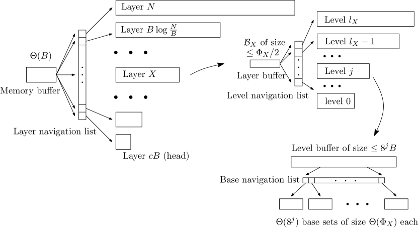
Figure 1: The components of the priority queue.

We maintain a main memory buffer of size $O(B)$ to accommodate incoming insertion and deletion operations. In order to distribute keys in the memory buffer to different layers I/O-efficiently, we maintain a structure called layer navigation list. Since this structure will also be used in other components of the priority queue, we define it in a unified way. Suppose we want to distribute the keys in a buffer $\mathcal{B}$ to $t$ sub-structures $S_{1},S_{2},\ldots S_{t}$. The keys in different sub-structures are sorted relative to each other, that is, the keys in $S_{i}$ are less or equal to the keys in $S_{i+1}$. Each sub-structure $S_{i}$ is associated with a buffer $\mathcal{B}_{i}$, which accommodates keys transferred from $\mathcal{B}$. The goal is to distribute the keys in $\mathcal{B}$ to each $\mathcal{B}_{i}$ I/O-efficiently, such that the keys that go to $\mathcal{B}_{i}$ have values between the minimum keys of $S_{i}$ and $S_{i+1}$. A navigation list stores a set of $t$ representatives, each representing a sub-structure. The representative of $S_{i}$, denoted $r_{i}$, is a triple that stores the minimum key of $S_{i}$, the number of keys stored in $\mathcal{B}_{i}$, and a pointer to the last non-full block of the buffer $\mathcal{B}_{i}$. The representatives are stored consecutively on the disk, and are sorted on the minimum keys. The layer navigation list is built for the $O(\log^{*}N)$ layers, so it has size $O(\log^{*}N)$. Please see Figure 1.

Now we will describe the structures inside a layer $X$ except layer $cB$, which is always in the main memory. First we maintain a layer buffer of size $\Phi_{X}/2$ to store keys flushed from the memory buffer. The main structure of layer $X$ consists of $O(\log\frac{X}{\Phi_{X}})$ levels with exponentially increasing sizes. The $j$’th level from the bottom, denoted level $j$, has size $\Theta(8^{j}\Phi_{X})$. We also keep the invariant that the keys in level $j$ are less or equal to the keys in level $j+1$. We maintain a level navigation list of size $\Theta(\log\frac{X}{\Phi_{X}})$, which represents the $\log\frac{X}{\Phi_{X}}$ levels. Most keys in level $j$ are stored in $\Theta(8^{j})$ disjoint base sets, each of size $\Theta(\Phi_{X})$. The base sets, from left to right, are sorted relative to each other, but they are not internally sorted. Other than the base sets, there is a level buffer of size $8^{j}B$, which is used to temporarily accommodate keys before distributing them to the base set. We also maintain a base navigation list of size $\Theta(8^{j})$ for the base sets. Note that we do not impose the level structures on layer $cB$ since it can fit in the main memory. The components of the priority queue are illustrated in Figure 1.

Here we provide some intuition for this complicated structure. We first divide the keys into exponentially increasing levels, which in some sense is similar to building a heap. However, the $O(\log N)$-level structure implies that a key may be moved $O(\log N)$ times in its lifetime. To overcome this, we group the keys into base sets of logarithmic sizes so that we can move more keys with the same I/O cost (we will move pointer to the base sets rather than the base sets themselves). Finally, when a base set gets down to level $0$, we need to recursively build the structure on it, which results in the $O(\log^{*}N)$ layers.

Let $l_{X}$ denote the top level of layer $X$. We use $\mathcal{B}_{X}$ to denote the layer buffer of layer $X$ and $\mathcal{B}_{j}$ to denote the level buffer of level $j$ when the layer is specified. Our priority queue maintains the following invariants for layer $X$:

Invariant 1.

The layer buffer $\mathcal{B}_{X}$ contains at most $\frac{1}{2}\Phi_{X}$ keys; the level buffer $\mathcal{B}_{j}$ at layer $X$ contains at most $8^{j}B$ keys.

Invariant 2.

The layer buffer $\mathcal{B}_{X}$ only contains keys between the minimum keys of layer $X$ and its upper layer. The level buffer $\mathcal{B}_{j}$ only contains keys between the minimum keys of level $j$ and its upper level.

Invariant 3.

A base set in layer $X$ has size between $\frac{1}{2}\Phi_{X}$ and $2\Phi_{X}$; level $j$ of layer $X$, for $j=0,1,\ldots,l_{X}-1$, has size between $2\cdot 8^{j}\Phi_{X}$ and $6\cdot 8^{j}\Phi_{X}$, and level $l_{X}$ has size between $2\cdot 8^{l_{X}}\Phi_{X}$ and $40\cdot 8^{l_{X}}\Phi_{X}$.

Invariant 4.

The head contains at most $2cB$ keys.

Note that when we talk about the size of a level, we only count the keys in its base sets and exclude the level buffer. The top level has a slightly different size range so that the construction works for any value of $X$.

We say a layer buffer, a level buffer, a base set, a level or the head overflows if its size exceeds its upper bound in Invariant 1,  3 or 4; we say a base set, a level underflows if its size gets below the lower bound in Invariant 3.

3 Operations

Recall that the priority queue supports three operations: insertion, deletion, and findmin. Since we always maintain the minimum key in the main memory (it is in either the head or the memory buffer), the cost of a findmin operation is free. We process deletions in a lazy fashion, that is, when a deletion comes we generate a delete signal with the corresponding key and a time stamp, and insert the delete signal to the priority queue. In most cases we treat the delete signals as norm insertions. We only perform the actually delete in the head so that the current minimum key is always valid. To ensure linear space usage we perform a global rebuild after every $N/8$ updates.

Our priority queue is implemented by three general operations: global rebuild, flush, and rebalance. A global rebuild operation sorts all keys and processes all delete signals to maintain linear size. A flush operation distributes all keys in a buffer to the buffers of corresponding sub-structures to maintain Invariant 1. A rebalance operation moves keys between two adjacent sub-structures to maintain Invariant 3.

3.1 Global Rebuild

We conduct the first global rebuild when the internal memory buffer is full. Then, after each global rebuild, we set $N$ to be the number of keys in the priority queue, and keep it fixed until the next global rebuild. A global rebuild is triggered whenever layer $N$ (in fact, its top level) becomes unbalanced or the priority queue has received $N/8$ new updates since the last global rebuild. We show that it takes $O(NS(N)/B)$ I/Os to rebuild our priority queue. We first sort all keys in the priority queue and process the delete signals. Then we scan through the remaining keys and divide them into base sets of size $\Phi_{N}$, except the last base set which may be smaller. This base set is merged to its predecessor if its size is less or equal to $\frac{1}{2}\Phi_{N}$. The first base set is used to construct the lower layers, and the rest are used to construct layer $N$. To rebuild the $O(\log\frac{N}{\Phi_{N}})$ levels of layer $N$, we scan through the base sets, and take the next $4\cdot 8^{j}$ base sets to build level $j$, for $j=0,1,2,\ldots$. Note that the base navigation list of these $4\cdot 8^{j}$ base sets can be constructed when we scan through the keys in the base sets. The level rebuild process stops when we encounter an integer $l_{N}$ such that the number of remaining base sets is more than $4\cdot 8^{l_{N}}$, but less or equal to $4\cdot(8^{l_{N}}+8^{l_{N}+1})=36\cdot 8^{l_{N}}$. Then we take these base sets to form the top level of layer $N$. After the global rebuild, level $j$ has size $4^{j}\Phi_{N}$, and the top level $l_{N}$ has size between $(4\cdot 8^{l_{N}}-\frac{1}{2})\Phi_{N}$ and $(36\cdot 8^{l_{N}}+\frac{1}{2})\Phi_{N}$. For $X=B\log\frac{N}{B},B\log^{(2)}\frac{N}{B},\ldots,cB$, layer $X$ are constructed recursively using the same algorithm. All buffers are left empty.

Based on the global rebuild algorithm, the priority queue maintains the following invariant between two global rebuilds:

Invariant 5.

The top level $l_{X}$ in layer $X$ is determined by the maximum $l_{X}$ such that

$$1+\sum_{j=0}^{l_{X}}4\cdot 8^{j}\leq\frac{X}{\Phi_{X}}.$$

The number of layers and the number of levels in each layer will not change between two global rebuilds.

As a result of Invariant 5, we have the following lemma:

Lemma 3.1.

Suppose the top level in layer $X$ is level $l_{X}$. Then $l_{X}$ is an integer that satisfies the following inequality:

$$4\cdot 8^{l_{X}}\Phi_{X}\leq X\leq 40\cdot 8^{l_{X}}\Phi_{X}.$$

3.2 Flush

We define the flush operation in a unified way. Suppose we have a buffer $\mathcal{B}$ and $k$ sub-structures $S_{1},S_{2},\ldots,S_{k}$. Each $S_{i}$ is associated with a buffer $\mathcal{B}_{i}$, and a navigation list $L$ of size $k$ is maintained for the $k$ sub-structures. To flush the buffer $\mathcal{B}$ we first sort the keys in it. Then we scan through the navigation list, and for each representative $r_{i}$ in $L$, we read the last non-full block of $\mathcal{B}_{i}$ to the memory, and fill it with keys in $\mathcal{B}$. When the block is full, we write it back to disk, and allocate a new block. We do so until we encounter a key that is larger than the key in $r_{i+1}$. Then we update $r_{i}$, and advance to $r_{i+1}$. The I/O cost for a flush is the cost of sorting a buffer of size $\left|\mathcal{B}\right|$ plus one I/O for each sub-structure, so we have the following lemma:

Lemma 3.2.

The I/O cost for flushing keys in buffer $\mathcal{B}$ to $k$ sub-structures is bounded by $O(\frac{\left|\mathcal{B}\right|S(\left|\mathcal{B}\right|)}{B}+k)$.

There are three individual flush operations. A memory flush distributes keys in the internal memory buffer to $O(\log^{*}N)$ layer buffers; a layer flush on layer $X$ distributes keys in the layer buffer to $O(\log\frac{X}{\Phi})$ level buffers in the layer; and a level flush on level $j$ at layer $X$ distributes keys in the level buffer to $\Theta(8^{j})$ base sets in the level.

3.3 Rebalance

Rebalancing the base sets.

Base rebalance is performed only after a level flush, since this is the only operation that causes a base set to be unbalanced. Consider a level flush in level $j$ of layer $X$. Suppose the base set $A$ overflows after the flush. To rebalance $A$ we sort and scan through the keys in it, and split it into base sets of size $\Phi_{X}$. If the last base set has less than $\frac{1}{2}\Phi_{X}$ keys we merge it into its predecessor. Note that any base set coming out of a split has between $\frac{3}{2}\Phi_{X}$ and $\frac{1}{2}\Phi_{X}$ keys, so it takes at least $\frac{1}{2}\Phi_{X}$ new updates to any of them before it initiates a new split. Note that after the split we should update the representatives in the base navigation list. This can be done without additional I/Os to the level flush operation: We store all new representatives in a temporary list and rebuild the navigation list after all overflowed base sets are rebalanced in level $j$. A base set never underflows so we do not have a join operation.

Rebalancing the levels.

We define two level rebalance operations: level push and level pull. Consider level $j$ at layer $X$. When the number of keys in level $j$ (except the top level) gets to more than $6\cdot 8^{j}\Phi_{X}$, a level push operation is performed to move some of its base sets to the upper level. More precisely, we scan through the navigation list of level $j$ to find the first representative $r_{k}$ such that the number of keys before $r_{k}$ is larger than $4\cdot 8^{j}\Phi_{X}$. Then we split the navigation list of level $j$ around $r_{k}$ and attach the second half to the navigation list of level $i+1$. Note that by moving the representatives we also move their corresponding base sets to level $j+1$. By Invariant 3, the number of keys in a base set is at most $2\Phi_{X}$, so the new level $j$ has size between $4\cdot 8^{j}\Phi_{X}$ and $(4\cdot 8^{j}+2)\Phi_{X}$. Finally, to maintain Invariant 2 we sort level buffer $\mathcal{B}_{j}$ and move keys larger than the $r_{k}$ to the level buffer $\mathcal{B}_{j+1}$.

Conversely, if the number of keys in level $j$ gets below $2\cdot 8^{j}\Phi_{X}$ (except the top level), a level pull operation is performed. We cut a proportion of the navigation list of level $j+1$ and attach it to the navigation list of level $j$, such that the number of keys in level $i$ becomes between $4\cdot 8^{j}\Phi_{X}$ and $(4\cdot 8^{j}-2)\Phi_{X}$. We also sort $\mathcal{B}_{j+1}$, the buffer of level $j+1$, and move the corresponding keys to level buffer $\mathcal{B}_{j}$.

Observe that after a level push/pull, the number of keys in level $j$ is between $(4\cdot 8^{j}-2)\Phi_{X}$ and $(4\cdot 8^{j}+2)\Phi_{X}$, so it takes at least $\Omega(8^{j}\Phi_{X})$ new updates before the level needs to be rebalanced again. The main reason that we adopt this level rebalance strategy is that it does not touch all keys in the level; the rebalance only takes place on the base navigation lists and the keys in the level buffers.

Rebalancing the layers.

When the top level $l_{X}$ of layer $X$ becomes unbalanced, we can no longer rebalance it only using navigation list. Recall that its upper level is level $0$ in layer $\Psi_{X}$. For simplicity we will refer to the the two levels as level $l_{X}$ and level $0$, without specifying their layers. We also define two operations for rebalancing a layer: layer push and layer pull. A layer push is performed when the layer overflows, that is, the number of keys in level $l_{X}$ gets more than $40\cdot 8^{l_{X}}\Phi_{X}$. In this case we sort all keys in level $l_{X}$ and level $0$ together, then use the first $4\cdot 8^{l_{X}}\Phi_{X}$ keys to rebuild level $l_{X}$ and the rest to rebuild level $0$. Recall that to rebuild a level we scan through the keys and divide them into base sets of size $\Phi_{X}$, except the last one which has size between $\frac{1}{2}\Phi_{X}$ and $\frac{3}{2}\Phi_{X}$, and then we scan through the keys again to build the base navigation list. Note that the rebuild operation will change the minimum key in layer $\Psi_{X}$, so we update the layer navigation list accordingly. Finally we sort the keys in the layer buffer $\mathcal{B}_{X}$ and the level buffer $\mathcal{B}_{l_{X}}$, and move the keys larger than the new minimum key of layer $\Psi_{X}$ to the level buffer $\mathcal{B}_{0}$.

A layer pull operation is performed when the layer underflows, that is, there are less than $2\cdot 8^{l_{X}}\Phi_{X}$ keys in level $l_{X}$. A layer pull proceeds in the same way as a layer push does, except for the last step. Here we sort the layer buffer $\mathcal{B}_{\Psi_{X}}$ and the level buffer $\mathcal{B}_{0}$ and move the keys smaller than the new minimum key to the level buffer $\mathcal{B}_{l_{X}}$. After a layer push or pull, the number of keys in level $l_{X}$ is $4\cdot 8^{j}\Phi_{X}$. By lemma 3.1, we have $40\cdot 8^{l_{X}}\Phi_{X}\geq X$, so it takes at least $2\cdot 8^{l_{X}}\Phi_{X}=\Omega(X)$ new updates to layer $X$ before we initiate a new push or a pull again.

Note that since we do not impose the level structure on the head layer $cB$, we need to design the layer push and layer pull operations specifically for it. A layer push is performed when the number of keys in the head gets to more than $2cB$. We sort all keys in it and level $0$ of layer $\Psi_{cB}$, and use the first $cB$ keys to rebuild the head and the rest to rebuild level $0$. A layer pull is performed when the head becomes empty. The operation processes in the same way as a layer push does, except that after rebuilding both levels, we sort the layer buffer $\mathcal{B}_{\Psi_{cB}}$ and the level buffer $\mathcal{B}_{0}$ together, and move the keys smaller than the new minimum key of layer $\mathcal{B}_{\Psi_{cB}}$ to the head.

3.4 Scheduling Flush and Rebalance Operations

In order to achieve the I/O bounds in Theorem 1.1, we need to schedule the operations delicately. Whenever the memory buffer overflows we start to update the priority queue. This process is divided into three stages: the flush stage, the push stage, and the pull stage. In the flush stage we flush all overflowed buffers and rebalance all unbalanced base sets; in the push stage we use push operations to rebalance all overflowed layers and levels. We treat delete signals as insertions in the flush stage and the push stage. In the pull stage we deal with delete signals and use pull operations to rebalance all underflowed layers and levels.

In the flush stage, we initialize a queue $Q_{o}$ to keep track of all overflowed buffers and a doubly linked list $L_{o}$ to keep track of all overflowed levels. The buffers are flushed in a BFS fashion. First we flush the memory buffer into $O(\log^{*}N)$ layer buffers. After flushing the memory buffer, we insert the representatives of the overflowed layer buffers into $Q_{o}$, from bottom to top. We also check whether the head overflows after the memory flush. If so, we insert its representatives to the beginning of $L_{o}$. Then we start to flush the layer buffers in $Q_{o}$. Again, when flushing a layer buffer we insert the representatives of the overflowed level buffers to $Q_{o}$ from bottom to top. After all layer buffers are flushed, we begin to flush level buffers in $Q_{o}$. After each level flush, we rebalance all unbalanced base sets in this level, and if the level overflows we add the representative of this level to the end of $L_{o}$. Note that the representatives in $L_{o}$ are sorted on the minimum keys of the levels.

After all overflowed level buffers are flushed, we enter the push stage and start to rebalance levels in $L_{o}$ in a bottom-up fashion. In each step, we take out the first level in $L_{o}$ (which is also the current lowest overflowed level) and rebalance it. Suppose this level is level $j$ of layer $X$. If it is not the top level or the head layer we perform a level push; otherwise we perform a layer push. Then we delete the representative of this level from $L_{o}$. A level push may cause the level buffer of level $j+1$ to be overflowed, in which case we flush it and rebalance the overflowed base sets. Then we check whether level $j+1$ overflows. If so, we insert the representative of level $j+1$ to the head of $L_{o}$ (unless it is already at the beginning of $L_{o}$) and perform a level push on level $j+1$. Otherwise we take out a new level in $L_{o}$ and continue the process. When the top level of layer $N$ become unbalanced we simply perform a global rebuild.

After rebalancing all levels, we enter the pull stage and start to process the delete signals. This is done as follows. We first process all delete signals in the head. If the head becomes empty we perform a layer pull to get more keys into the head. This may cause higher levels or layers to underflow, and we keep performing level pulls and layer pulls until all levels and layers are balanced. Consider a level pull or layer pull on level $j$ of layer $X$. After the level pull or layer pull the level buffer $\mathcal{B}_{j}$ may overflow. If so, we flush it and rebalance the base sets when necessary. Note that this may cause the size of level $j$ to grow, but it will not overflow, as we will show later, so that we do not need push operations in the pull stage. After all levels and layers are balanced, we process the delete signals in the head again. We repeat the pull process until there are no delete signals left in the head and the head is non-empty.

3.5 Correctness

It should be obvious that the flush and the push stage will always succeed. The following two lemmas guarantee that the pull stage will also succeed.

Lemma 3.3.

When we perform a level pull on level $j$, there are enough keys in level $j+1$ to rebalance level $j$; When we perform a layer pull on layer $X$, there are enough keys in level $0$ of layer $\Psi_{X}$ to rebalance level $l_{X}$.

Proof 3.4.

Recall that a level pull on level $j$ transfers at most $4\cdot 8^{j}\Phi_{X}$ keys from level $j+1$ to level $j$. Since we always perform pull operations in a bottom-up fashion in the pull stage, and all levels and layers are balanced before the pull stage, it follows that level $j+1$ is always balanced when performing a pull operation on level $j$. This implies that level $j+1$ has at least $2\cdot 8^{j+1}\Phi_{X}$ keys when performing a pull operation on level $j$, which is sufficient to supply the level pull operation.

For a layer pull on layer $X$ other than the head, recall that the operation transfers at most $4\cdot 8^{l_{X}}\Phi_{X}$ keys from level $0$ of layer $\Psi_{X}$ to level $l_{X}$. By similar argument we know level $0$ is balanced, so it has at least $2X$ keys. Following Lemma 3.1, we have $2X\geq 8\cdot 8^{l_{X}}\Phi_{X}$, so it suffices to supply the layer pull operation. The same argument also works for a layer pull on the head, since it acquires at most $cB$ keys from the upper level, and the level contains at least $2cB$ keys.

Lemma 3.5.

A level or a layer never overflows in the pull stage.

Proof 3.6.

Consider a level pull on level $j$ of layer $X$. Recall that since we move some keys from $\mathcal{B}_{j+1}$ to $\mathcal{B}_{j}$, it is possible that $\mathcal{B}_{j}$ overflows and we need to perform a level flush on level $j$. We claim that after this level flush, level $j$ is still balanced. For a proof, observe that level $j$ has size between $4\cdot 8^{j}\Phi_{X}$ and $(4\cdot 8^{j}-2)\Phi_{X}$ after the level pull, so it takes at least $2\cdot 8^{j}B\log\frac{X}{B}\geq 2\cdot 8^{j}cB$ new updates before level $j$ overflows. Since the level pull transfers at most $8^{j+1}B$ keys from $\mathcal{B}_{j+1}$, after the level pull, $\mathcal{B}_{j}$ has less or equal to $8^{j}B+8^{j+1}B=9\cdot 8^{j}B$ keys. Setting $c\geq 5$ allows level $j$ to be still balanced after the level flush. This proves that a level never overflows in the pull stage.

Now consider a layer pull on layer $X$ other than the head. Recall that we move some keys from the layer buffer $\mathcal{B}_{\Psi_{X}}$ and level buffer $\mathcal{B}_{0}$ to $\mathcal{B}_{l_{X}}$, it is possible that $\mathcal{B}_{l_{X}}$ overflows and we need to perform a level flush on the new level $l_{X}$. We claim that after this level flush, level $l_{X}$ is still balanced. For a proof, observe that after the layer pull, it takes at least $36\cdot 8^{l_{X}}B\log\frac{X}{B}$ new updates before level $l_{X}$ overflows. Since the layer pull transfers at most $X/2$ keys from the layer buffer $\mathcal{B}_{\Psi_{X}}$ and at most $8B$ keys from the level buffer $\mathcal{B}_{0}$ to the level buffer of level $l_{X}$, the level flush operation flushes at most $X/2+8B+8^{l_{X}}B$ keys to level $l_{X}$. By Lemma 3.1 we have

$$36\cdot 8^{l_{X}}\Phi_{X} = 20\cdot 8^{l_{X}}\Phi_{X}+16\cdot 8^{l_{X}}\Phi_{X}$$

$$\geq X/2+16\cdot 8^{l_{X}}B\log\frac{X}{B}$$

$$\geq X/2+8B+8^{l_{X}}B.$$

So level $l_{X}$ is still balanced after the level flush. Finally, consider a layer pull on the head. Recall that it takes at least $cB$ new update to the head before it overflows. Since the head acquires at most $cB/2$ keys from the layer buffer $\mathcal{B}_{\Psi_{cB}}$, and at most $8B$ keys from the level buffer $\mathcal{B}_{0}$, we can set $c>16$ such that $cB>cB/2+8B$, so the head will remain balanced after the layer pull. This proves that a layer never overflows in the pull stage.

4 Analysis of Amortized I/O Complexity

We analyze the amortized I/O cost for each operation during $N/8$ updates. We will show that the amortized I/O cost per update is bounded by $O(\frac{1}{B}\sum_{i=0}S(B\log^{(i)}\frac{N}{B}))$, and Theorem 1.1 will follow.

Global rebuild.

Recall that the I/O cost for a global rebuild is $O(NS(N)/B)$ I/Os. We claim that during $N/8$ updates only a constant number of global rebuilds are needed, so the amortized I/O cost per update is bounded by $O(S(N)/B)$. This can be verified by the fact that a global rebuild can only be triggered by $N/8$ new updates or that the level $l_{N}$ becomes unbalanced, and after a global rebuild it takes $\Omega(N)$ updates before level $l_{N}$ becomes unbalanced again.

Flush.

We analyze the I/O cost of three different flush operations. For memory flush, we sort a set of $B$ keys in the memory and merge them with a navigation list of size $O(\log^{*}N)$. By Lemma 3.2, the I/O cost is $O(\log^{*}N)$. Therefore we charge $O(\frac{\log^{*}N}{B})$ I/Os for each of the updates in the memory buffer. Now consider a layer flush at layer $X$. Let $\left|\mathcal{B}_{X}\right|$ denote the number of updates in the layer buffer. By Invariant 1 the layer flush operation is performed only if $\left|\mathcal{B}_{X}\right|\geq B\log\frac{X}{B}$. There are $O(\log\frac{X}{\Phi_{X}})$ level buffers, so by Lemma 3.2, the I/O cost is

$$O\left(\frac{\left|\mathcal{B}_{X}\right|S(\left|\mathcal{B}_{X}\right|)}{B}+\log\frac{X}{\Phi_{X}}\right) = O\left(\frac{\left|\mathcal{B}_{X}\right|S(\left|\mathcal{B}_{X}\right|)}{B}+\frac{\left|\mathcal{B}_{X}\right|}{B}\right)$$

$$= O\left(\frac{\left|\mathcal{B}_{X}\right|S(\left|\mathcal{B}_{X}\right|)}{B}\right)$$

$$= O\left(\frac{\left|\mathcal{B}_{X}\right|S(N)}{B}\right).$$

Thus, we can charge $O(S(N)/B)$ I/Os for each of the $\mathcal{B}$ updates in the layer buffer.

Next, consider a level flush at level $j$ in layer $X$. Let $\left|\mathcal{B}_{j}\right|$ denote the number of updates in the buffer when we perform the flush operation, and by Invariant 1 we have $\left|\mathcal{B}_{j}\right|\geq 8^{j}B$. Recall that the size of the navigation list is $\Theta(8^{j})$, so by Lemma 3.2, the I/O cost is

$$O\left(\frac{|\mathcal{B}_{j}|S(|\mathcal{B}_{j}|)}{B}+8^{j}\right) = O\left(\frac{|\mathcal{B}_{j}|S(|\mathcal{B}_{j}|)}{B}+\frac{\left|\mathcal{B}_{j}\right|}{B}\right)$$

$$= O\left(\frac{|\mathcal{B}_{j}|S(|\mathcal{B}_{j}|)}{B}\right)=O\left(\frac{|\mathcal{B}_{j}|S(N)}{B}\right).$$

Therefore we can charge $O(S(N)/B)$ I/Os for each of the $\left|\mathcal{B}_{j}\right|$ updates in the level buffer.

Rebalancing the base sets.

Consider a rebalance operation for a base set $A$ at layer $X$. When $A$ overflows we sort and divide it into equal segments. So the I/O cost for a base set rebalance can be bounded by the sorting time of $O(\left|A\right|+\Phi_{X})$ updates. Note that there are at least $\Omega(\left|A\right|)$ updates to $A$ since the last rebalance operation on it, and by Invariant 3 we have $\left|A\right|\geq 2\Phi_{X}$. Thus, the amortized I/O cost per update is $O(S(N)/B)$.

Rebalancing the levels.

We first consider a level push operation on level $j$ of layer $X$. The operation cuts the base navigation list of level $j$, takes the first half to form a new level $j$, and attaches the rest to level $j+1$. The I/O cost for this cut-attach procedure is $\Theta(8^{j}/B+1)$, since the navigation list is sorted and stored consecutively on disk. Then the operation sorts and redistributes the level buffer $\mathcal{B}_{j}$. Recall that we always flush the level buffer before rebalancing the level, so we have $\left|\mathcal{B}\right|\leq 8^{j}B$ when the level push is performed. The I/O cost for sorting and redistributing $\mathcal{B}_{j}$ is bounded by $O(8^{j}B\cdot S(8^{j}B)/B)=O(8^{j}S(X))$. Note that after a level push, it takes at least $\Theta(8^{j}\Phi_{X})$ new updates to level $j$ before it overflows again. So during $N/8$ updates at most $O(N/(8^{j}\Phi_{X}))$ level push operations are performed on level $j$. It follows that the I/O cost of all level push operations on level $j$ is bounded by

$$O\left(8^{j}S(X)\cdot\frac{N}{8^{j}\Phi_{X}}\right)=O\left(\frac{NS(X)}{B\log\frac{X}{B}}\right).$$

We charge $O(S(X)/B\log\frac{X}{B})$ for each update and for each level in layer $X$. Since there are $O(\log\frac{X}{B})$ levels in layer $X$, we charge $O(S(X)/B)$ I/Os for each update in layer $X$. Summing up all layers, the amortized I/O cost for each update is $O(\frac{1}{B}\sum_{i=0}S(B\log^{(i)}\frac{N}{B}))$. A similar argument shows that the amortized I/O cost for the level pulls is the same, except that the I/O cost is amortized only on the delete signals.

Rebalancing the layers.

Consider a layer push operation on layer $X$. It takes the keys in level $l_{X}$ of layer $X$ and level $0$ of layer $\Psi_{X}$, sorts them, and rebuilds both levels. Since both levels have size $O(X)$, the I/O cost is $O(XS(X)/B)$. We also note that after a layer push operation, it takes at least $\Theta(X)$ updates to level $l_{X}$ before it goes unbalanced again. That means at most $O(N/X)$ layer rebalance operations are needed. So the I/O cost for the layer rebalances of layer $X$ during the $N/8$ updates is $O(NS(X)/B)$. We can charge $O(S(X)/B)$ I/Os for each update and each layer, and summing up all layers, it is amortized $\frac{1}{B}\sum_{i=0}S(B\log^{(i)}\frac{N}{B})$ I/Os for each update. Similar argument shows that the amortized I/O cost for layer pulls is the same, except that the total I/O cost is amortized only on the delete signals.

Scheduling the operations.

Note that in the schedule we need to pay some extra I/Os for maintaining the queue $Q_{o}$ and doubly linked list $L_{o}$. We observe that an update to $Q_{o}$ or $L_{o}$ would trigger a flush or rebalance operation later, and the cost of a flush or rebalance operation is at least $1$ I/O. So $Q_{o}$ and $L_{o}$ can be maintained without increasing the asymptotic I/O cost.

References

- [1] A. Aggarwal and J. S. Vitter. The input/output complexity of sorting and related problems. Communications of the ACM, 31(9):1116–1127, 1988.
- [2] L. Arge. The buffer tree: A technique for designing batched external data structures. Algorithmica, 37(1):1–24, 2003.
- [3] L. Arge, M. Bender, E. Demaine, B. Holland-Minkley, and J. Munro. Cache-oblivious priority queue and graph algorithm applications. In Proc. ACM Symposium on Theory of Computing, pages 268–276. ACM, 2002.
- [4] G. Brodal and J. Katajainen. Worst-case efficient external-memory priority queues. Proc. Scandinavian Workshop on Algorithms Theory, pages 107–118, 1998.
- [5] R. Fadel, K. Jakobsen, J. Katajainen, and J. Teuhola. Heaps and heapsort on secondary storage. Theoretical Computer Science, 220(2):345–362, 1999.
- [6] Y. Han. Deterministic sorting in time and linear space. Journal of Algorithms, 50(1):96–105, 2004.
- [7] Y. Han and M. Thorup. Integer sorting in expected time and linear space. In Proc. IEEE Symposium on Foundations of Computer Science, pages 135–144. IEEE, 2002.
- [8] K. G. Larsen. The cell probe complexity of dynamic range counting. In Proc. ACM Symposium on Theory of Computing, 2012.
- [9] M. Pǎtraşcu. Unifying the landscape of cell-probe lower bounds. SIAM J. Comput., 40(3), 2011.
- [10] M. Thorup. Equivalence between priority queues and sorting. Journal of the ACM, 54(6):28, 2007.
- [11] J. Vitter. External memory algorithms and data structures: Dealing with massive data. ACM Computing Surveys, 33(2):209–271, 2001.