Cosmic Topology of Polyhedral Double-Action Manifolds

Abstract

A special class of non-trivial topologies of the spherical space ${\cal S}^{3}$ is investigated with respect to their cosmic microwave background (CMB) anisotropies. The observed correlations of the anisotropies on the CMB sky possess on large separation angles surprising low amplitudes which might be naturally be explained by models of the Universe having a multiconnected spatial space. We analysed in CQG 29(2012)215005 the CMB properties of prism double-action manifolds that are generated by a binary dihedral group $D^{\star}_{p}$ and a cyclic group $Z_{n}$ up to a group order of 180. Here we extend the CMB analysis to polyhedral double-action manifolds which are generated by the three binary polyhedral groups ($T^{\star}$, $O^{\star}$, $I^{\star}$) and a cyclic group $Z_{n}$ up to a group order of 1000. There are 20 such polyhedral double-action manifolds. Some of them turn out to have even lower CMB correlations on large angles than the Poincaré dodecahedron.

1 Introduction.

The $\Lambda$CDM concordance cosmological model describes nearly all cosmological observations very successfully. Among the few exceptions is the observation of the COBE team [1] that the fluctuations in the cosmic microwave background (CMB) are nearly uncorrelated on large angular scales $\vartheta\gtrsim 60^{\circ}$. This surprising result is confirmed by the WMAP team [2] and further discussed in [3, 4, 5] with respect to the $\Lambda$CDM concordance model. In [6] it is argued that there is no significant deviant behaviour from the $\Lambda$CDM model if the uncertain parts in the CMB map are suitably reconstructed from the less uncertain regions. However, the reconstruction algorithm is analysed by [7, 8] showing that this method does not lead to a robust measure of the true CMB sky and the use of masked sky maps is to be preferred. It is concluded in [8] that the “lack of large-angle correlation, particularly on the region of the sky outside the Galaxy, remains a matter of serious concern.”

In this paper we try to explain the uncorrelated CMB fluctuations on large scales by relaxing the assumption of the concordance model that the Universe possesses a simply connected spatial topology. Instead, non-trivial topologies are assumed for the spatial 3-manifold, i. e. multiconnected spaces, which can lead to a suppression of CMB correlations on angles corresponding the topological length scale. The simply connected space of the $\Lambda$CDM concordance model possesses one of the three curvature properties: Euclidean for the ${\cal E}^{3}\equiv\mathbb{R}^{3}$, spherical for the ${\cal S}^{3}$, or hyperbolic for the ${\cal H}^{3}$ depending on the total density $\Omega_{\hbox{\scriptsize tot}}$. These three simply connected spaces are considered as the universal cover which is tessellated by a deck group $\Gamma$ into cells which are identified. The size of such a cell defines the topological length scale. For an introduction into the topic of cosmic topology, see [9, 10, 11, 12, 13, 14]. Below the topological length scale the properties of the concordance model are not altered since the cosmological parameters of the $\Lambda$CDM concordance model are used, and the local physics is unchanged. For example, possible non-Gaussian features in the CMB are the same as predicted by the $\Lambda$CDM concordance model [15]. It is shown in [16] that the fine structure of the CMB fluctuations for the $\Lambda$CDM concordance model and for the 3-torus topology cannot be distinguished experimentally due to the same local physics.

We investigate the statistical properties of the CMB anisotropies on large separation angles that arise in polyhedral double-action manifolds. These models are not studied in the literature and thus, their CMB properties are unknown. As discussed below, the considered polyhedral double-action manifolds derive from parent manifolds having one of the most severe suppressions of CMB correlations on large scales. This motivates the investigation of polyhedral double-action manifolds since one can hope that they inherit the suppression. These models require a spherical 3-space ${\cal S}^{3}$ but we mostly restrict our analysis to almost flat spaces corresponding to a total density $\Omega_{\hbox{\scriptsize tot}}$ in the range $\Omega_{\hbox{\scriptsize tot}}=1.001,\dots,1.05$. The multiconnected spaces that exist in the spherical 3-space ${\cal S}^{3}$ can be classified with respect to three categories of spherical 3-manifolds as described in [17]. The criterion is based on the kind of two subgroups $R$ and $L$ which generate the deck group $\Gamma$ which in turn defines the spherical 3-manifold. The subgroups $R$ and $L$ act as pure right-handed and left-handed Clifford translations, respectively. The first category consists of the single-action manifolds in which only one of the subgroups $R$ and $L$ acts non-trivially. The double-action manifolds, the second category, require that both subgroups $R$ and $L$ are non-trivial, such that each element of the subgroup $R$ is combined with each element of the subgroup $L$. The third category, the linked-action manifolds, are similar to the second one, except that there are rules specifying which elements of $R$ and $L$ can be combined such that a manifold is obtained instead of an orbifold. For more details on the three categories, see [17].

The single-action manifolds are the simplest with respect to an analysis of the statistical CMB properties, since they are independent of the position of the CMB observer within the manifold. Such manifolds are called homogeneous. This contrasts to the other two categories where the ensemble average of the CMB statistics depends on the observer position, in general, and a much more involved analysis is required for these inhomogeneous manifolds.

The aim of this paper is to close a gap that is left by our previous publications [18, 19] which cover some of the possible double-action manifolds. A survey of lens spaces $L(p,q)$ is presented in [18]. The lens spaces $L(p,q)$ have the amazing property that they have members in all three categories. While the spaces $L(p,1)$ are single-action manifolds, the lens spaces $L(mn,q)$ which are generated by $R=Z_{m}$ and $L=Z_{n}$ with $m$ and $n$ relatively prime, are double-action manifolds. The remaining lens spaces belong to the linked-action manifolds so that members of all three categories are studied in [18]. This study leads to the result that lens spaces $L(p,q)$ with $q\simeq 0.28p$ or $q\simeq 0.38p$ possess a pronounced suppression of CMB correlations on large angular scales compared to other lens spaces. The prism double-action manifolds, which are generated by a binary dihedral group $R=D^{\star}_{p}$ and a cyclic group $L=Z_{n}$, are investigated in [19], and at least three promising spaces are found. In the notation of [19], the prism double-action manifolds are called $DZ(p,n)$ where the letters indicate the subgroups $R$ and $L$, and $p$ and $n$ are the group orders of $D^{\star}_{p}$ and $Z_{n}$. Three prism double-action manifolds with a remarkable large-scale CMB suppression are $DZ(8,3)$, $DZ(16,3)$, and $DZ(20,3)$. Because of these encouraging results, the question emerges whether there are further interesting double-action manifolds. The double-action manifolds not covered in [18] and [19] are those generated by one of the three binary polyhedral groups $R=T^{\star}$, $O^{\star}$ or $I^{\star}$ and a cyclic group $L=Z_{n}$. For these spaces we introduce the notation $TZ(24,n)$, $OZ(48,n)$, and $IZ(120,n)$. Thus, this paper is devoted to these spaces in order to close the gap with respect to the CMB properties of polyhedral double-action manifolds. We investigate all 20 polyhedral double-action manifolds which exist up to the group order 1000.

The polyhedral double-action manifolds can be considered as a dissection of one of the three polyhedral spaces with respect to a cyclic group. The three polyhedral spaces belong to the single-action spaces and are thus homogeneous. They are well studied in several previous papers starting with [20] which analyses the Poincaré dodecahedral topology that is the binary icosahedral space ${\cal I}$. A strong suppression of CMB correlations on large angular scales is found for this space at $\Omega_{\hbox{\scriptsize tot}}\simeq 1.02$. This result is confirmed in [21] by using a much larger set of eigenfunctions for the computation of the CMB statistics. Further studies concerning this model can be found in [22, 23, 24, 25, 26, 27, 28, 29, 30, 31]. In [23, 24, 28] the statistical CMB analysis is extended to the binary tetrahedral space ${\cal T}$ and the binary octahedral space ${\cal O}$. The central result of [24] is that all three polyhedral spaces lead to a significant suppression of large-scale correlations described by the $S$ statistics of a factor of $\sim 0.11$ compared to the simply connected spherical 3-space ${\cal S}^{3}$. This factor is achieved at $\Omega_{\hbox{\scriptsize tot}}\simeq 1.07$, $\Omega_{\hbox{\scriptsize tot}}\simeq 1.04$, and $\Omega_{\hbox{\scriptsize tot}}\simeq 1.02$ for the spaces ${\cal T}$, ${\cal O}$, and ${\cal I}$, respectively. In the following we analyse the statistical properties on large separation angles $\vartheta$ of the polyhedral double-action manifolds in order to address the question how strong these spaces suppress the CMB correlations in terms of the $S$ and $I$ statistics defined below in eqs. (13) and (15). Since they are based on the three polyhedral spaces with their very low values of the $S$ statistics, they also could yield promising models for the description of our Universe.

The polyhedral double-action manifolds are generated by a cyclic subgroup $L=Z_{n}$ and one of the three binary polyhedral groups $R=T^{\star}$, $O^{\star}$, and $I^{\star}$, where the cyclic groups $Z_{n}$ have to fulfil $\hbox{gcd}(24,n)=1$, $\hbox{gcd}(48,n)=1$, and $\hbox{gcd}(120,n)=1$, respectively. The generator $g_{l}=({\bf 1},g_{b})$ of the cyclic group $Z_{n}$ is given by

$$g_{b}\;=\;\hbox{diag}(e^{+2\pi\hbox{\scriptsize i}/n},e^{-2\pi\hbox{\scriptsize i}/n})\hskip 10.0pt.$$ (1)

The binary polyhedral groups $R=T^{\star}$, $O^{\star}$, and $I^{\star}$ have two generators $g_{r1}=(g_{a1},{\bf 1})$ and $g_{r2}=(g_{a2},{\bf 1})$. These two generators can be described by

$$g_{ak}\;=\;\left(\begin{array}[]{cc}\cos(\tau_{k})-\hbox{i}\sin(\tau_{k})\cos(\theta_{k})&-\hbox{i}\sin(\tau_{k})\sin(\theta_{k})e^{-\hbox{\scriptsize i}\phi_{k}}\\ -\hbox{i}\sin(\tau_{k})\sin(\theta_{k})e^{\hbox{\scriptsize i}\phi_{k}}&\cos(\tau_{k})+\hbox{i}\sin(\tau_{k})\cos(\theta_{k})\end{array}\right)\hskip 6.0pt$$ (2)

using the spherical coordinates $(\tau_{k},\theta_{k},\phi_{k})$, $k=1,2$. The values of $\tau_{k}$, $\theta_{k}$ and $\phi_{k}$ given in table 1 determine the representation of the groups $T^{\star}$, $O^{\star}$, and $I^{\star}$.

group $R$	($\tau_{1}$, $\theta_{1}$, $\phi_{1}$)	($\tau_{2}$, $\theta_{2}$, $\phi_{2}$)
$T^{\star}$	$(\frac{\pi}{3},0,0)$	$(\frac{\pi}{3},\arccos\big{(}\frac{1}{3}\big{)},0)$
$O^{\star}$	$(\frac{\pi}{4},0,0)$	$(\frac{\pi}{3},\arccos\big{(}\frac{1}{\sqrt{3}}\big{)},0)$
$I^{\star}$	$(\frac{\pi}{5},0,0)$	$(\frac{\pi}{5},\arccos\big{(}\frac{1}{\sqrt{5}}\big{)},0)$

Table 1: These values of $(\tau_{1},\theta_{1},\phi_{1})$ and $(\tau_{2},\theta_{2},\phi_{2})$ determine the two generators in eq. (2) for the binary polyhedral groups $T^{\star}$, $O^{\star}$, and $I^{\star}$.

Although the central topic of this paper concerns the correlation of the CMB fluctuations on large angular scales, some remarks on the circles-in-the-sky (CITS) signature are in order which serves as a topological test [32]. The CITS test requires a full CMB sky survey and has been applied to different sky maps derived from the WMAP mission. The first year CMB data are analysed with respect to nearly back-to-back circle pairs by [33, 27] and no significant signature was found, whereas a search for the Poincaré dodecahedral space, being a single action manifold, yields a tentative signal [22]. It is shown in [3] that the error in the CMB signal has to be significantly lower than 50$\mu\hbox{K}$ in order to get a CITS signal. It is hard to obtain a statement about the size of the error in the heavily processed WMAP data leading to the maps used for the CITS searches. The constraint to nearly back-to-back circle pairs is investigated in [34, 35] where the probability for the deviation from the back-to-back orientation is studied. The seven year WMAP data are analysed by [36] again for the special case of back-to-back circles, and no topological signature is detected. A complete CITS search without the back-to-back restriction is carried out in [37] using the WMAP seven year data. Several signatures are found, but they are all ascribed to foreground sources, so that the paper concludes that no hint for a non-trivial topology is found. Since no statement on the accuracy of the CMB signal is made, one cannot exclude the possibility that a possible CITS signal is swamped by foreground sources which can even produce spurious signals. In order to reduce the computer time, the analysis of [37] uses a search grid for the screening of circle pairs that is coarser than that of the CMB map. Our preliminary investigations show that the probability for missing circle pairs increases by such an algorithm. For this reason topologies with few circle pairs have a high probability to get missed in this way. Since these results are devoted to a future publication, we turn to the CMB correlations now.

2 Eigenmodes on Polyhedral Double-Action Manifolds

The CMB analysis on spherical manifolds requires the computation of the eigenmodes of the Laplace-Beltrami operator $\Delta$ expanded with respect to the spherical basis $|j;l,m\rangle$. The starting point is the abstract basis $|j;m_{a},m_{b}\rangle$ with $2j\in\mathbb{N}_{0}$, $|m_{a}|\leq j$, and $|m_{b}|\leq j$, which can be written as a product

$$|j;m_{a},m_{b}\rangle\;:=\;|j,m_{a}\rangle\,|j,m_{b}\rangle\in\hbox{SO}(4,\mathbb{R})\hskip 10.0pt,$$ (3)

in an eigenbasis for the abstract generators $\vec{J}_{a}=(J_{ax},J_{ay},J_{az})$ and $\vec{J}_{b}=(J_{bx},J_{by},J_{bz})$ of two Lie algebras on $\hbox{SU}(2,\mathbb{C})$. The number $j$ is related to the eigenvalue $E_{j}$ of $-\Delta$ by $E_{j}=4j(j+1)=\beta^{2}-1$, where $\beta=2j+1$ is the wave number.

The eigenmodes of $\Delta$ have to satisfy the periodic boundary conditions imposed by the deck group. The eigenstates of the polyhedral double-action manifolds can be obtained by considering only the generators of the subgroups $R$ and $L$. The generator (1) of the subgroup $L=Z_{n}$ acts as $U_{g_{l}}=e^{\hbox{\scriptsize i}\frac{4\pi}{n}J_{bz}}$ on $|j;m_{a},m_{b}\rangle$ which leads to the selection rule

$$2m_{b}\;\equiv\;0\hbox{ mod }n\hskip 10.0pt.$$ (4)

A further restriction is obtained by the action $U_{g_{r1}}=e^{\hbox{\scriptsize i}\frac{2\pi}{N}J_{az}}$ of the first generator $g_{r1}$, eq. (2), of the binary polyhedral group on $|j;m_{a},m_{b}\rangle$ which requires for $m_{a}$ the selection rule

$$m_{a}\equiv 0\hbox{ mod }N$$ (5)

with $N=3$ for $T^{\star}$, $N=4$ for $O^{\star}$, and $N=5$ for $I^{\star}$. The action of the second generator of the binary polyhedral group cannot be incorporated by such a simple selection rule. This contrasts to the corresponding relations for $L(p,q)$ and $DZ(p,n)$ which can be analytically solved leading to the results stated in [38] and [19]. Thus, the eigenstates have to be expressed by the ansatz

$$|j;s,m_{b}\rangle\;=\;\sum_{m_{a}\equiv 0\;\hbox{\scriptsize mod}\;N}a^{s}_{m_{a}}|j;m_{a},m_{b}\rangle\hskip 10.0pt\hbox{ with }\hskip 10.0pt2m_{b}\equiv 0\hbox{ mod }n\hskip 10.0pt.$$ (6)

The coefficients $a^{s}_{m_{a}}$ have to be determined from the system of equations obtained from the boundary conditions of the second generator $g_{r2}$ where the solutions $a^{s}_{m_{a}}$ are independent of $m_{b}$. The index $s$ counts the linearly distinct solutions (6) of that system of equations.

With respect to the spherical coordinates $(\tau,\theta,\phi)$ the eigenmodes are given by $\psi^{\,\cal M}_{j;s,m_{b}}(\tau,\theta,\phi):=\langle\tau,\theta,\phi|j;s,m_{b}\rangle$. Considering the action of the generator $g_{r2}$ on the eigenmode $\psi^{\,\cal M}_{j;s,m_{b}}(\tau,\theta_{2},\phi_{2})$ with the values of $\theta_{2}$ and $\phi_{2}$ given in table 1, one obtains the transformed eigenmode $\psi^{\,\cal M}_{j;s,m_{b}}(\tau+\tau_{2},\theta_{2},\phi_{2})$ in terms of the coefficients $a^{s}_{m_{a}}$. This leads with $\psi^{\,\cal M}_{j;s,m_{b}}(\tau,\theta_{2},\phi_{2})-\psi^{\,\cal M}_{j;s,m_{b}}(\tau+\tau_{2},\theta_{2},\phi_{2})=0$ to a system of equations whose solution yields the coefficients $a^{s}_{m_{a}}$. This system of equations has to be solved numerically as outlined in C and D, see also [23, 26]. To each eigenvalue $E_{j}$ there exists $r^{\cal M}(\beta)$ eigenmodes which we denote as $|j,i\rangle$, where $i$ counts the degenerated modes. The wave number spectrum $\beta$ as well as the corresponding multiplicities $r^{\cal M}(\beta)$ are given in table 1 in [19].

For the CMB analysis the expansion of the eigenmodes in the spherical basis $|j;l,m\rangle$ is required with respect to the observer position. To specify this position, the transformation $t$ is introduced as

$$t(\rho,\alpha,\epsilon)\;=\;\left(\begin{array}[]{cc}\cos(\rho)\,e^{+\hbox{\scriptsize i}\alpha}&\sin(\rho)\,e^{+\hbox{\scriptsize i}\epsilon}\\ -\sin(\rho)\,e^{-\hbox{\scriptsize i}\epsilon}&\cos(\rho)\,e^{-\hbox{\scriptsize i}\alpha}\end{array}\right)$$ (7)

with $\rho\in[0,\frac{\pi}{2}]$, $\alpha,\epsilon\in[0,2\pi]$. The transformation $t$ is defined as right multiplication. Applying this transformation to the position of the observer at the origin of the given coordinate system generates a set of new observer positions parameterised by $\rho$, $\alpha$, and $\epsilon$. The expansion of the eigenmodes with respect to the new observer position is found to be (see D)

$$D(t^{-1})|j,i\rangle=\sum_{l=0}^{2j}\sum_{m=-l}^{l}\xi^{j,i}_{lm}({\cal M};t)\,|j;l,m\rangle\;\;$$

$$\xi^{j,i}_{lm}({\cal M};t)=\sum_{\tilde{m}_{b}}\langle jm_{a}j\tilde{m}_{b}|lm\rangle a^{s(i)}_{m_{a}}\,D^{\,j}_{\tilde{m}_{b},m_{b}(i)}(t^{-1})$$ (8)

$$\hbox{with}\hskip 5.0ptm_{a}+\tilde{m}_{b}=m\hskip 5.0pt,\hskip 5.0ptm_{a}\equiv 0\;\hbox{mod}\;N\hskip 5.0pt\hbox{and}\hskip 5.0pt2\,m_{b}(i)\equiv 0\;\hbox{mod}\;n\hskip 10.0pt.$$

The values of $N$ are $N=3$ for $TZ(24,n)$, $N=4$ for $OZ(48,n)$, and $N=5$ for $IZ(120,n)$. Furthermore, $\langle jm_{a}j\tilde{m}_{b}|lm\rangle$ are the Clebsch-Gordan coefficients [39], and $D^{\,j}_{\tilde{m}_{b},m_{b}}(t)$ are the Wigner polynomials

$$D^{\,j}_{\tilde{m}_{b},m_{b}}(t)\;:=\;\langle j,\tilde{m}_{b}|D(t)|j,m_{b}\rangle\;=\;e^{\hbox{\scriptsize i}\,(\alpha+\epsilon)\,\tilde{m}_{b}}d^{\,j}_{\tilde{m}_{b},m_{b}}(2\rho)e^{\hbox{\scriptsize i}\,(\alpha-\epsilon)\,m_{b}}\hskip 10.0pt.$$

With the coefficients $\xi^{j,i}_{lm}({\cal M};t)$ the CMB statistics can be computed since they allow the calculation of the multipole moments

$$C_{l}:=\frac{1}{2l+1}\sum_{m=-l}^{l}\left\langle\left|a_{lm}\right|^{2}\right\rangle=\sum_{\beta}\frac{T_{l}^{2}(\beta)\;P(\beta)}{2l+1}\sum_{m=-l}^{l}\sum_{i=1}^{r^{\cal M}(\beta)}\left|\xi^{\beta,i}_{lm}({\cal M};t)\right|^{2}$$ (9)

as shown in [38, 19]. The initial power spectrum is $P(\beta)\sim 1/(E_{\beta}\,\beta^{2-n_{\hbox{\scriptsize s}}})$ and $T_{l}(\beta)$ is the transfer function for which the same cosmological model as in [19] is used, see also Section 3. The formula (9) allows to to derive the minimal parameter range of $(\rho,\alpha,\epsilon)$ for which the whole CMB variability is exhaust. This variability is exhaust if the quadratic sum of the expansion coefficients $\xi^{j,i}_{lm}({\cal M};t)$ covers all possible values. This quadratic sum can be evaluated to

$$\frac{1}{2l+1}\sum_{m=-l}^{l} \sum_{i=1}^{r^{\cal M}(\beta)}\left|\xi^{j,i}_{lm}({\cal M};t)\right|^{2}$$

$$=\frac{1}{2l+1}\sum_{m=-l}^{l} \sum_{i=1}^{r^{\cal M}(\beta)}\left|\sum_{\tilde{m}_{b}}\langle jm_{a}j\tilde{m}_{b}|lm\rangle\,a^{s(i)}_{m_{a}}\,e^{-\hbox{\scriptsize i}\,\tilde{m}_{b}\,(\alpha-\epsilon)}\,d^{\,j}_{\tilde{m}_{b},m_{b}(i)}(-2\rho)\right|^{2}$$ (10)

$$=\frac{1}{2l+1}\sum_{m,i} \left|{\sum_{m_{a}}}^{\prime}\langle jm_{a}j\,m-m_{a}|lm\rangle\,a^{s(i)}_{m_{a}}\,e^{\hbox{\scriptsize i}\,m_{a}\,(\alpha-\epsilon)}\,d^{\,j}_{m-m_{a},m_{b}(i)}(-2\rho)\right|^{2}\hskip 10.0pt,$$

where the prime at the sum over $m_{a}$ indicates that the summation is restricted by the selection rule (5). The values of $m_{b}(i)$ have to be compatible with (4), of course. In the second step of (10) the summation over $\tilde{m}_{b}$ is replaced by $m_{a}$ using $\tilde{m}_{b}=m-m_{a}$. Since only the combination $\alpha-\epsilon$ occurs in the last equation, one can restrict the CMB analysis to $\alpha=\hbox{const.}$ or $\epsilon=\hbox{const.}$ and nevertheless screens the whole CMB variability. In the following we set the coordinate $\epsilon$ to $\epsilon=0$. Furthermore, the sum is invariant under the substitution $\alpha\rightarrow\alpha+2\pi\,k/N$, $k=1,\dots,N-1$, because of the selection rule (5). This invariance reduces the necessary screening interval of $\alpha$ to $\alpha\in[0,2\pi/N]$. Since the complete variation of the $d$ function is covered by the interval $[0,\pi]$, the complete observer dependence can then be analysed by the coordinates $\rho\in[0,\pi/2]$, $\alpha\in[0,2\pi/N]$.

A further reduction of the $\rho$ interval to $\rho\in[0,\pi/4]$ follows from the invariance of the sum due to the transformation $(\rho,\alpha)\rightarrow(\pi/2-\rho,\pi/N+\alpha)$. This invariance can be derived by using the relation $d^{\,j}_{m-m_{a},m_{b}}(2\rho-\pi)=(-1)^{j-2m_{b}+m_{a}-m}d^{\,j}_{m-m_{a},-m_{b}}(-2\rho)$ and by replacing the sum over $m_{b}$ by a sum over $-m_{b}$.

An additional invariance is derived in D which states that the sum (10) is invariant with respect to $(\alpha-\epsilon)\rightarrow-(\alpha-\epsilon)$. When this invariance is with $\epsilon=0$ rewritten as $\alpha\rightarrow 2\pi/N-\alpha$ the final screening intervals $\rho\in[0,\pi/4]$, $\alpha\in[0,\pi/N]$, and $\epsilon=0$ are obtained where all possible ensemble averages for the CMB statistics are encountered.

3 CMB correlations on large angular scales

In our previous investigations concerning double-action manifolds [18, 19], we analysed the CMB statistics in terms of the temperature 2-point correlation function

$$C(\vartheta)\;:=\;\left<\delta T(\hat{n})\delta T(\hat{n}^{\prime})\right>\hskip 10.0pt\hbox{with}\hskip 10.0pt\hat{n}\cdot\hat{n}^{\prime}=\cos\vartheta\hskip 10.0pt,$$ (11)

where $\delta T(\hat{n})$ is the temperature fluctuation in the direction of the unit vector $\hat{n}$. The temperature correlation function $C(\vartheta)$ is computed by

$$C(\vartheta)\;=\;\sum_{l}\frac{2l+1}{4\pi}\,C_{l}\,P_{l}(\cos\vartheta)$$ (12)

using (9) for the calculation of the multipole moments $C_{l}$. From the correlation function $C(\vartheta)$ the scalar statistical measure

$$S\;:=\;\int^{\cos(60^{\circ})}_{\cos(180^{\circ})}\hbox{d}\cos\vartheta\;|C(\vartheta)|^{2}$$ (13)

is obtained [2] which is well suited to measure the suppression of CMB correlations on angular scales with $\vartheta\gtrsim 60^{\circ}$. It has the advantage that it maps the correlation function onto a scalar quantity which facilitates the comparison of a large number of models. Since the considered multiconnected spaces are inhomogeneous, the correlation measure $S$ depends on the observer position defined by the parameters $(\rho,\alpha)$. Of special interest is thus the minimum of the $S$ statistics over the position parameters $(\rho,\alpha)$

$$S_{\hbox{\scriptsize min}(\alpha,\rho)}\;=\;\hbox{min}_{\{\alpha,\rho\}}\left(\frac{S(\alpha,\rho)}{S_{{\cal S}^{3}}}\right)$$ (14)

as a function of the total density $\Omega_{\hbox{\scriptsize tot}}$. The minimum (14) is normalised to the corresponding statistics of the simply connected ${\cal S}^{3}$ space in order to emphasise the topological signature.

The correlation measure $S$ has the advantage that it is a property of the system itself independent of the observed CMB correlations. However, it is nevertheless important to compare the CMB correlations of the double-action manifolds with the observed ones. To that aim the integrated weighted temperature correlation difference [3]

$$I:=\int_{-1}^{1}\hbox{d}\cos\vartheta\;\;\frac{(C^{\hbox{\scriptsize model}}(\vartheta)-C^{\hbox{\scriptsize obs}}(\vartheta))^{2}}{\hbox{Var}(C^{\hbox{\scriptsize model}}(\vartheta))}\hskip 10.0pt$$ (15)

is also analysed, where the cosmic variance is computed using $\hbox{Var}(C(\vartheta))\approx\sum_{l}\frac{2l+1}{8\pi^{2}}\left[C_{l}\,P_{l}(\cos\vartheta)\right]^{2}$. Similar to the $S$ statistics we also consider the minimum of the $I$ statistics

$$I_{\hbox{\scriptsize min}(\alpha,\rho)}(\Omega_{\hbox{\scriptsize tot}})\;=\;\hbox{min}_{\{\alpha,\rho\}}\;I(\alpha,\rho,\Omega_{\hbox{\scriptsize tot}})$$ (16)

with respect to the model parameters.

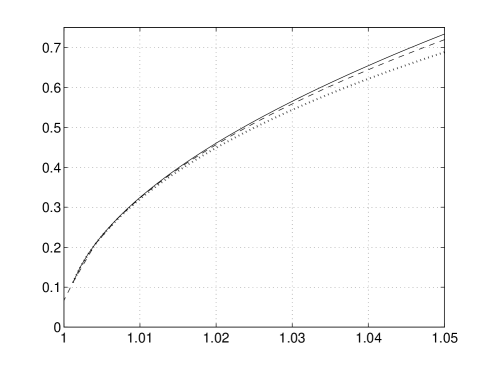
Figure 1: The conformal distance $\tau_{\hbox{\scriptsize sls}}$ to the surface of last scattering is shown in dependence on $\Omega_{\hbox{\scriptsize tot}}$. The full curve is obtained by varying only $\Omega_{\Lambda}$ as it is the case in our simulations. Alternatively, the variation in $\Omega_{\hbox{\scriptsize tot}}$ is achieved by changing only $\Omega_{\hbox{\scriptsize mat}}$ in the dotted curve and by changing the Hubble parameter $h$ in the dashed curve.

The following statistical analysis is based on the same cosmological parameters as in [19] which are close to the standard concordance model of cosmology [40]. The parameters are taken from the LAMBDA website (lambda.gsfc.nasa.gov), where we select the WMAP cosmological parameters of the model ’olcdm+sz+lens’ using the data ’wmap7+bao+snconst’, which are $\Omega_{\hbox{\scriptsize b}}=0.0485$, $\Omega_{\hbox{\scriptsize cdm}}=0.238$, the Hubble constant $h=0.681$, and the spectral index $n_{\hbox{\scriptsize s}}=0.961$. The total density parameter $\Omega_{\hbox{\scriptsize tot}}$ is varied by altering the density parameter of the cosmological constant $\Omega_{\scriptsize\Lambda}$, so that the total density covers the interval $\Omega_{\hbox{\scriptsize tot}}=1.001,\dots,1.05$. This $\Omega_{\hbox{\scriptsize tot}}$ interval is a bit larger than the 99% CL interval of the constraint $0.99<\Omega_{\hbox{\scriptsize tot}}<1.02$ (95% CL) which belongs to the chosen set of cosmological parameters. Our analysis of polyhedral double-action manifolds covers more than 2.6 million simulations which are computed for the different values of $\Omega_{\hbox{\scriptsize tot}}$ up to $\Omega_{\hbox{\scriptsize tot}}=1.05$ and for different observer positions. This large number of simulations is the reason why we restrict our variation of $\Omega_{\hbox{\scriptsize tot}}$ to a variation in $\Omega_{\scriptsize\Lambda}$. There are other ways of varying $\Omega_{\hbox{\scriptsize tot}}$, but since the main effect on the CMB on large angular scales is due to the distance $\tau_{\hbox{\scriptsize sls}}$ to the surface of last scattering, it suffice to confine to one method of variation. In order to emphasise this fact, figure 1 shows $\tau_{\hbox{\scriptsize sls}}$ as a function of $\Omega_{\hbox{\scriptsize tot}}$ whereas the modification of $\Omega_{\hbox{\scriptsize tot}}$ is achieved in three different ways, i. e. by varying only $\Omega_{\scriptsize\Lambda}$ (full curve), by varying only $\Omega_{\hbox{\scriptsize mat}}$ (dotted curve) and by varying the Hubble parameter $h$ (dashed curve). As seen in figure 1, the three curves differ only for values of $\Omega_{\hbox{\scriptsize tot}}$ towards $\Omega_{\hbox{\scriptsize tot}}=1.05$. Thus, for the analysis of topological suppressions of correlations on large angles, the manner in which the change in $\Omega_{\hbox{\scriptsize tot}}=1.05$ is realized has only a minor influence on the following results.

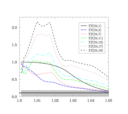
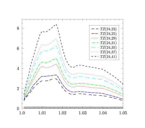
Figure 2: The minima $S_{\hbox{\scriptsize min}(\alpha,\rho)}$ of the $S$ statistics defined in eq. (14) are shown for all polyhedral double-action manifolds up to a group order of 1 000 as a function of the total density $\Omega_{\hbox{\scriptsize tot}}$. The horizontal thick line at 0.11 allows the comparison with the minima of the polyhedral spaces ${\cal T}\equiv TZ(24,1)$, ${\cal O}\equiv OZ(48,1)$, and ${\cal I}\equiv IZ(120,1)$ whose $\Omega_{\hbox{\scriptsize tot}}$-dependent values are shown as full black curves. The grey band indicates the range for the $S$ statistics obtained from the ILC seven year map with and without the KQ75 mask.

The figure 2 shows $S_{\hbox{\scriptsize min}(\alpha,\rho)}$ defined in eq. (14) where the minimum of the $S$ statistics is taken over all observer positions $(\alpha,\rho)$ possessing distinct CMB ensemble averages. The four panels show $S_{\hbox{\scriptsize min}(\alpha,\rho)}$ for all polyhedral double-action manifolds whose group order is below 1 000. In order to compare the model results with the observed ones, the correlation function $C^{\hbox{\scriptsize obs}}(\vartheta)$ is computed from the ILC 7 year map [41] which gives $S_{\hbox{\scriptsize ILC}}(60^{\circ})=8\,033\,\mu\hbox{K}^{4}$. By applying the KQ75 7yr mask [41] to the ILC 7 year map, a correlation function $C^{\hbox{\scriptsize obs}}(\vartheta)$ is obtained which leads to the even lower value $S_{\hbox{\scriptsize ILC,KQ75}}(60^{\circ})=1\,153\,\mu\hbox{K}^{4}$. Both values can be considered as an estimate of the boundaries of the uncertainty range, since the KQ75 7yr mask is the most conservative mask and applying no mask is the other extreme point of view. The application of the KQ75 7yr mask eliminates the pixels whose CMB fluctuations are obscured by foreground emissions mainly originating in the Galaxy. This range for the observed $S$ statistics in shown in figure 2 as the grey horizontal band where we have taken our normalisation into account. Note that the normalisation to the simply connected ${\cal S}^{3}$ space gives for the concordance model a value of one. This emphasises the discrepancy due to this correlation measure. The analysis of [4] shows that only 0.025 per cent of realisations of the concordance model possess such a low correlation.

The 13 double-action manifolds based on the binary tetrahedral space ${\cal T}$ are distributed over the panels (a) and (b) in ascending order. The correlation measure $S_{\hbox{\scriptsize min}(\alpha,\rho)}$ of the binary tetrahedral space ${\cal T}\equiv TZ(24,1)$ is shown in panel (a). Its first minimum occurs at $\Omega_{\hbox{\scriptsize tot}}\simeq 1.07$ and lies outside the displayed range $\Omega_{\hbox{\scriptsize tot}}\in[1.001,1.05]$. The minima of the three binary polyhedral spaces ${\cal T}$, ${\cal O}$, and ${\cal I}$ lie close together about $0.11$ which is indicated by the horizontal thick line. A significantly stronger suppression of CMB correlations than for ${\cal T}$ is revealed by the spaces $TZ(24,5)$ and $TZ(24,7)$. At the boundary of the 95% CL interval of $\Omega_{\hbox{\scriptsize tot}}=1.02$, the best candidate is the $TZ(24,5)$ space with $S_{\hbox{\scriptsize min}(\alpha,\rho)}\simeq 0.4$. The space $TZ(24,11)$ behaves approximately as ${\cal T}$. But for higher group orders $n$ of the cyclic group $Z_{n}$, a systematic increase of $S_{\hbox{\scriptsize min}(\alpha,\rho)}$ is observed, so that these models with larger values of $n$ do not provide viable models for the description of our Universe. The figure 2(b) shows this monotonic increase for the spaces obtained from $Z_{23}$ up to $Z_{41}$.

For the double-action manifolds derived from the binary octahedral space ${\cal O}$, there are more interesting space forms as revealed by figure 2(c). The octahedral double-action spaces $OZ(48,5)$ to $OZ(48,17)$ possess an even stronger suppression for most of the considered values of $\Omega_{\hbox{\scriptsize tot}}$ compared to ${\cal O}\equiv OZ(48,1)$. For the space ${\cal O}$ the strongest CMB suppression occurs close to $\Omega_{\hbox{\scriptsize tot}}=1.04$. Several octahedral double-action spaces possess values of $S_{\hbox{\scriptsize min}(\alpha,\rho)}$ that are even lower than the best value of $\sim 0.11$ of the three binary polyhedral spaces ${\cal T}$, ${\cal O}$, and ${\cal I}$, see the interval $\Omega_{\hbox{\scriptsize tot}}\in[1.03,1.04]$ in panel (c). As can be read off from the figure, the octahedral double-action manifolds $OZ(48,n)$, with $n=7$, 11, 13, 17, and 19 have suppression factors below 0.11. The space with $n=5$ obtains its minimum slightly above $\Omega_{\hbox{\scriptsize tot}}=1.04$. The table 2 lists the positions corresponding to the minima $S_{\hbox{\scriptsize min}(\Omega_{\hbox{\scriptsize tot}},\alpha,\rho)}$. Except for $OZ(48,19)$ the minima occur at nearly the same positions in the $\alpha$-$\rho$ plane. Furthermore, the correlation measure $S_{\hbox{\scriptsize min}(\alpha,\rho)}$ of the space $OZ(48,19)$ displays a similar behaviour as those of ${\cal O}$ for smaller values of $\Omega_{\hbox{\scriptsize tot}}$. In contrast to the tetrahedral double-action manifolds $TZ(24,n)$, there is no simple behaviour with respect to the increase of $S_{\hbox{\scriptsize min}(\alpha,\rho)}$ in terms of $n$ for the class $OZ(48,n)$ for $n\leq 19$. For $\Omega_{\hbox{\scriptsize tot}}\leq 1.02$, the best candidate is $OZ(48,5)$ with $S_{\hbox{\scriptsize min}(\alpha,\rho)}\simeq 0.2$. The spaces with $n=7$, 11, and 13 have also a pronounced suppression of $S_{\hbox{\scriptsize min}(\alpha,\rho)}\simeq 0.30$, 0.31, and 0.38, respectively, at $\Omega_{\hbox{\scriptsize tot}}=1.02$.

manifold ${\cal M}$	$S_{\hbox{\scriptsize min}(\Omega_{\hbox{\scriptsize tot}},\alpha,\rho)}$	$\Omega_{\hbox{\scriptsize tot}}$	$\rho$	$\alpha$
$OZ(48,5)$	0.080	1.044	0.141	0.785
$OZ(48,7)$	0.048	1.036	0.134	0.785
$OZ(48,11)$	0.032	1.038	0.141	0.785
$OZ(48,13)$	0.030	1.038	0.141	0.785
$OZ(48,17)$	0.035	1.040	0.157	0.785
$OZ(48,19)$	0.040	1.040	0.778	0.481
$IZ(120,7)$	0.075	1.021	0.126	0.628

Table 2: The parameters $\Omega_{\hbox{\scriptsize tot}},\rho,\alpha$ for which $S_{\hbox{\scriptsize min}(\Omega_{\hbox{\scriptsize tot}},\alpha,\rho)}$ reveals a local minimum are listed for the 6 double action manifolds $OZ(24,n)$, $n=5$, 7, 11, 13, 17, and 19 and for the double action manifold $IZ(120,7)$.

There exists only one icosahedral double-action space $IZ(120,n)$ whose group order is below 1 000, and that is the space $IZ(120,7)$. Its behaviour is compared to the binary icosahedral space ${\cal I}\equiv IZ(120,1)$ in figure 2(d). It is seen that the suppression is more pronounced for $IZ(120,7)$ than for ${\cal I}$. As it was the case for some octahedral double-action spaces, there is again a density range $\Omega_{\hbox{\scriptsize tot}}$ with a suppression stronger than $\sim 0.11$. The table 2 gives the position of the minimum at $\Omega_{\hbox{\scriptsize tot}}=1.021$ which is slightly larger than the values close to $\Omega_{\hbox{\scriptsize tot}}=1.05$. The first minimum of $S_{\hbox{\scriptsize min}(\alpha,\rho)}$ at $\Omega_{\hbox{\scriptsize tot}}=1.007$ has the remarkable suppression of $S_{\hbox{\scriptsize min}(\alpha,\rho)}=0.27$ which is smaller than the best values of all investigated spherical manifolds for $\Omega_{\hbox{\scriptsize tot}}\leq 1.01$.

Therefore, among the polyhedral double-action spaces are examples for multiconnected spaces that display a large suppression of CMB correlations for angle separations larger than $\vartheta\geq 60^{\circ}$.

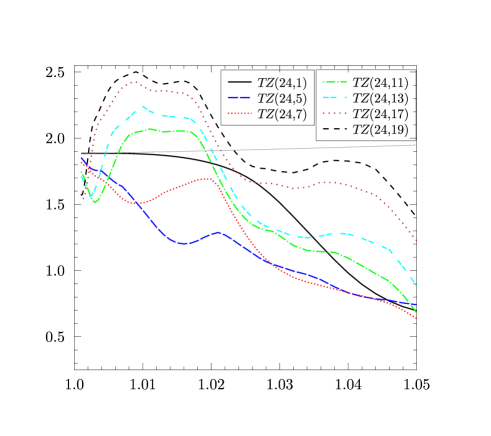
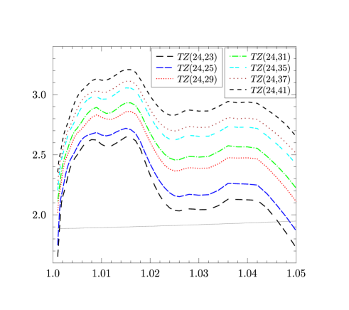
Figure 3: The minima $I_{\hbox{\scriptsize min}(\alpha,\rho)}(\Omega_{\hbox{\scriptsize tot}})$, defined in eq. (16), are shown for the tetrahedral double-action manifolds $TZ(24,n)$ in panels (a) and (b), the octahedral double-action manifolds $OZ(48,n)$ in panel (c), and for the icosahedral double-action manifold $IZ(120,7)$ in panel (d). The double-action correlation functions are compared to the observed correlation function $C^{\hbox{\scriptsize obs}}(\vartheta)$ obtained from the WMAP 7 year ILC map without applying any mask. The full grey curve shows $I(\Omega_{\hbox{\scriptsize tot}})$ for the spherical 3-space ${\cal S}^{3}$, i. e. for the simply connected space.

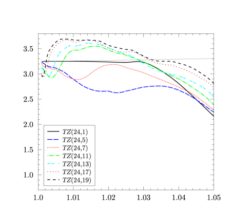
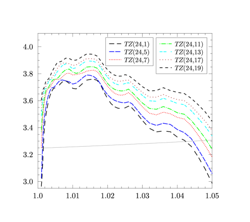
Figure 4: This figure also shows $I_{\hbox{\scriptsize min}(\alpha,\rho)}(\Omega_{\hbox{\scriptsize tot}})$ as in figure 3, but now the observed correlation function $C^{\hbox{\scriptsize obs}}(\vartheta)$ is obtained from the WMAP 7 year ILC map by applying the KQ75 mask.

While we have just discussed the correlation measure $S$, which provides a direct description of the large-angle behaviour of the multiconnected spaces, we now turn to the integrated weighted temperature correlation difference $I$, defined in eq. (15). It reveals how well the ensemble averages of the correlation functions $C(\vartheta)$ of the double-action spaces match $C^{\hbox{\scriptsize obs}}(\vartheta)$, which derives from the observed single realisation of the CMB sky admissible to us. The ILC seven year map is used for the computation of the observed correlation function $C^{\hbox{\scriptsize obs}}(\vartheta)$. In order to provide an impression of the experimental accuracy, the analysis is carried out with the full ILC map as well as with the ILC map subjected to the KQ75 seven year mask. As discussed above, the differences between these two analyses reflect the accuracy of the data. An alternative choice would be to use the $C^{\hbox{\scriptsize obs}}(\vartheta)$ obtained from the W or V band maps, but it is shown in [4] that the correlation functions are very similar to those belonging to the ILC map after applying the KQ75 seven year mask. Since no significantly changed result is expected, we restrict us in the following to the ILC map.

The minima $I_{\hbox{\scriptsize min}(\alpha,\rho)}(\Omega_{\hbox{\scriptsize tot}})$ are shown for all polyhedral double-action spaces up to the group order 1 000 in figures 3 and 4 as a function of $\Omega_{\hbox{\scriptsize tot}}$. The curves belonging to the multiconnected spaces should be compared to the simply connected case, i. e. the spherical 3-space ${\cal S}^{3}$, which is shown as the almost horizontal grey curve in figures 3 and 4. The double-action correlations describe the observed data better than those of the simply connected space if they lie below the full grey curve.

The tetrahedral double-action manifolds $TZ(24,n)$ are displayed in panels (a) and (b) of the figures 3 and 4. The general trend for the increasing strength of the correlations with increasing group order $n$ of the cyclic group $Z_{n}$, which was already discovered in the analysis of the $S$ statistics, is also reflected in the behaviour of $I_{\hbox{\scriptsize min}(\alpha,\rho)}(\Omega_{\hbox{\scriptsize tot}})$. The spaces $TZ(24,5)$ and $TZ(24,7)$ give a better match to the observed data than the binary tetrahedral space ${\cal T}$ which in turn describes the data better than the simply connected space. Except for values of $\Omega_{\hbox{\scriptsize tot}}$ very close to one, the models with $n>20$ do not present interesting alternatives. Note that the quality of the match to the data deteriorates systematically with increasing values of $n$. Because of these large values of $I_{\hbox{\scriptsize min}(\alpha,\rho)}(\Omega_{\hbox{\scriptsize tot}})$, the panels 3(b) and 4(b) use a different scaling compared to panels (a), (c), and (d).

The systematic behaviour shown in panels 3(b) and 4(b) is not repeated in the case of the octahedral double-action manifolds $OZ(48,n)$ which are displayed in panel (c). For $\Omega_{\hbox{\scriptsize tot}}$ below $\Omega_{\hbox{\scriptsize tot}}\simeq 1.025$ there is a sequence of $OZ(48,n)$ spaces which provides the best description of the data. With decreasing value of $\Omega_{\hbox{\scriptsize tot}}$, these are the spaces with $n=5$, $7$, and $11$, see panels 3(c) and 4(c). For values of $\Omega_{\hbox{\scriptsize tot}}$ larger than $1.025$, however, one finds in the case without a mask four spaces with smaller values of $I_{\hbox{\scriptsize min}(\alpha,\rho)}(\Omega_{\hbox{\scriptsize tot}})$ which even beats the minimum of the binary octahedral space ${\cal O}$. These are the spaces $OZ(48,13)$, $OZ(48,11)$, $OZ(48,17)$, and $OZ(48,19)$. Applying the KQ75 mask to the ILC data, also the curve belonging to the $OZ(48,7)$ space drops below that of the binary octahedral space ${\cal O}$.

The icosahedral double-action manifold $IZ(120,7)$ does not lead to a better agreement with the data than the binary icosahedral space ${\cal I}$ at that value of $\Omega_{\hbox{\scriptsize tot}}$ where the latter space has its minimum in $I_{\hbox{\scriptsize min}(\alpha,\rho)}(\Omega_{\hbox{\scriptsize tot}})$. But for smaller values of $\Omega_{\hbox{\scriptsize tot}}$, the space $IZ(120,7)$ describes the data better than ${\cal I}$ as can be seen in figures 3(d) and 4(d).

The figures 3 and 4 bring out the quality of the description of the data with respect to the data of the full ILC map as well as to the data restricted by the KQ75 mask. The comparison between figure 3 and figure 4 reveals that the polyhedral double-action manifolds give a better match to the correlation function $C^{\hbox{\scriptsize obs}}(\vartheta)$ derived from the full ILC map. Furthermore, the positions of the minima of $I_{\hbox{\scriptsize min}(\alpha,\rho)}(\Omega_{\hbox{\scriptsize tot}})$ are shifted to larger values of $\Omega_{\hbox{\scriptsize tot}}$ when the KQ75 mask is applied. This behaviour is, for example, visible in the panels 3(d) and 4(d) where the binary icosahedral space ${\cal I}$ possesses a minimum at $\Omega_{\hbox{\scriptsize tot}}\simeq 1.016$ without mask and at $\Omega_{\hbox{\scriptsize tot}}\simeq 1.021$ with KQ75 mask. This demonstrates that the choice of the available data leads to a range of variation so that only general properties of the double-action manifolds can be inferred from figures 3 and 4.

manifold ${\cal M}$	$I_{\hbox{\scriptsize min}(\Omega_{\hbox{\scriptsize tot}},\alpha,\rho)}^{\hbox{\scriptsize no mask}}$	$\Omega_{\hbox{\scriptsize tot}}$	$I_{\hbox{\scriptsize min}(\Omega_{\hbox{\scriptsize tot}},\alpha,\rho)}^{\hbox{\scriptsize KQ75 mask}}$	$\Omega_{\hbox{\scriptsize tot}}$
${\cal S}^{3}$	1.885	1.001	3.249	1.001
$OZ(48,5)$	0.744	1.017	2.159	1.020
$OZ(48,7)$	1.086	1.014	2.383	1.020
$OZ(48,11)$	1.085	1.020	2.421	1.020
$OZ(48,13)$	1.112	1.020	2.491	1.020
$OZ(48,17)$	1.187	1.020	2.523	1.020
$OZ(48,19)$	1.313	1.020	2.601	1.020
$IZ(120,7)$	0.999	1.015	1.667	1.020

Table 3: The table lists the manifolds with the best agreement with the observed correlation function $C^{\hbox{\scriptsize obs}}(\vartheta)$ which is obtained either from the full ILC map (no mask, columns 2 and 3) or after applying the KQ75 mask (columns 4 and 5). The interval of $\Omega_{\hbox{\scriptsize tot}}$ is restricted to $\Omega_{\hbox{\scriptsize tot}}\leq 1.02$. The value of ${\cal S}^{3}$, which corresponds to the concordance model, is also given.

Summarising, table 3 gives the promising models, which have below $\Omega_{\hbox{\scriptsize tot}}=1.02$ the most pronounced minima in the $I$ statistics. The columns 2 and 3 refer to the analysis without a mask which is shown in figure 3, whereas columns 4 and 5 gives the values for the KQ75 mask case shown in figure 4. With the restriction $\Omega_{\hbox{\scriptsize tot}}\leq 1.02$, the best model is given by $OZ(48,5)$ at $\Omega_{\hbox{\scriptsize tot}}=1.017$, if the full ILC map is used. The next best space is provided by $IZ(120,7)$ at $\Omega_{\hbox{\scriptsize tot}}=1.015$. Their values of $I_{\hbox{\scriptsize min}(\Omega_{\hbox{\scriptsize tot}},\alpha,\rho)}^{\hbox{\scriptsize no mask}}$ are significantly lower than the value $1.885$ belonging to the concordance model. Table 3 reveals that the application of the KQ75 mask leads to minimal values for the $I$ statistics at the interval boundary $\Omega_{\hbox{\scriptsize tot}}=1.02$. The best model is now $IZ(120,7)$ followed by the octahedral double-action manifolds $OZ(48,n)$ whose ranking with respect to the $I$ statistics is identical to the sequence of $n$, i. e. they are ranked by their volume.

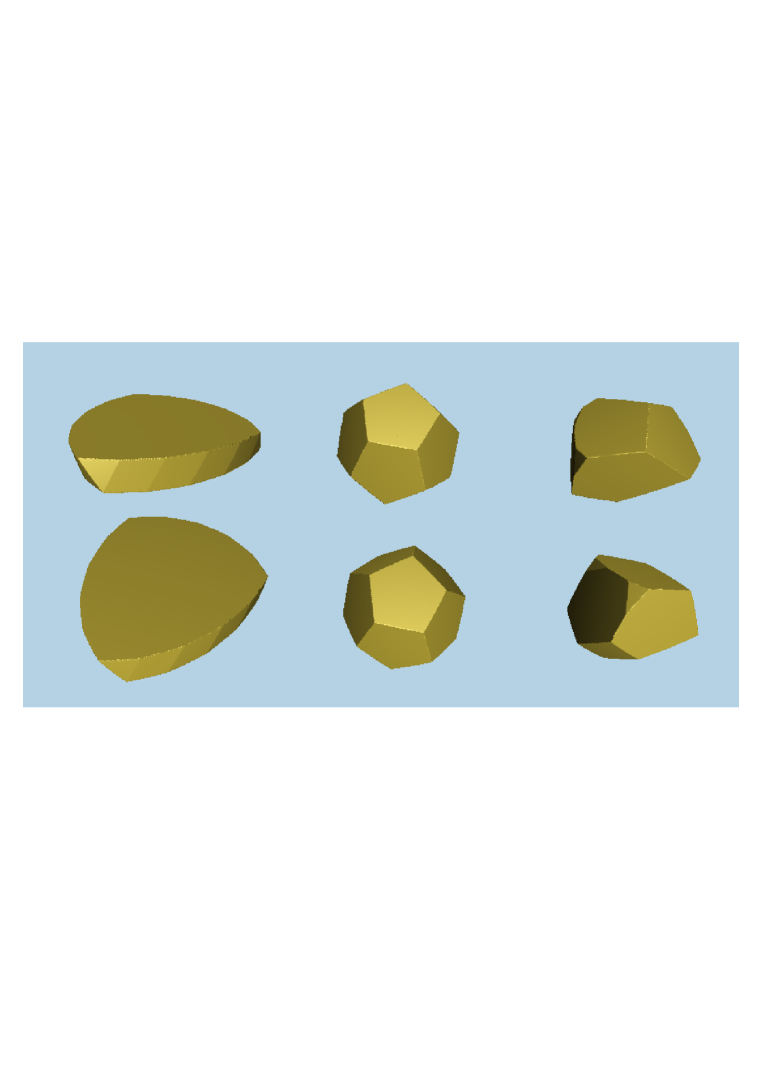
Figure 5: The Dirichlet domain of the tetrahedral double-action manifold $TZ(24,5)$ is shown as seen from three different observer positions. Two different projections are depicted for each observer position. At left the observer is at $\rho=0$ and $\alpha=0$, in the middle column the position is chosen to be at $\rho=0.691$ and $\alpha=0.659$ which corresponds to the shape of the dodecahedron. The right column shows the Dirichlet domain where the first minimum occurs in $S_{\hbox{\scriptsize min}(\alpha,\rho)}$ at $\Omega_{\hbox{\scriptsize tot}}\simeq 1.15$.

In [19] we pointed out that the two prism double-action manifolds $DZ(8,3)$ and $DZ(16,3)$ possess for a special observer position a Dirichlet domain identical to the binary tetrahedral space ${\cal T}$ and to the binary octahedral space ${\cal O}$, respectively. The Dirichlet domain of the binary icosahedral space ${\cal I}$ does not emerge among the class of prism double-action manifolds. This Dirichlet domain, however, is obtained from the tetrahedral double-action manifold $TZ(24,5)$ again for a special observer position. In figure 5 the Dirichlet domains of $TZ(24,5)$ are shown for three observer positions. At $\rho=0.691$ and $\alpha=0.659$ the dodecahedron emerges which is also the Dirichlet domain of the binary icosahedral space ${\cal I}$. Thus, the special Dirichlet domains of all three binary polyhedral spaces can be found within the class of the double-action manifolds. Also shown is the Dirichlet domain for that observer position where the largest suppression of CMB correlations on large scales occurs as measured by $S_{\hbox{\scriptsize min}(\alpha,\rho)}$. This minimum, which is obtained at $\Omega_{\hbox{\scriptsize tot}}\simeq 1.15$, corresponds to the Dirichlet domain shown at the right hand side of figure 5. Remarkably, it is not the most regular Dirichlet domain which thus demonstrates that oddly shaped domains can lead to a stronger CMB suppression than well-proportioned ones.

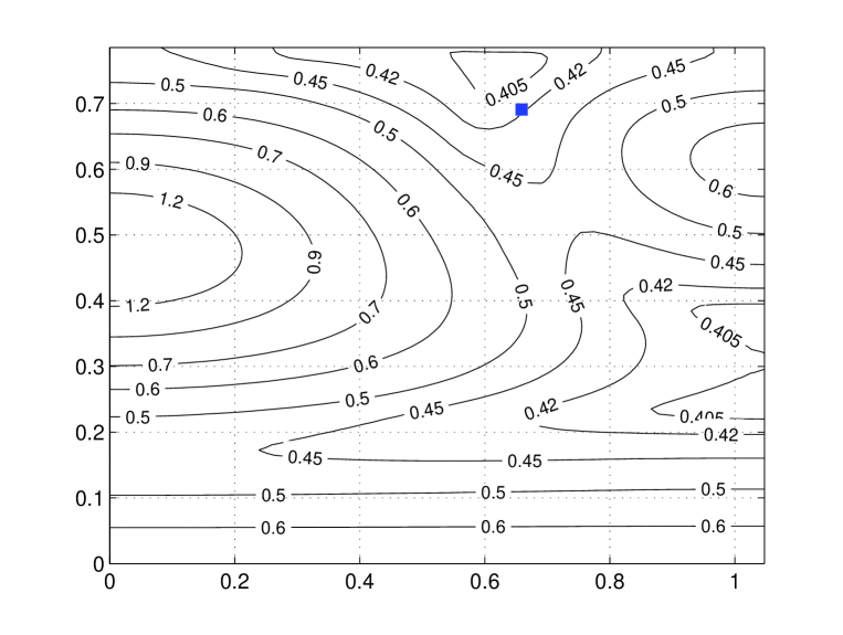
Figure 6: The $\alpha$-$\rho$ dependence of the $S$ statistics is displayed for the manifold $TZ(24,5)$ at $\Omega_{\hbox{\scriptsize tot}}=1.02$ normalised by the value $S_{{\cal S}^{3}}$ of the simply connected space. The full square indicates the position $\rho=0.691$ and $\alpha=0.659$ where the Dirichlet domain of the space $TZ(24,5)$ has the shape of the dodecahedron.

This point is emphasised by figure 6 where the correlation measure $S$ is plotted for $\Omega_{\hbox{\scriptsize tot}}=1.02$ in such a way that the full observer dependence can be inferred. The value of $\Omega_{\hbox{\scriptsize tot}}=1.02$ is selected because at that value the binary icosahedral space ${\cal I}$ provides the best description of the CMB correlations. The figure reveals a region in the $\alpha$-$\rho$ plane where the correlation measure $S$ yields values larger than those of the simply connected ${\cal S}^{3}$ space. But besides this region around $\alpha=0$ and $\rho=0.5$, the values of $S$ drop to values as low as $0.4$. The minimal values are obtained for three positions at $(\alpha,\rho)\simeq(0.63,0.74)$, $(\alpha,\rho)\simeq(\pi/3,0.24)$, and $(\alpha,\rho)\simeq(\pi/3,0.38)$. Although the position $\alpha=0.659$ and $\rho=0.691$ with the dodecahedral Dirichlet domain is not very far from one of the three minima, it is nevertheless not the position giving the minimum.

4 Summary and Discussion

This paper analyses the large-scale correlations in the CMB sky for the polyhedral double-action manifolds. With this analysis, the CMB correlations are finally investigated for all double-action manifolds since those belonging to the lens spaces and to the prism double-action manifolds are already studied in [18] and [19]. The large-scale correlation measure (14) is used in order the search for spaces with a significant suppression of correlations in the CMB anisotropy on scales above $\vartheta>60^{\circ}$. This quantity is normalised to the simply connected spherical space ${\cal S}^{3}$. The lens spaces $L(p,q)$ can lead to a suppression relative to ${\cal S}^{3}$ by a factor of about $\sim 0.5$ [18]. The lens spaces with such a large suppression have lenticular fundamental cells whose two faces have to be rotated by a relative angle of $\sim 101^{\circ}$ or $\sim 137^{\circ}$ before the faces are identified. Among the prism double-action manifolds $DZ(p,n)$, there are spaces with even smaller large-scale correlations with suppression factors in the range $0.3\dots 0.4$. The three best candidates are $DZ(8,3)$, $DZ(16,3)$, and $DZ(20,3)$ [19]. Although this CMB suppression is remarkable, it is less pronounced than in the cases of the three binary polyhedral spaces ${\cal T}$, ${\cal O}$, and ${\cal I}$ where the suppression factor is of the order of $0.11$.

The three binary polyhedral spaces ${\cal T}$, ${\cal O}$, and ${\cal I}$ lead to the three classes $TZ(24,n)$, $OZ(48,n)$, and $IZ(120,n)$ of polyhedral double-action manifolds. The analysis of this paper shows that several polyhedral double-action manifolds can possess even stronger suppressions than those found in the three binary polyhedral spaces (see figure 2). From these spaces, the octahedral double-action manifolds $OZ(48,n)$ with $n=7$, 11, 13, 17, and 19 have suppression factors below 0.11 for $\Omega_{\hbox{\scriptsize tot}}$ in the range $\Omega_{\hbox{\scriptsize tot}}=1.03\dots 1.04$. With the constraint $\Omega_{\hbox{\scriptsize tot}}\leq 1.02$, the best octahedral double-action manifold is the space $OZ(48,5)$ with a suppression factor 0.2. In addition, three further octahedral spaces with $n=7$, 11, and 13 possess suppression factors between 0.3 and 0.4 in that $\Omega_{\hbox{\scriptsize tot}}$ range.

The icosahedral double-action manifold $IZ(120,7)$ also reveals an interesting behaviour with a suppression factor below 0.11 close to $\Omega_{\hbox{\scriptsize tot}}=1.02$. Remarkably, insisting on the constraint $\Omega_{\hbox{\scriptsize tot}}\leq 1.01$, the space $IZ(120,7)$ has the largest suppression of all investigated spherical manifolds. The minimum in the correlation measure is obtained at $\Omega_{\hbox{\scriptsize tot}}=1.007$ with a suppression factor of 0.27.

The tetrahedral double-action manifolds $TZ(24,n)$ do not provide comparable candidates to explain the low correlations on the CMB sky at large angles. They possess such small suppression factors only for significantly larger values of the total density $\Omega_{\hbox{\scriptsize tot}}$ which are beyond the range considered in this paper. Some $TZ(24,n)$ spaces have nevertheless CMB suppressions comparable to the prism double-action manifolds $DZ(p,n)$ mentioned above.

The ensemble averages of the correlation functions $C(\vartheta)$ of the polyhedral double-action manifolds are also compared to the observed $C^{\hbox{\scriptsize obs}}(\vartheta)$ using the $I$ statistics. This analysis confirms the result obtained from the $S$ statistics.

Concluding, there are five octahedral double-action manifolds and one icosahedral double-action manifold with a group order below 1 000 with a pronounced suppression of CMB correlation on large angular scales which deserve further investigations.

Appendix A Matrix Representations of $\hbox{SU}(2,\mathbb{C})$

Every matrix $u\in\hbox{SU}(2,\mathbb{C})$ can be written as

$$u\;=\;{\bf 1}w+\hbox{i}\,\sigma_{x}x+\hbox{i}\,\sigma_{y}y+\hbox{i}\,\sigma_{z}z\;=\;\left(\begin{array}[]{cc}w+\hbox{i}\,z&\hbox{i}\,\left(x-\hbox{i}\,y\right)\\ \hbox{i}\,\left(x+\hbox{i}\,y\right)&w-\hbox{i}\,z\end{array}\right)\hskip 10.0pt$$ (17)

with the restriction $w^{2}+x^{2}+y^{2}+z^{2}=1$. Here the Pauli matrices are denoted by

$$\sigma_{x}\;=\;\left(\begin{array}[]{cc}0&1\\ 1&0\end{array}\right)\hskip 10.0pt,\hskip 10.0pt\sigma_{y}\;=\;\left(\begin{array}[]{cc}0&-\hbox{i}\\ \hbox{i}&0\end{array}\right)\hskip 10.0pt,\hskip 10.0pt\hbox{and}\hskip 10.0pt\sigma_{z}\;=\;\left(\begin{array}[]{cc}1&0\\ 0&-1\end{array}\right)$$

and ${\bf 1}$ is the identity matrix. Since $\hbox{SU}(2,\mathbb{C})$ can be identified with the 3-sphere ${\cal S}^{3}$, the matrix $u$ can be interpreted as a coordinate matrix which describes points on the 3-sphere ${\cal S}^{3}$ with the Cartesian coordinates $(w,x,y,z)$. An alternative choice of coordinates $(\rho,\alpha,\epsilon)$ on ${\cal S}^{3}$ is related to these Cartesian coordinates $(w,x,y,z)$ by

$$\left(\begin{array}[]{c}w\\ x\\ y\\ z\end{array}\right)=\left(\begin{array}[]{c}\cos\rho\cos\alpha\\ \sin\rho\sin\epsilon\\ \sin\rho\cos\epsilon\\ \cos\rho\sin\alpha\end{array}\right)\hskip 10.0pt$$

with $\rho\in[0,\pi/2]$, $\alpha,\epsilon\in[0,2\pi]$. In terms of the coordinates $(\rho,\alpha,\epsilon)$, the matrix $u$ reads

$$u(\rho,\alpha,\epsilon)\;=\;\left(\begin{array}[]{cc}\cos\rho\,e^{+\hbox{\scriptsize i}\alpha}&\sin\rho\,e^{+\hbox{\scriptsize i}\epsilon}\\ -\sin\rho\,e^{-\hbox{\scriptsize i}\epsilon}&\cos\rho\,e^{-\hbox{\scriptsize i}\alpha}\end{array}\right)\hskip 10.0pt.$$ (18)

This parametrisation of a $\hbox{SU}(2,\mathbb{C})$ matrix is used for the transformation $t$ in section 2, see eq. (7). It facilitates computations involving the Wigner polynomials since the matrix elements of $u(\rho,\alpha,\epsilon)$ are given by $D^{1/2}_{\pm 1/2,\pm 1/2}(u)$.

However, for the analysis involving the spherical coordinates $(\tau,\theta,\phi$), it is more convenient to use

$$\left(\begin{array}[]{c}w\\ x\\ y\\ z\end{array}\right)=\left(\begin{array}[]{c}\cos\tau\\ \sin\tau\sin\theta\cos\phi\\ \sin\tau\sin\theta\sin\phi\\ \sin\tau\cos\theta\end{array}\right)\hskip 10.0pt$$

with $\tau,\theta\in[0,\pi]$, $\phi\in[0,2\pi]$. Then, the matrix $u=u(\tau,\theta,\phi)$ reads

$$u(\tau,\theta,\phi)\;=\;\left(\begin{array}[]{cc}\cos\tau+\hbox{i}\,\sin\tau\cos\theta&\hbox{i}\,\sin\tau\sin\theta\,\rme^{-\hbox{\scriptsize i}\phi}\\ \hbox{i}\,\sin\tau\sin\theta\,\rme^{\hbox{\scriptsize i}\phi}&\cos\tau-\hbox{i}\,\sin\tau\cos\theta\end{array}\right)\hskip 10.0pt.$$ (19)

The origin of the coordinate system $(w,x,y,z)=(1,0,0,0)\equiv{\bf 1}$ can be shifted to the point $u(\tau,\theta,\phi)$ using the transformation $g(\tau,\theta,\phi):{\bf 1}\rightarrow u(\tau,\theta,\phi)=g_{a}^{-1}(\tau,\theta,\phi)\,{\bf 1}\,g_{b}(\tau,\theta,\phi)$, where

$$g(\tau,\theta,\phi)\;=\;\left(g_{a}(\tau,\theta,\phi),g_{b}(\tau,\theta,\phi)\right)$$ (20)

with

$$g_{a}(\tau,\theta,\phi)\;=\;\left(\begin{array}[]{cc}e^{-\hbox{\scriptsize i}\frac{\tau}{2}}&0\\ 0&e^{\hbox{\scriptsize i}\frac{\tau}{2}}\end{array}\right)\left(\begin{array}[]{cc}\sin\frac{\theta}{2}&\cos\frac{\theta}{2}\\ -\cos\frac{\theta}{2}&\sin\frac{\theta}{2}\end{array}\right)\left(\begin{array}[]{cc}e^{\hbox{\scriptsize i}\frac{\phi}{2}}&0\\ 0&e^{-\hbox{\scriptsize i}\frac{\phi}{2}}\end{array}\right)$$

and

$$g_{b}(\tau,\theta,\phi)\;=\;\left(\begin{array}[]{cc}e^{\hbox{\scriptsize i}\frac{\tau}{2}}&0\\ 0&e^{-\hbox{\scriptsize i}\frac{\tau}{2}}\end{array}\right)\left(\begin{array}[]{cc}\sin\frac{\theta}{2}&\cos\frac{\theta}{2}\\ -\cos\frac{\theta}{2}&\sin\frac{\theta}{2}\end{array}\right)\left(\begin{array}[]{cc}e^{\hbox{\scriptsize i}\frac{\phi}{2}}&0\\ 0&e^{-\hbox{\scriptsize i}\frac{\phi}{2}}\end{array}\right)\hskip 10.0pt.$$

Appendix B Eigenmodes on the 3-Sphere in the Spherical Coordinates

The aim of this section is to derive the factorisation of the eigenmodes of the Laplace-Beltrami operator in terms of the usual spherical harmonics $Y_{lm}(\theta,\phi)$ and a radial function, and furthermore, to find a Fourier expansion for the radial function [23], which simplifies the numerical computation of the eigenmodes of multiconnected spaces.

The eigenmodes are given in spherical coordinates as

$$\Psi_{jlm}(\tau,\theta,\phi):=\langle\tau,\theta,\phi|j;l,m\rangle=\langle 0,0,0|D(\tau,\theta,\phi)|j;l,m\rangle\hskip 10.0pt$$ (21)

with $D(\tau,\theta,\phi)=e^{\hbox{\scriptsize i}\tau\left(-J_{az}+J_{bz}\right)}\,e^{\hbox{\scriptsize i}\theta(J_{ay}+J_{by})}\,e^{\hbox{\scriptsize i}\phi\left(J_{az}+J_{bz}\right)}$. In spherical coordinates, $D(\tau,\theta,\phi)$ shifts the origin $(0,0,0)$ to the point $(\tau,\theta,\phi)$, where the matrix representation of this transformation is given by eq. (20). Using the completeness relation $\sum_{l^{\prime}m^{\prime}}|j;l^{\prime},m^{\prime}\rangle\langle j;l^{\prime},m^{\prime}|={\bf 1}$, one can rewrite

$$\Psi_{jlm}(\tau,\theta,\phi)\;=\;\sum_{l^{\prime}m^{\prime}}\Psi_{jl^{\prime}m^{\prime}}(0,0,0)\,\langle j;l^{\prime},m^{\prime}|D(\tau,\theta,\phi)|j;l,m\rangle\hskip 10.0pt,$$

where $\Psi_{jl^{\prime}m^{\prime}}(0,0,0)=\langle 0,0,0|j;l^{\prime},m^{\prime}\rangle$. Because of the factorisation $\Psi_{jlm}(\tau,\theta,\phi)\sim R_{\beta}^{\,l}(\tau)Y_{lm}(\theta,\phi)$ with $\beta=2j+1$, $l=0,\dots,\beta-1$, one gets the property $\Psi_{jlm}(0,0,0)\sim\delta_{l,0}\delta_{m,0}$ from the spherical harmonics $Y_{lm}(\theta,\phi)$ and from $R_{\beta}^{\,l}(\tau)$ as defined in Eq. (A.21) in [42]. This simplifies (B) to

$$\Psi_{jlm}(\tau,\theta,\phi)\;=\;\Psi_{j00}(0,0,0)\,\langle j;0,0|D(\tau,\theta,\phi)|j;l,m\rangle\hskip 10.0pt.$$

With the help of the completeness relation $\sum_{m^{\prime}_{a}m^{\prime}_{b}}|j;m^{\prime}_{a},m^{\prime}_{b}\rangle\langle j;m^{\prime}_{a},m^{\prime}_{b}|={\bf 1}$ and the eigenvalue equation $\langle j;m^{\prime}_{a},m^{\prime}_{b}|e^{\hbox{\scriptsize i}\tau\left(-J_{az}+J_{bz}\right)}=\langle j;m^{\prime}_{a},m^{\prime}_{b}|e^{\hbox{\scriptsize i}\tau\left(-m^{\prime}_{a}+m^{\prime}_{b}\right)}$, the matrix element is manipulated

$$\langle j;l^{\prime},m^{\prime}|D(\tau,\theta,\phi)|j;l,m\rangle$$

$$= \sum_{m^{\prime}_{a}m^{\prime}_{b}}\langle j;l^{\prime},m^{\prime}|j;m^{\prime}_{a},m^{\prime}_{b}\rangle\langle j;m^{\prime}_{a},m^{\prime}_{b}|D(\tau,\theta,\phi)|j;l,m\rangle$$

$$= \sum_{m^{\prime}_{a}m^{\prime}_{b}}e^{\hbox{\scriptsize i}\tau\left(-m^{\prime}_{a}+m^{\prime}_{b}\right)}\langle j;l^{\prime},m^{\prime}|j;m^{\prime}_{a},m^{\prime}_{b}\rangle\langle j;m^{\prime}_{a},m^{\prime}_{b}|D(0,\theta,\phi)|j;l,m\rangle$$

$$= \sum_{m^{\prime}_{a}m^{\prime}_{b}m^{\prime\prime}_{a}m^{\prime\prime}_{b}}e^{\hbox{\scriptsize i}\tau\left(-m^{\prime}_{a}+m^{\prime}_{b}\right)}\langle j;m^{\prime}_{a},m^{\prime}_{b}|D(0,\theta,\phi)|j;m^{\prime\prime}_{a},m^{\prime\prime}_{b}\rangle$$

$$\hskip 100.0pt\times\;\langle j;l^{\prime},m^{\prime}|j;m^{\prime}_{a},m^{\prime}_{b}\rangle\,\langle j;m^{\prime\prime}_{a},m^{\prime\prime}_{b}|j;l,m\rangle\hskip 10.0pt.$$

Because of the product relation (3), one gets

$$\langle j;m^{\prime}_{a},m^{\prime}_{b}|D(0,\theta,\phi)|j;m^{\prime\prime}_{a},m^{\prime\prime}_{b}\rangle$$

$$= \langle jm^{\prime}_{a}|e^{\hbox{\scriptsize i}\theta J_{ay}}\,e^{\hbox{\scriptsize i}\phi J_{az}}|jm^{\prime\prime}_{a}\rangle\langle jm^{\prime}_{b}|e^{\hbox{\scriptsize i}\theta J_{by}}\,e^{\hbox{\scriptsize i}\phi J_{bz}}|jm^{\prime\prime}_{b}\rangle$$

$$= D^{\,j}_{m^{\prime}_{a},m^{\prime\prime}_{a}}(0,\theta,\phi)D^{\,j}_{m^{\prime}_{b},m^{\prime\prime}_{b}}(0,\theta,\phi)$$

$$= \sum_{l^{\prime\prime}}\langle j;m^{\prime}_{a},m^{\prime}_{b}|j;l^{\prime\prime},m^{\prime}\rangle\langle j;l^{\prime\prime},m^{\prime\prime}|j;m^{\prime\prime}_{a},m^{\prime\prime}_{b}\rangle D^{\,l^{\prime\prime}}_{m^{\prime},m^{\prime\prime}}(0,\theta,\phi)\hskip 10.0pt,$$

where the eq. (4.3.1) in [39] has been used. Here, the abbreviations $m^{\prime}:=m^{\prime}_{a}+m^{\prime}_{b}$ and $m^{\prime\prime}:=m^{\prime\prime}_{a}+m^{\prime\prime}_{b}$ have been introduced. Inserting this result into (B) leads with $\sum_{m^{\prime\prime}_{a}m^{\prime\prime}_{b}}\langle j;l^{\prime\prime},m^{\prime\prime}|j;m^{\prime\prime}_{a},m^{\prime\prime}_{b}\rangle\langle j;m^{\prime\prime}_{a},m^{\prime\prime}_{b}|j;l,m\rangle=\delta_{l^{\prime\prime},l}\delta_{m^{\prime\prime},m}$ to

$$\langle j;l^{\prime},m^{\prime}|D(\tau,\theta,\phi)|j;l,m\rangle$$

$$= \sum_{m^{\prime}_{a}m^{\prime}_{b}}e^{\hbox{\scriptsize i}\tau\left(-m^{\prime}_{a}+m^{\prime}_{b}\right)}\langle j;l^{\prime},m^{\prime}|j;m^{\prime}_{a},m^{\prime}_{b}\rangle\,\langle j;m^{\prime}_{a},m^{\prime}_{b}|j;l,m^{\prime}\rangle D^{\,l}_{m^{\prime},m}(0,\theta,\phi)\hskip 10.0pt.$$

Using the simplified matrix element (B), the eigenmode (B) is expressed as

$$\Psi_{jlm}(\tau,\theta,\phi) = \Psi_{j00}(0,0,0)\,D^{\,l}_{0,m}(0,\theta,\phi)$$

$$\times\sum_{m^{\prime}_{a}}e^{-\hbox{\scriptsize i}\tau 2m^{\prime}_{a}}\langle j;0,0|j;m^{\prime}_{a},-m^{\prime}_{a}\rangle\,\langle j;m^{\prime}_{a},-m^{\prime}_{a}|j;l,0\rangle\hskip 10.0pt.$$

With the relation $D^{\,l}_{0,m}(0,\theta,\phi)=\sqrt{\frac{4\pi}{2l+1}}Y_{lm}(\theta,\phi)$, Eq. (4.1.25) in [39], the normalisation of the eigenmode $\Psi_{jlm}(\tau,\theta,\phi)=\tilde{R}_{\beta}^{\,l}(\tau)Y_{lm}(\theta,\phi)$ to ${\cal S}^{3}$ leads to $\Psi_{j00}(0,0,0)=\sqrt{\frac{(2j+1)^{2}}{2\pi^{2}}}$ which is chosen to be real. Then the Fourier expansion of the radial function $\tilde{R}_{\beta}^{\,l}(\tau)$ can be read off as

$$\tilde{R}_{\beta}^{\,l}(\tau)\,=\,\sqrt{\frac{2\,(2j+1)^{2}}{\pi\,(2l+1)}}\sum_{m^{\prime}_{a}}\langle jm^{\prime}_{a}j-m^{\prime}_{a}|00\rangle\langle jm^{\prime}_{a}j-m^{\prime}_{a}|l0\rangle e^{-\hbox{\scriptsize i}2\,\tau m^{\prime}_{a}}\hskip 5.0pt,$$ (24)

where $\beta=2j+1$ and the notation of the Clebsch-Gordan coefficients have been introduced. The radial function $\tilde{R}_{\beta}^{\,l}(\tau)$ differs from $R_{\beta}^{\,l}(\tau)$ used in [42] by a phase factor according to $\tilde{R}_{\beta}^{\,l}(\tau)=(-\hbox{i})^{l}\,R_{\beta}^{\,l}(\tau)$.

Appendix C Eigenmodes on Binary Polyhedral Spaces

The eigenmodes of the binary polyhedral spaces are already investigated in [43, 44, 23]. These eigenmodes can also be computed as the special case $n=1$ of the ansatz (6), which incorporates the action of the generator of the cyclic group $Z_{n}$ and the action of the first generator (2) of the binary polyhedral groups $T^{\star}$, $O^{\star}$, or $I^{\star}$. These deck groups lead to the spaces ${\cal M}=TZ(24,1)$, $OZ(48,1)$, and $OZ(120,1)$.

At first, the ansatz (6) is expressed in terms of the spherical coordinates $(\tau,\theta,\phi)$. Using the completeness relation $\sum_{lm}|j;l,m\rangle\langle j;l,m|={\bf 1}$ one gets with eq. (21)

$$\psi^{\,\cal M}_{j;s,m_{b}}(\tau,\theta,\phi) := \langle\tau,\theta,\phi|j;s,m_{b}\rangle$$

$$= \sum_{m_{a}\equiv 0\;\hbox{\scriptsize mod}\;N}a^{s}_{m_{a}}\sum_{l}\langle jm_{a}jm_{b}|lm\rangle\Psi_{jlm}(\tau,\theta,\phi)\hskip 10.0pt$$

with $|m_{b}|\leq j$, $N=3$ (binary tetrahedral space), $N=4$ (binary octahedral space), or $N=5$ (binary icosahedral space). In the next step, the eigenmodes $\Psi_{jlm}(\tau,\theta,\phi)=\tilde{R}_{\beta}^{\,l}(\tau)Y_{lm}(\theta,\phi)$ are expressed by the Fourier expansion (24). To constrain the coefficients $a^{s}_{m_{a}}$, the invariance of the eigenmodes under the action of the second generator of the binary polyhedral group is taken into account by requiring $\psi^{\,\cal M}_{j;s,m_{b}}(\tau,\theta_{2},\phi_{2})-\psi^{\,\cal M}_{j;s,m_{b}}(\tau+\tau_{2},\theta_{2},\phi_{2})=0$, which leads to

$$\sum_{m_{a}\equiv 0\;\hbox{\scriptsize mod}\;N}a^{s}_{m_{a}}\sum_{lm^{\prime}_{a}}\langle jm_{a}jm_{b}|lm\rangle\sqrt{\frac{2\,(2j+1)^{2}}{\pi\,(2l+1)}}\langle jm^{\prime}_{a}j-m^{\prime}_{a}|00\rangle$$

$$\hskip 60.0pt\times\langle jm^{\prime}_{a}j-m^{\prime}_{a}|l0\rangle(1-e^{-\hbox{\scriptsize i}2\,\tau_{2}m^{\prime}_{a}})e^{-\hbox{\scriptsize i}2\,\tau m^{\prime}_{a}}Y_{lm}(\theta_{2},\phi_{2})=0\hskip 10.0pt.$$

This equation written as $\sum_{m_{a}^{\prime}}A_{m_{a}^{\prime}}e^{-\hbox{\scriptsize i}2\,\tau m^{\prime}_{a}}=0$ has to be valid for every value of $\tau$. Therefore, each coefficient $A_{m^{\prime}_{a}}$ with $m^{\prime}_{a}=-j,\dots,j$ has to vanish identically, and one gets $2j+1$ equations

$$\sum_{m_{a}\equiv 0\;\hbox{\scriptsize mod}\;N}a^{s}_{m_{a}}\sum_{l}\langle jm_{a}jm_{b}|lm\rangle\sqrt{\frac{2\,(2j+1)^{2}}{\pi\,(2l+1)}}\langle jm^{\prime}_{a}j-m^{\prime}_{a}|00\rangle$$ (25)

$$\hskip 60.0pt\times\langle jm^{\prime}_{a}j-m^{\prime}_{a}|l0\rangle(1-e^{-\hbox{\scriptsize i}2\,\tau_{2}m^{\prime}_{a}})Y_{lm}(\theta_{2},\phi_{2})=0\hskip 10.0pt.$$

The solution $a^{s}_{m_{a}}$ is independent of $m_{b}$, since the generators of the binary polyhedral group act only on $|j,m_{a}\rangle$, see ansatz (6). The set of equations for $a^{s}_{m_{a}}$ with $m_{a}=kN$ and $|m_{a}|\leq j$, $k\in\mathbb{Z}$ can be numerically solved using a singular value decomposition routine by choosing the value $m_{b}=0$ (see also (E.14) in [23]).

The eigenmodes of the binary polyhedral spaces are given in terms of the spherical basis $\Psi_{jlm}(\tau,\theta,\phi)$ by

$$\psi^{\,\cal M}_{j;i}(\tau,\theta,\phi)=\sum_{l=0}^{2j}\sum_{m=-l}^{l}\xi^{j,i}_{lm}({\cal M})\,\Psi_{jlm}(\tau,\theta,\phi)\;\;$$

$$\xi^{j,i}_{lm}({\cal M})=\langle jm_{a}jm_{b}(i)|lm\rangle a^{s(i)}_{m_{a}}$$ (26)

$$\hbox{with}\hskip 5.0ptm_{a}+m_{b}=m\hskip 5.0pt,\hskip 5.0ptm_{a}\equiv 0\;\hbox{mod}\;N\hskip 5.0pt\hbox{and}\hskip 5.0pt|m_{a}|,|m_{b}|\leq j\hskip 10.0pt,$$

where $i$ counts the degenerated modes. Since these manifolds are homogeneous, the eigenmodes can be chosen independent of the observer position. Note, that an additional phase factor $(-\hbox{i})^{l}$ has to be taken into account with respect to the radial function of [42].

Appendix D Eigenmodes on Polyhedral Double-Action Manifolds

In this section the eigenmodes of the Laplace-Beltrami operator on the polyhedral double-action manifolds ${\cal M}=TZ(24,n)$, $OZ(48,n)$, and $IZ(120,n)$, $n>1$, are derived in terms of the spherical basis (21). The action of the cyclic group $Z_{n}$ onto the ansatz (6) does not depend on the action of the polyhedral groups. Therefore, using the ansatz (6), the eigenmode for the observer position defined by the transformation $t$ is obtained

$$\hat{\psi}^{\,\cal M}_{j,i}(\tau,\theta,\phi) := D(t^{-1})\psi^{\,\cal M}_{j,i}(\tau,\theta,\phi)\;=\;\langle\tau,\theta,\phi|D(t^{-1})|j,i\rangle$$

$$= \sum_{m_{a}\equiv 0\;\hbox{\scriptsize mod}\;N}a^{s(i)}_{m_{a}}\;\langle\tau,\theta,\phi|D(t^{-1})|j;m_{a},m_{b}(i)\rangle$$

$$\hskip 80.0pt\hbox{with}\hskip 5.0pt2\,m_{b}\equiv 0\;\hbox{mod}\;n\hskip 10.0pt$$

in terms of the spherical coordinates $(\tau,\theta,\phi)$. Here, the solutions $a^{s}_{m_{a}}$ are determined by the set of equations (25). Because of the condition $2\,m_{b}\equiv 0\;\hbox{mod}\;n$, the manifolds with $n>1$ are inhomogeneous. For this reason an observer dependence has to be taken into account by the translation $D(t^{-1})=e^{\hbox{\scriptsize i}\,(-\alpha+\epsilon)\,J_{bz}}e^{\hbox{\scriptsize i}\,(-2\rho)\,J_{by}}e^{\hbox{\scriptsize i}\,(-\alpha-\epsilon)\,J_{bz}}$ which acts only on the states $|j,m_{b}\rangle$. Inserting the completeness relation $\sum_{lm}|j;l,m\rangle\langle j;l,m|={\bf 1}$, the eigenmodes can be rewritten in terms of the spherical basis $\Psi_{jlm}(\tau,\theta,\phi)$

$$\hat{\psi}^{\,\cal M}_{j,i}(\tau,\theta,\phi)=\sum_{lm}\sum_{m_{a}\equiv 0\;\hbox{\scriptsize mod}\;N}a^{s(i)}_{m_{a}}\;\langle j;l,m|D(t^{-1})|j;m_{a},m_{b}(i)\rangle\Psi_{jlm}(\tau,\theta,\phi)\hskip 1.0pt.$$ (27)

In the next step the completeness relation $\sum_{\tilde{m}_{b}}|j,\tilde{m}_{b}\rangle\langle j,\tilde{m}_{b}|={\bf 1}$ and eq. (2) are used to obtain the final expansion

$$\hat{\psi}^{\,\cal M}_{j;i}(\tau,\theta,\phi) = \sum_{l=0}^{2j}\sum_{m=-l}^{l}\xi^{j,i}_{lm}({\cal M};t)\,\Psi_{jlm}(\tau,\theta,\phi)$$

$$\xi^{j,i}_{lm}({\cal M};t) = \sum_{\tilde{m}_{b}}\langle jm_{a}j\tilde{m}_{b}|lm\rangle\,a^{s(i)}_{m_{a}}\,D^{\,j}_{\tilde{m}_{b},m_{b}(i)}(t^{-1})$$ (28)

with $m_{a}+\tilde{m}_{b}=m$, $m_{a}\equiv 0\;\hbox{mod}\;N$, $2\,m_{b}\equiv 0\;\hbox{mod}\;n$, and $|m_{a}|,|m_{b}|\leq j$. The condition $m_{a}\equiv 0\;\hbox{mod}\;N$ can be interpreted in such a way that the coefficients $a^{s(i)}_{m_{a}}$ vanish for $m_{a}\neq kN$ with $k\in\mathbb{Z}$. This expansion corresponds to eq. (8). The eigenmodes of the inhomogeneous manifolds ${\cal M}=TZ(24,n)$, $OZ(48,n)$, $IZ(120,n)$ are expressed in this way by the coefficients $a^{s}_{m_{a}}$ of the homogeneous spaces $TZ(24,1)$, $OZ(48,1)$, and $IZ(120,1)$, whose computation is described in C.

In the numerical evaluation of eq. (10), we make use of the invariance $(\alpha-\epsilon)\to-(\alpha-\epsilon)$, which we would like to derive now. To that aim consider the transformation of the complex conjugated eigenmode $\tilde{\psi}^{\,\cal M}_{j,i}(\tau,\theta,\phi)=D(t^{-1})\big{(}\psi^{\,\cal M}_{j,i}(\tau,\theta,\phi)\big{)}^{\star}$. The derivation which leads to (28) can be repeated for $\tilde{\psi}^{\,\cal M}_{j,i}$ which results in

$$\tilde{\psi}^{\,\cal M}_{j;i}(\tau,\theta,\phi) = \sum_{l=0}^{2j}\sum_{m=-l}^{l}\tilde{\xi}^{j,i}_{lm}({\cal M};t)\,\Psi_{jlm}(\tau,\theta,\phi)$$

$$\tilde{\xi}^{j,i}_{lm}({\cal M};t) = (-1)^{l+m}\sum_{\tilde{m}_{b}}\langle jm_{a}j\tilde{m}_{b}|l-m\rangle\,(a^{s(i)}_{m_{a}})^{\star}\,D^{\,j}_{\tilde{m}_{b},m_{b}(i)}(t^{-1})\hskip 10.0pt,$$ (29)

where the relation $\Psi_{jlm}^{\star}(\tau,\theta,\phi)=(-1)^{l+m}\Psi_{jl-m}(\tau,\theta,\phi)$ is used. Here and in the following the same conditions are imposed as stated below (28). The required sum (10) reads now

$$\frac{1}{2l+1}\sum_{m=-l}^{l} \sum_{i=1}^{r^{\cal M}(\beta)}\left|\tilde{\xi}^{j,i}_{lm}({\cal M};t)\right|^{2}$$

$$=\frac{1}{2l+1}\sum_{m=-l}^{l} \sum_{i=1}^{r^{\cal M}(\beta)}\left|\sum_{\tilde{m}_{b}}\langle jm_{a}j\tilde{m}_{b}|l-m\rangle\,(a^{s(i)}_{m_{a}})^{\star}\,e^{-\hbox{\scriptsize i}\,\tilde{m}_{b}\,(\alpha-\epsilon)}\,d^{\,j}_{\tilde{m}_{b},m_{b}(i)}(-2\rho)\right|^{2}$$

$$=\frac{1}{2l+1}\sum_{m=-l}^{l} \sum_{i=1}^{r^{\cal M}(\beta)}\left|\sum_{\tilde{m}_{b}}\langle jm_{a}j\tilde{m}_{b}|lm\rangle\,a^{s(i)}_{m_{a}}\,e^{\hbox{\scriptsize i}\,\tilde{m}_{b}\,(\alpha-\epsilon)}\,d^{\,j}_{\tilde{m}_{b},m_{b}(i)}(-2\rho)\right|^{2}\hskip 10.0pt,$$

where in the last step the summation index is changed from $-m$ to $m$ and the terms within the modulus are replaced by their complex conjugated counterparts. This sum is obtained from the equivalent basis (29), and thus refers to the same observer position as the sum given in (10), which in turn have to be identical. This can only be achieved if the symmetry $(\alpha-\epsilon)\to-(\alpha-\epsilon)$ applies as a comparison with (10) shows.

References

References

[1]
G. Hinshaw et al.,
Astrophys. J. Lett. 464, L25 (1996).
[2]
D. N. Spergel et al.,
Astrophys. J. Supp. 148, 175 (2003), arXiv:astro-ph/0302209.
[3]
R. Aurich, H. S. Janzer, S. Lustig, and F. Steiner,
Class. Quantum Grav. 25, 125006 (2008), arXiv:0708.1420 [astro-ph].
[4]
C. J. Copi, D. Huterer, D. J. Schwarz, and G. D. Starkman,
Mon. Not. R. Astron. Soc. 399, 295 (2009), arXiv:0808.3767 [astro-ph].
[5]
C. J. Copi, D. Huterer, D. J. Schwarz, and G. D. Starkman,
Adv. Astron. 2010, 847541 (2010), arXiv:1004.5602
[astro-ph.CO].
[6]
G. Efstathiou, Y.-Z. Ma, and D. Hanson,
Mon. Not. R. Astron. Soc. 407, 2530 (2010), arXiv:0911.5399 [astro-ph.CO].
[7]
R. Aurich and S. Lustig,
Mon. Not. R. Astron. Soc. 411, 124 (2011), arXiv:1005.5069 [astro-ph.CO].
[8]
C. J. Copi, D. Huterer, D. J. Schwarz, and G. D. Starkman,
Mon. Not. R. Astron. Soc. 418, 505 (2011), arXiv:1103.3505 [astro-ph.CO].
[9]
M. Lachièze-Rey and J.-P. Luminet,
Physics Report 254, 135 (1995).
[10]
J.-P. Luminet and B. F. Roukema,
Topology of the Universe: Theory and Observation,
in NATO ASIC Proc. 541: Theoretical and Observational
Cosmology, p. 117, 1999, astro-ph/9901364.
[11]
J. Levin,
Physics Report 365, 251 (2002).
[12]
M. J. Rebouças and G. I. Gomero,
Braz. J. Phys. 34, 1358 (2004), astro-ph/0402324.
[13]
J.-P. Luminet,
The Shape and Topology of the Universe,
in Proceedings of the conference ”Tessellations: The world a
jigsaw”, Leyden (Netherlands), March 2006, 2008, arXiv:0802.2236 [astro-ph].
[14]
H. Fujii and Y. Yoshii,
Astron. & Astrophy. 529, A121 (2011), arXiv:1103.1466 [astro-ph.CO].
[15]
C. Monteserín, R. B. Barreiro, J. L. Sanz, and
E. Martínez-González,
Mon. Not. R. Astron. Soc. 360, 9 (2005), arXiv:astro-ph/0511308.
[16]
R. Aurich, H. S. Janzer, S. Lustig, and F. Steiner,
International Journal of Modern Physics D 20, 2253 (2011),
arXiv:1007.2722 [astro-ph].
[17]
E. Gausmann, R. Lehoucq, J.-P. Luminet, J.-P. Uzan, and J. Weeks,
Class. Quantum Grav. 18, 5155 (2001).
[18]
R. Aurich and S. Lustig,
Mon. Not. R. Astron. Soc. 424, 1556 (2012), arXiv:1203.4086 [astro-ph.CO].
[19]
R. Aurich and S. Lustig,
Class. Quantum Grav. 29, 215005 (2012), arXiv:1205.0660 [astro-ph.CO].
[20]
J.-P. Luminet, J. R. Weeks, A. Riazuelo, R. Lehoucq, and J. Uzan,
Nature 425, 593 (2003).
[21]
R. Aurich, S. Lustig, and F. Steiner,
Class. Quantum Grav. 22, 2061 (2005), arXiv:astro-ph/0412569.
[22]
B. F. Roukema, B. Lew, M. Cechowska, A. Marecki, and S. Bajtlik,
Astron. & Astrophy. 423, 821 (2004), arXiv:astro-ph/0402608.
[23]
J. Gundermann,
astro-ph/0503014 (2005).
[24]
R. Aurich, S. Lustig, and F. Steiner,
Class. Quantum Grav. 22, 3443 (2005), arXiv:astro-ph/0504656.
[25]
R. Aurich, S. Lustig, and F. Steiner,
Mon. Not. R. Astron. Soc. 369, 240 (2006), arXiv:astro-ph/0510847.
[26]
S. Lustig,
Mehrfach zusammenhängende sphärische Raumformen und ihre
Auswirkungen auf die Kosmische Mikrowellenhintergrundstrahlung,
PhD thesis, Universität Ulm, 2007,
Verlag Dr. Hut, München (2007).
[27]
J. S. Key, N. J. Cornish, D. N. Spergel, and G. D. Starkman,
Phys. Rev. D 75, 084034 (2007), arXiv:astro-ph/0604616.
[28]
A. Niarchou and A. Jaffe,
Phys. Rev. Lett. 99, 081302 (2007), arXiv:astro-ph/0702436.
[29]
B. S. Lew and B. F. Roukema,
Astron. & Astrophy. 482, 747 (2008), arXiv:0801.1358 [astro-ph].
[30]
B. F. Roukema, Z. Buliński, A. Szaniewska, and N. E. Gaudin,
Astron. & Astrophy. 486, 55 (2008), arXiv:0801.0006 [astro-ph].
[31]
B. F. Roukema and T. A. Kazimierczak,
Astron. & Astrophy. 533, A11 (2011), arXiv:1106.0727 [astro-ph.CO].
[32]
N. J. Cornish, D. N. Spergel, and G. D. Starkman,
Class. Quantum Grav. 15, 2657 (1998).
[33]
N. J. Cornish, D. N. Spergel, G. D. Starkman, and E. Komatsu,
Phys. Rev. Lett. 92, 201302 (2004), arXiv:astro-ph/0310233.
[34]
B. Mota, M. J. Rebouças, and R. Tavakol,
Phys. Rev. D 81, 103516 (2010), arXiv:1002.0834 [astro-ph.CO].
[35]
B. Mota, M. J. Rebouças, and R. Tavakol,
Phys. Rev. D 84, 083507 (2011), arXiv:1108.2842 [astro-ph.CO].
[36]
P. Bielewicz and A. J. Banday,
Mon. Not. R. Astron. Soc. 412, 2104 (2011), arXiv:1012.3549 [astro-ph.CO].
[37]
P. M. Vaudrevange, G. D. Starkman, N. J. Cornish, and D. N. Spergel,
Phys. Rev. D 86, 083526 (2012), arXiv:1206.2939 [astro-ph.CO].
[38]
R. Aurich and S. Lustig,
Class. Quantum Grav. 29, 175003 (2012), arXiv:1201.6490 [astro-ph.CO].
[39]
A. R. Edmonds,
Drehimpulse in der Quantenmechanik (Biblographisches Institut,
Mannheim, 1964).
[40]
D. Larson et al.,
Astrophys. J. Supp. 192, 16 (2011), arXiv:1001.4635.
[41]
B. Gold et al.,
Astrophys. J. Supp. 192, 15 (2011), arXiv:1001.4555 [astro-ph.GA].
[42]
L. F. Abbott and R. K. Schaefer,
Astrophys. J. 308, 546 (1986).
[43]
M. Lachièze-Rey,
Class. Quantum Grav. 21, 2455 (2004), arXiv:gr-qc/0402035.
[44]
M. Lachièze-Rey and S. Caillerie,
Class. Quantum Grav. 22, 695 (2005), arXiv:astro-ph/0501419.