The VIMOS Public Extragalactic Redshift Survey (VIPERS): spectral classification through Principal Component Analysis

Abstract

We develop a Principal Component Analysis aimed at classifying a sub-set of 27,350 spectra of galaxies in the range $0.4<z<1.0$ collected by the VIMOS Public Extragalactic Redshift Survey (VIPERS). We apply an iterative algorithm to simultaneously repair parts of spectra affected by noise and/or sky residuals, and reconstruct gaps due to rest-frame transformation, and obtain a set of orthogonal spectral templates that span the diversity of galaxy types. By taking the three most significant components, we find that we can describe the whole sample without contamination from noise. We produce a catalogue of eigen-coefficients and template spectra that will be part of future VIPERS data releases. Our templates effectively condense the spectral information into two coefficients that can be related to the age and star formation rate of the galaxies. We examine the spectrophotometric types in this space and identify early, intermediate, late and starburst galaxies.

1 Introduction

Galaxies can be largely divided into two classes: early type galaxies, characterized mainly by old, passively evolving stellar populations, and late type galaxies that show evidence for recent star formation. This dichotomy is displayed in the local Universe in the morphology of galaxies (Sandage, 1975), as well as in their colours (de Vaucouleurs, 1962), spectral characteristics (Morgan & Mayall, 1957; Madgwick et al., 2002) and clustering properties (Davis & Geller, 1976; Giovanelli et al., 1986; Guzzo et al., 1997; Norberg et al., 2002; Phleps et al., 2006; Coil et al., 2006; Meneux et al., 2008, 2009; Zehavi et al., 2011). This is already present at high redshifts (Brown et al., 2003; Daddi et al., 2003; Coil et al., 2008; Abbas et al., 2010; de la Torre et al., 2011; Coupon et al., 2012) and provides fundamental constraints on galaxy formation and evolution models. The distribution of galaxy colours is observed to be bimodal, with two distinct peaks in the red and in the blue (Strateva et al., 2001; Bell et al., 2004; Baldry, 2004; Weiner et al., 2005; Faber et al., 2007; Franzetti et al., 2007). Between these classes lie galaxies with intermediate colours in the green valley. These share the characteristics pertaining to both red and blue classes and are thought to be caught during the transition from a period of active star formation to quiessence (Bell et al., 2004; Baldry, 2004; Faber et al., 2007; Brammer et al., 2009).

Spectroscopy provides a deeper insight into the physics of galaxies, with respect to average colours determined from broad band photometry. For example, selecting red galaxies solely on broad-band colours does not result in a sample of dead, passive early-type objects but also contains a non-negligible fraction of star forming galaxies and/or dusty starbursts (Cimatti et al., 2002; Gavazzi et al., 2003; Franzetti et al., 2007; Graves et al., 2007). Conversely, the high information content of the data set makes it difficult in general to compress and classify all the information contained in a galaxy spectrum in a compact and efficient way. Statistical methods have been successfully used to reduce such complexity by identifying specific features, such as emission line intensities or continuum break strengths (e.g. Madgwick et al. 2003). An important method to identify the essential information from complex multi-dimensional datasets is represented by Principal Component Analysis (PCA). Each galaxy spectrum is linearly decomposed into a set of representative templates. The PCA naturally determines the minimum number of templates required to describe the sample given the noise properties of the spectra. These templates show the features of the spectra that have the most discriminating power (the Principal Components). For astronomical spectra, the Principal Components have been shown to characterize well the spectral slope, and the presence of strong emission lines, allowing the sample to be divided into classes. Often these classes correspond to physical characteristics of the galaxy and can distinguish star-forming, post-starburst and passive galaxies (Connolly et al., 1995; Ferreras et al., 2006; Rogers et al., 2007, 2010).

The PCA has been applied to classify galaxies from the Sloan Digital Sky Survey (SDSS, York et al. 2000) (Yip et al., 2004; Dobos et al., 2012). The effectiveness of the method was confirmed well before in the separation of broad absorption line QSOs from a full QSO sample (Francis et al., 1993), the classification of spectral energy distributions for stars (Singh, Gulati and Gupta, 1998), or the classification of other galaxy spectra (Folkes et al., 1996; Sodre & Cuevas, 1997; Bromley et al., 1998; Galaz & de Lapparent, 1998; Ronen, Aragon-Salamanca and Lahav, 1999).

In particular, Folkes, Lahav and Maddox in 1996 investigated low signal-to-noise spectra with the PCA technique and reconstructed the underlying physical information using only 3 components. Combining the results of the PCA with a neural network approach they successfully classified a group of simulated spectra into different morphological classes.

Furthermore, Connolly and Szalay in 1995 carried out a classification of ten template galaxy energy distributions in terms of an orthogonal basis, to estimate the number of significant spectral components that comprise a particular galaxy type, finding a correlation between their spectral classification and those determined from published morphological classifications.

The application of classification methods to observed galaxy spectra presents some challenges. Spectra can be affected by spurious noise features, as positive or negative line residuals due to poor sky subtracion. This is the case of VIMOS spectra prior to August 2010, due to the fringes produced by interference of bright sky lines with the CCD surface. Other features can be the result of zero-order images of bright objects from adjacent spectra. All these features may have been corrected to some extent in the processed spectra, or be still present in the spectra. The many disguises these artefacts can take make it difficult to accurately classify spectral features. We will show that through the application of PCA we can accomplish the task of cleaning the spectra of noise artefacts while simultaneously obtaining a classification by means of a handful of parameters.

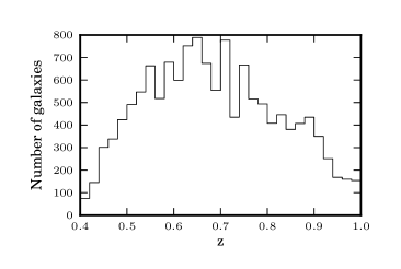
Figure 1: The redshift distribution of the 27,350 VIPERS galaxies used in this study. We have limited the redshift range of the sample to $0.4<z<1.0$, and have applied cuts based on spectral quality.

This study is the first performed on the data of the new VIMOS Public Extragalactic Redshift Survey (VIPERS), the largest redshift survey program currently underway at the European Southern Observatory Very Large Telescope (VLT) (Guzzo et al. 2012, in prep.). VIPERS is designed to map in detail large-scale structure over an unprecedented volume of the $z\sim 1$ Universe.

In this paper, we develop a specific PCA aimed at analysing and classifying the spectra collected by the survey. We show that the technique is capable of compressing the majority of the observed spectral features into a small number of components, allowing an objective classification of the vast majority of the spectra in the sample.

The reasons for doing this on a survey like VIPERS are manyfold. First, it represents a way to objectively classify the survey spectra according to their spectral features. We shall show in the following how true this is by analysing both theoretical models and galaxy templates obtained from observed spectra. A further, important motivation is the possibility to homogeneously define sub-populations of galaxies, to be used for cosmological and evolutionary studies. For example, the analysis of galaxy sub-samples with different bias factors provides a way to reduce the impact of cosmic variance on the measured cosmological parameters (e.g. McDonald & Seljak 2009). A PCA classification can also separate active and passive galaxies, helping to see the effects of environment on galaxy evolution. Furthermore, the classification can be used to help identify, in the VIPERS redshift range, the progenitors of specific populations of galaxies observed in the local Universe, as the Luminous Red Galaxy sample of the SDSS (see for example Wake et al. 2006, Tojeiro & Percival 2010, Tojeiro et al. 2011), or for an analysis of correlation functions in the framework of redshift space distortions (Tojeiro et al., 2012).

The paper is organized as follows: in $\S$2 we present the data and reduction steps; in $\S$3 we introduce the Principal Component Analysis, and the way we implement it as to repair and clean the VIPERS spectra, along with tests on the effectiveness of our routines. In $\S$4 we show the classification obtainable for the VIPERS spectra through this approach and compare it to the results obtained on stellar population synthesis models. In $\S$5 we summarize the results.

2 Data

VIPERS will target $\sim 10^{5}$ galaxies for spectroscopy at redshift $0.5<z\lesssim 1.2$. The sample is selected from the Canada-France-Hawaii Telescope Legacy Survey Wide (CFHTLS-Wide) optical photometric catalogues (Goranova et al., 2009). The target sample covers an area of $\sim 24$ deg² divided over two areas within the W1 and W4 CFHTLS fields. Targets are selected to a limit of $i_{AB}<22.5$ and a colour pre-selection with the $gri$ photometry is used to effectively remove galaxies at $z<0.5$. The detailed description of the target selection can be found in Guzzo et al. (2012) (in preparation).

The spectra are obtained with VIMOS LR Red grism at moderate resolution ($R=210$). The wavelength coverage is 5500-9500$\rm{\AA}$. The data are processed with the Pandora Easylife reduction pipeline (Garilli et al. 2012, in prep.). In this work we utilize flux normalized spectra and variances as well as masks indicating where spurious features in the data have been removed.

Redshifts and quality flags are measured with the Pandora EZ (Easy Z) package (Garilli et al., 2010). The redshift and flag assigned by the Pandora pipeline has been checked and re-fined, for every spectrum, by members of the VIPERS team, ensuring the reliability of the assignments.

The quality flag indicates the confidence of the redshift measurement in a similar manner as used in the VVDS (Le Fèvre et al., 2005) and zCosmos catalogues (Lilly et al., 2007). The flag takes the form $\pm XY.Z$. Negative values are reserved for spurious, undetected or unidentified serendipitous sources. The first digit $X$ indicates the class of object: it is blank for normal galaxies; 1 for broad-line AGNs, and 2 for untargeted sources serendipitously measured. The second digit $Y$ indicates the confidence of the redshift measurement. Secure redshift measurements with nearly 95 per cent confidence are assigned $Y=4$. Measurements with 90 per cent confidence limit are assigned flag 3. Flag 2 measurements have been shown to correspond to a confidence limit of about 80 per cent. Flag 1 sources are highly uncertain at the 50 per cent confidence level, and flag 0 is given when a redshift could not be assigned. For this reason, these two classes are not considered in the present analysis, to guarantee a clean and reliable sample. Finally, flag 9 is given to redshift measurements that are based upon only a single emission line feature. The flag also has a decimal part that indicates the agreement between the photometric redshift estimate and the spectroscopic redshift, but we do not use it here.

The total number of VIPERS spectra available for this first study before any quality cut is 37382, corresponding to the internal data release V2.0 of 23 December 2011. Our further selection excludes low-quality spectra as defined above, but includes sources classified explicitly as broad-line AGN and secondary sources observed by chance. We note that there is no harm in including peculiar spectra as AGN in the overall PCA. Being rare cases, these have no effect on the evaluation of the Principal Components characterizing the main galaxy sample (see § 3). At the same time, as we shall discuss in §4.5, it will be interesting to check how AGN-like spectra can be identified by the PCA as “outliers” among the more standard galaxy spectra. This may lead also to detection of more AGN-like spectra, which do not appear explicitly classified as such.

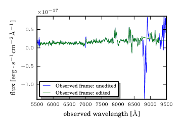
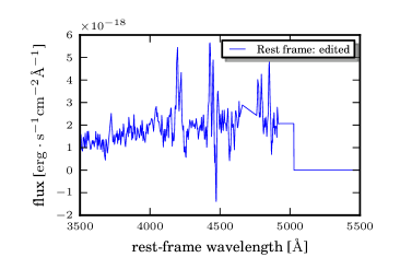
Figure 2: Top: huge noise spike (blue line) due to bad sky subtraction in a VIPERS spectrum at $z\sim 0.88$, and relative edited spectrum (green line). Bottom: The spectrum after resampling on the rest frame wavelength grid. Spurious features have been replaced with a linear interpolation or a flat extrapolation (as in the green spectrum above), and the flux has been set to 0 where no data is available at $\lambda>5000$, due to the shift to the rest-frame.

Since the spectra are observed over a fixed wavelength range, the spectra must be shifted and mapped to a common rest frame wavelength scale. We have defined the rest-frame wavelength scale ranging from $3500<\lambda<5500\rm{\AA}$, to get the maximum coverage in all redshift bins. The redshift range is $0.4<z<1.0$, which covers a large fraction of the redshift range of the survey, excluding very far and very near objects. The final sample, after the cuts, includes 27350 spectra ($\sim 73$ per cent of the total in V2.0). The resulting redshift distribution of the sources used in this analysis is shown in Fig. 1. The wavelength binning we chose to adopt in this work increases logarithmically, such that the last interval in the reddest region has a width of 1$\rm{\AA}$ giving a total number of bins of 2486. This wavelength scale ensures that every VIPERS spectrum is oversampled in the rest frame. The spectra are shifted by a factor of $(1+{\rm z})^{-1}$ and resampled with linear interpolation on to the rest-frame grid. The variance, given for each spectrum by the square of the relative VIPERS noise spectrum, is processed in the same fashion.

Necessarily, resampling a spectrum on to the rest-frame grid can leave gaps at the start or end of the scale, depending on the redshift. Fig. 2 (bottom panel) shows a VIPERS spectrum from a high redshift galaxy after shifting it to the rest frame. No data is available at $\lambda>5000\rm{\AA}$ and in this range the flux is set to 0. Additionally, the VIPERS spectra are affected by fringing redwards of 8000Å induced by the CCD detectors in the VIMOS instrument. The effect was reduced subsequent to the VIMOS refurbishment in August 2010, and about half of the V2.0 sample used here was obtained with the old detector. Fringing can leave strong residuals in the spectrum after sky subtraction, hindering the measurement of spectral features. In some cases, these spikes have been cleaned in the reduction/validation phase, and replaced with a linear interpolation across the spectral region. The presence of these large noise artefacts makes the reconstruction of real spectral features less robust and more complex (Fig.2-Top). For our analysis we would like to develop a procedure to repair these defects. We address this through an iterative algorithm that simultaneously repairs the spectrum and finds the principal components, as suggested in Connolly & Szalay (1999) (see §2.1.).

An important consideration before moving to the analysis is how to normalize each spectrum. The apparent flux of the source introduces an arbitrary scaling factor that should be normalized out to build a homogeneous sample. Amongst many possible normalizations, we choose to normalize each spectrum by a scalar-product normalization, such that for a spectrum $f_{\lambda}$, the normalized spectrum becomes $\overline{f}_{\lambda}=f_{\lambda}/\sqrt{\sum f_{\lambda}^{2}}$. The choice is dictated by the fact that normalizing by scalar product offers advantages for our classification over other possible normalizations (Connolly et al., 1995): a normalization based on morphology would rely on a model distribution of morphological types in given sample, and may lead to the accidental suppression of a common galaxy type within the first principal components of the sample; a normalization by the integrated flux will give similar results as one done by scalar product, in terms of principal components, but this second one produces unit vectors representing the spectra, and unit principal components. This means that the coefficients of the decomposition of each SED on the principal components lie on the surface of an N-dimensional hypersphere (if we consider N principal components), and thus can be parametrized by using only N-1 parameters (see §4.1).

3 The Principal Component Analysis

The Principal Component Analysis (PCA) is a non-parametric way to extract the majority of information from a noisy dataset, composed of objects which are not completely different one from another. The key characteristic of the PCA in this case is, in fact, the ability to describe a large sample through a reduced number of components, which is guaranteed by the fact that the objects in the sample share many common features (e.g. different measurements of the same quantity, a collection of objects in a catalogue, etc…). This holds true for a sample of galaxy spectra that are generated by a common underlying physical mechanism, i.e. the radiative physics in the galaxies.

PCA finds the linear transformation that changes the frame of reference from the observed or natural one to a frame of reference that highlights the structure and correlations in the data. This is done through a rotation of the parameter space such that the axes are aligned along the directions of maximum variance of the data. This transformation may be found by diagonalizing the data correlation (or covariance) matrix, whose eigenvectors effectively represent the axes of the new coordinate system.

The basis of the principal components one obtains will be made up by orthogonal (i.e. uncorrelated) vectors or eigenvectors which are linear combinations of the original variables. The PCA has the advantage to describe a set of measurements exploiting dimensions of the problem which are uncorrelated, and that can be easily ordered by decreasing importance. This allows us to retain just a (small) subset of components, describing the data using a basis of only a few eigenvectors.

Our goal is to reduce the complexity of a sample of spectra by expressing them through just a handful of the principal components. In particular, we may write an observed spectrum as a data vector containing $N$ fluxes $f_{\lambda}$, where $\lambda$ indexes the $N$ wavelength bins. Our sample contains $M$ spectra, and we can write the sample correlation between wavelength bins as a matrix,

$$C_{\lambda_{1},\lambda_{2}}=\frac{1}{M-1}\sum_{i=1}^{M}f_{\lambda_{1}}^{i}f_{\lambda_{2}}^{i},$$ (1)

where $i$ indexes the spectra in the sample and $\lambda_{1}$ and $\lambda_{2}$ index wavelength bins. The correlation matrix can be decomposed into a set of orthonormal eigenvectors, or eigenspectra $e^{i}_{\lambda}$ and eigenvalues $\Lambda_{i}$,

$$C_{\lambda_{1},\lambda_{2}}=\sum_{i=1}^{M}e^{i}_{\lambda_{1}}\Lambda_{i}e^{i}_{\lambda_{2}}.$$ (2)

The eigenspectra are ordered with decreasing eigenvalue such that the most common features within the spectra are contained in the first few eigenspectra.

The eigenspectra form an orthogonal basis or eigensystem and any spectral energy distribution, $f_{\lambda}$, can be expressed as a sum of the $M$ eigenspectra with linear coefficients $a_{i}$:

$$f_{\lambda}=\sum_{i=1}^{M}a_{i}e^{i}_{\lambda}.$$ (3)

Since the higher eigenspectra carry little statistical information about the spectra we may truncate the sum to use only the first $K\ll M$ components. We refer to this as the reconstructed spectrum $\hat{f}_{\lambda}$,

$$\hat{f}_{\lambda}=\sum_{i=1}^{K}a_{i}e^{i}_{\lambda},$$ (4)

The correlation matrix, as defined in (1), will have dimension given by the number of wavelength bins (2486x2486). In the literature, it is also common to define the correlation matrix such that the dimension is the number of spectra (Connolly et al., 1995). This is clearly inefficient when the number of spectra is greater than the number of wavelength bins.

An additional result obtainable by the PCA projection of eq. (4) is a measure of the signal-to-noise ratio for each spectrum, as

$$\frac{S}{N}(f_{\lambda})=\sqrt{\sum_{\lambda}\Big{(}\frac{\hat{f}_{\lambda}}{\overline{n}_{\lambda}}\Big{)}^{2}}$$ (5)

where $\overline{n}_{\lambda}$ is the VIPERS normalized noise spectrum, relative to the spectrum $f_{\lambda}$. Given the VIPERS noise spectrum $n_{\lambda}$, the normalized noise spectrum is given by $\overline{n}_{\lambda}=n_{\lambda}/\sqrt{\sum f_{\lambda}^{2}}$.

3.1 Repairing bad spectral regions

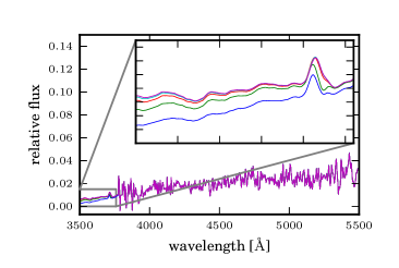
Figure 3: A VIPERS spectrum presenting a gap on the blue side, due to rest-frame shifting. The missing data is reconstructed through an iterative routine. The first five steps (zoomed in the box) go from the first (bottom line) to the fifth iteration (top line).

A spectrum can be corrupted by instrumental artefacts. VIMOS has its own specific features, such as the zero-order image from a bright object in the slit above, or residuals remaining after the subtraction of sky lines. In some cases, artefacts have been removed from the spectra by the reduction pipepline or manually, and have been replaced by linear interpolations, creating “gaps” in the spectra, i.e. regions where flux data was lost. Fig. 2 illustrates a spectrum with a bad region that has been removed. This must be properly taken into account when applying a PCA decomposition, to avoid treating some bad features or noise artefacts as physical peculiarities that will influence the shape of the eigenspectra, and hence the whole analysis. To do that, we assign a weight to each spectral bin

$$w_{f_{\lambda}}=\frac{1}{\overline{n}_{\lambda}^{2}}.$$ (6)

The weight is set to 0 within the gaps and in regions of the spectra that have been manually edited. The weight mask is essential to derive accurate eigen-spectra from data containing gaps. In fact, with a naive application of PCA to these “gappy” spectra, it is no longer possible to construct a set of orthogonal eigenspectra (Connolly & Szalay, 1999). We have therefore developed an algorithm to simultaneously repair the gaps in the spectrum and compute orthogonal eigenspectra.

At the start of the repairing routine, the gaps in the spectra are replaced by linear interpolations. Although, for gaps at the start or end of the spectrum, we find that it is sufficient to simply set the flux to 0. We then proceed in an iterative manner. First, the correlation matrix is constructed from the spectra and the eigenspectra are computed. We keep only the 3 most significant eigenspectra to perform the following repairing steps. The choice of the number of eigenspectra, as discussed later in §3.3, is dictated by the need to be able to describe all the spectra in the sample, while avoiding the noise, which is reflected by the eigenspectra from the fourth on.

We compute the set of eigencoefficients, $\{a_{i}\}$, for each spectrum, $f_{\lambda}$, with a least squares minimization routine. The objective function to be minimized is given by,

$$\chi^{2}=\sum_{\lambda}w_{\lambda}(f^{(i)}_{\lambda}-\sum_{j}a_{j}e_{j\lambda})^{2}.$$ (7)

where $f^{(i)}$ is the spectrum data vector on the $i$^th iteration, $e_{j\lambda}$ is the set of eigenspectra and $w_{\lambda}$ is the weight vector. The minimization is carried out with the Levenberg-Marquardt algorithm implemented in the Python Scientifical Library (Scipy).

We found that in some cases the best-fitting coefficients did not represent physical spectra. For example, the continuum of the repaired spectra could go negative or strong emission lines could be inverted. These poor results are usually found for very noisy spectra or for spectra that are more than 50 per cent masked: in fact, when many spectra have been masked in the same range of wavelengths, the PCA process is unable to find the information to repair the gaps. In our VIPERS sample, there are 57 spectra that are missing more than 50 per cent of the wavelegth coverage, while the average gap fraction for the sample is $\sim 10$ per cent.

The other possibility is that some peculiar piece of information needed to recover a spectrum is not reflected within the chosen eigenspectra (see $\S$2.3).

These problems in the majority of the cases cause the PCA to fail to reproduce simultaneously the continuum and the line features of these spectra, leading usually to the inversion of some lines: the continuum pixels have more weight than those in the lines, and the PCA routine reproduces them as accurately as possible at the expense of the line features. To avoid these degenerate solutions, we introduced a check within the wavelength range of the line features that mostly suffer from this problem in our routine ([OII], H$\beta$ and [OIII]). Whenever the least-square repairing routine finds an inverted line as a solution for the fitting problem, we add an exponential penalty term to the $\chi^{2}$:

$$\chi^{2}=\chi^{2}+c*\sum_{l}e^{(D_{l}-D_{0})/D_{0}}$$ (8)

where $c=$2486 is the number of bins in a spectrum, $D_{l}$ is the difference between the continuum and the line peak for each line $l$, and $D_{0}=$0.005 is the threshold above which the penalty is applied. The value of $D_{0}$ has been chosen such a way to impede the PCA to reverse emission lines, whilst avoiding this penalty to be applied by small real throats within the elected wavelengths, for example in red galaxy spectra. In this way, whenever the PCA finds a negative solution for a real emission line during the phase of repairing, the $\chi^{2}$ gets raised and the routine is therefore forced to find a set of eigencoefficients corresponding to a more physically realistic reparation. The specific choice of this shape for the penalty has been the result of a number of tests using different functions, given the freedom allowed by the problem.

After finding the best-fitting coefficients, $\{\hat{a_{i}}\}$, we reconstruct the spectrum as,

$$y_{\lambda}=\sum_{j}\hat{a}_{j}e_{j\lambda}.$$ (9)

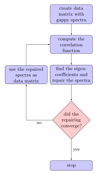
Figure 4: Flow chart of the PCA repairing process.

We then replace the gaps (and only the gaps) in the original spectrum with portions of the projection. In Fig.3 we show an example of different stages of repairing. At each iteration the spectra are renormalized by their scalar products (the normalization changes because the gaps are updated on every loop). The routine progresses as shown in the diagram of Fig (4). Once the eigenspectra of the repaired galaxy sample are obtained (Fig. 8), we can project each spectrum on to the eigenbasis to get the set of eigencoefficients $a_{i}$.

The convergence of the routine is safely reached, for each of the spectra, within the twentieth iteration of the process, when any further refinement of the value of the eigencoefficients for the repairing does not change the repairing significantly, as shown in §3.2.

3.2 Tests with mock spectra

To test our routine we created a synthetic sample of galaxy spectra. The spectra were generated using two sets of templates: a subset of the Bruzual&Charlot (B-C hereafter) (Bruzual & Charlot, 2003) model spectra (which do not contain emission lines), to obtain realistic early-type galaxies, and the 12 Kinney-Calzetti templates (K-C hereafter) (Kinney et al., 1996; Calzetti et al., 1994), covering from pure bulges to starburst galaxies, to give a total of 45 template spectra. We computed the first five eigenspectra of these templates to define an orthogonal basis spanning the range of galaxy types. We then constructed mock spectra that are similar to the templates by generating Gaussian distributed numbers as eigencoefficients. This Gaussian distribution is centered on the first 5 eigencoefficients of the starting template set, with variance given by the relative eigenvalues. We generated 450 mock spectra around each template giving a total sample of 20,250 spectra, that reduces to about 16,000 once spectra presenting unphysical features (i.e. inverted emission lines) are removed.

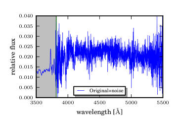
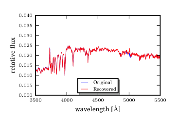
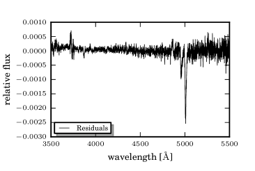
Figure 5: Top: a synthetic spectrum with synthetic noise added. The shaded region would be masked and reconstructed. Middle: qualitative comparison between the original spectrum before the noise has been added (blue) and its reconstruction through the PCA routine (red). Bottom: residuals between the mock and its reconstruction. The possible differences between the intensities of the real and the recovered emission lines are acceptable for our classification system, since it is more sensitive to the continua of the spectra than to the line features.

We next degrade the spectra with synthetic noise to simulate the VIPERS data. Each synthetic spectrum is assigned the same data variance and weight mask of a randomly selected VIPERS galaxy. The synthetic noise spectra are generated from a Gaussian realisation with the associated VIPERS variance, as illustrated in the top panel of Fig.5, and the mask is applied to reproduce the gaps. In this way, we produce an artificial data set that can be used to test the fidelity of the reconstruction procedure.

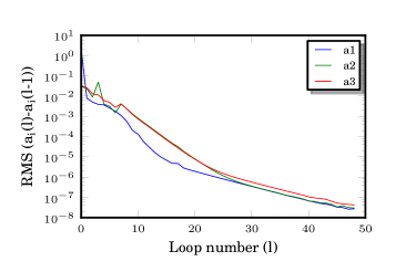
Figure 6: The root mean square difference between the eigencoefficients and themselves at the previous iteration, for the repairing of the synthetic spectra. The RMS difference steadily decreases on subsequent iterations.

We apply the PCA repairing routine with three eigenspectra. Then we project the spectra on them, to clean from noise and be able to compare the recovered spectra to the noise-free synthetic ones. Apart from slight differences in the intensity of the emission lines (as anticipated in §3.1) the reconstruction is qualitatively good, even where the region to be repaired was a line feature (Fig.5: middle-bottom, Fig. 6 for a more quantitative check) . The fit can be improved by adding more components to the PCA, but, as will be discussed later, the 4th eigenspectrum is already affected by noise for the VIPERS sample, and the reconstruction obtained with three is sufficient for the classification system.

The PCA routine has been run on the synthetic spectra for a large number of iterations, that we chose to be 50. By looking at the root mean square difference between the eigencoefficients at each iteration (Fig. 6) we see that the routine is converging: in particular, the differences between the eigencoefficients become steadily smaller. The effects of this on the repairing is actually negligible after five iterations, so we halt the code when the difference between the eigencoefficients at consecutive loops is $\leq 10^{-3}$, since under this threshold further refinement has a negligable effect on the results. We found that the repairing for every single spectrum has surely reached $10^{-3}$ within the 15th iteration for $a_{1}$, at the 17th for $a_{2}$ and at the $16$th for a₃, so in this case 17 iterations are enough to repair and recover the original spectra for the synthetic spectra. To be on the safe side, we decide to take 20 iterations.

3.3 VIPERS spectra: repairing and cleaning

We now apply the PCA routine to the VIPERS sample. As anticipated in sections $\S\ref{sec:rep}$ and $\S\ref{sec:tests}$, we must decide on a stopping point for the repairing routine and the number of eigenspectra to use.

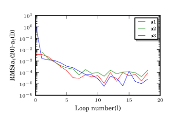
Figure 7: The RMS error on coefficients for VIPERS spectra. Plotted is the root mean square difference of the coefficients of the decomposition after 20 iterations, and themselves at the $i^{\rm th}$ iteration. For a particular spectrum the difference actually starts oscillating around 0 with decreasing amplitude after the 5-10th iteration on average.

As suggested by the tests on mock spectra, we halt the repairing procedure after 20 iterations. We may estimate the relative error in the coefficients after each iteration by measuring the root mean square difference between the value at iteration $i$ and iteration 20. Fig. 7 shows that this error is oscillating at the level of $10^{-4}$ by the 10^th iteration.

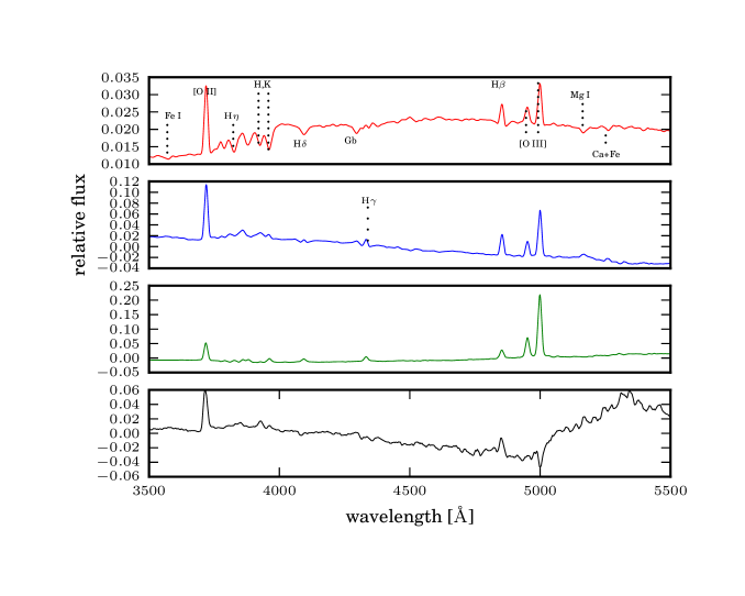
Figure 8: The first four VIPERS eigenspectra computed after repairing. From top to bottom the power is decreasing (the first eigenspectrum is at the top, the fourth at the bottom). The first eigenspectrum mirrors the average of all the spectra, while the second and the third are residuals form the average. Some of the most common spectral features present in the eigenspectra are highlighted in the first eigenspectrum. Systematic effects in the spectra begin to be visible in the fourth spectrum at $\lambda>5000$Å

We use three eigenspectra in the repairing procedure to reconstruct the spectra inside the gaps. This number should be chosen to be large enough such that the repairing can reproduce the signal without adding spurious noise, although the results are not strongly dependent on the exact number used.

After the convergence of the repairing process, we obtain the complete eigenspectra for the VIPERS sample. The first four eigenspectra ordered by significance are shown in Fig. 8. The first three VIPERS eigenspectra, as shown, contain the large majority of information on the sample, particularly the first one, which mirrors the average of all the spectra, while the others represent the residuals from the mean. In particular, the shape of the continuum of the first eigenspectrum is comparable to the one of an early-type galaxy, while it contains also emission lines typical of a star-forming galaxy. The second one instead can be associated to a late-type spectrum, while the third can be thought of as an intermediate galaxy SED. The fourth one, at $\lambda<4500$Å, adds information about the intensity of the [OII] emission line and the continuum resembles the one of a blue galaxy, but redward of 4700 Å  it shows an unphysical bump that is not expected in a galaxy continuum. We attribute this to the fact that, redwards of $\lambda_{obs}>8000$Å , VIPERS spectra are affected by systematic effects arising from the coupled effect of detector fringing and strong sky emission lines (Guzzo et al. 2012, in prep.). For low signal-to-noise objects the repairing of this region is probably more affected by systematic uncertainties that can heavily influence the PCA reconstruction. Thus, to effectively repair the spectra without spurious features, we use only the first three eigenspectra.

By a simple estimate of the power enclosed in each eigenspectrum

$$P(e_{i})=\frac{\Lambda_{i}}{\sum_{i=1}^{tot}\Lambda_{i}},$$ (10)

where $\Lambda_{i}$ are the eigenvalues of the correlation matrix, we find that the first three eigenspectra hold $\sim$ 90.6 per cent of the total power; the first contains $\sim$ 87.3 per cent, the second $\sim$ 2.5 per cent, the third $\sim$0.7 per cent, and from the fourth on the power content starts to decrease rapidly with respect to the first three, see Table 1. The variance in each component is a measure of the information content and we can conclude that three eigenspectra are enough to describe the sample in a statistical sense. However, we will see that this measure of information does not translate directly to the physical information contained in spectral features, as anticipated in §3.1. For example, we found that the slope of the continuum is well described by just a few eigenspectra, but this is not true for the line features. The information on the lines in some cases is contained into higher-order components, that we neglect to avoid the noise, even though we recognize that this information is essential for understanding the physical properties of galaxies.

Power of the first three eigenspectra	$\sim 90.56\%$
First eigenspectrum	$\sim 87.30\%$
Second eigenspectrum	$\sim 2.54\%$
Third eigenspectrum	$\sim 0.71\%$
Fourth eigenspectrum	$\sim 0.17\%$

Table 1: The power contained in the first four eigenspectra.

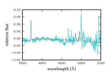
Figure 9: Two repaired and cleaned VIPERS spectra (red) superposed to themselves after the only repairing process (cyan). Our projection method is statistically able to recover the realistic emission and absorption features together with the slope of the continuum. This is a consequence of the combination of “cleaning”, operated by the description of the spectra through the first three eigenspectra, which do not reflect the noise of the sample, and least-square fitting with introduction of penalty terms in the regions of the lines.

After the repairing process, by projecting the VIPERS spectra on to the basis of three final eigenspectra we can achieve our goal of cleaning the spectra from noise, as illustrated in Fig. 9. This is guaranteed by the fact that the first three eigenspectra are affected very little by noise. The same simplification offered by the PCA in using only three components makes it impossible, though, in our specific case, to naively apply Eq. (4) to recover properly VIPERS spectra. In fact, as for the repairing process, the projection on to only a few components is not guaranteed to reproduce spectral features matching the data. And again, as for the repairing, the projection can invert lines or add lines not present in the data. These errors arise because additional components are needed to recover all the lines accurately. We find that 5 per cent of spectra show unphysical line feaures once projected on to 3 components only. The situation can be improved by adding more components to the projection; however, this will re-introduce noise and artefacts, again degrading spectral features.

We can arrive at a compromise by assigning greater importance to the physical recovering of emission lines. This is precisely what was done in §3.1 where penalty terms were added in the least-squares minimization procedure to find the best-fitting, but physical repairing. We adopt this routine again in the final step to project each spectrum. The safeguard of the physicality of spectra is constrained imposing that the continuum is positive and the [OII], H$\beta$ and [OIII] lines are not inverted. By comparison of the equivalent width of the [OII] line in the repaired and projected spectra to the same feature in the original spectrum, we find that the line, on average, is recovered with a precision of $\sim 20$ per cent, whereas for $\sim 68$ per cent of the spectra the line is recovered within 10 per cent. This is in agreement with the results found by Yip et al. (2004) for the majority of SDSS spectra in their analysis with 3 eigenspectra. For the reconstruction of the problematic emission line spectra only, they chose instead to use 10 eigenspectra, obtaining an error on the recovering of the lines of order 15-25 per cent. Finally, the final quality of the repairing in our analysis, after the penalty has been applied, doesn’t show any clear correlation to the portion of gaps in a spectrum, even if larger gaps easily increase the possibility of unphysical reconstructions at first step.

4 Classification of VIPERS spectra

4.1 K-L Projection

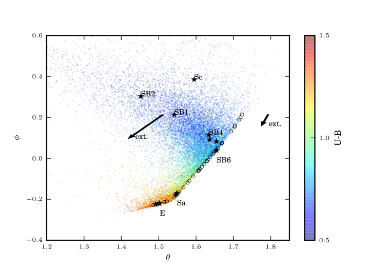
Figure 10: The K-L plot, $\phi$ versus $\theta$, for VIPERS repaired and cleaned galaxies, with the position of Bruzual-Charlot and Kinney-Calzetti model galaxies overplotted. The colour gradient of the points from red to blue through green represents the $U-B$ rest frame color of each galaxy in the sample. The sequence of circle markers represents the B-C models ranging from the reddest (early-type) to the bluest (late-type) continuum slopes. The Kinney-Calzetti templates (star markers) are labelled with galaxy type. The early type galaxies are positioned with the early-type B-C templates, while the starburst templates are found in the middle. The sharp edges in the distribution on the right hand side arise from constraints applied in the PCA reconstruction. Finally, the arrows show the effects of dust extinction for the two sets of models, with $A(V)$=1 mag and $R_{V}$=3.52.

The eigen-coefficients $a_{1}$, $a_{2}$ and $a_{3}$ form an optimal basis in which to classify the spectra. To further reduce the parameter space to a non-degenerate basis we compute the Karhunen-Loève angles (K-L hearafter) (Connolly et al., 1995; Karhunen, 1947; Loève, 1948), so defined:

$$\phi=\tan^{-1}\Big{(}\frac{a_{2}}{a_{1}}\Big{)}$$ (11)

$$\theta=\cos^{-1}a_{3}$$ (12)

The two angles $\phi$ and $\theta$ fully parametrize the three dimensional space because, owing to the normalisation constraint, the coefficients fall on the surface of a 3D sphere.

Figure 11: The B-C spectra corresponding to the circles in Fig. 10: red templates (bottom) lie in the low-$\phi$ region, with intermediate templates instead occupying the range $-0.2<\phi<0$ (middle boxes), and bluer ones lying at the top of the K-L plot.

To pin down the location of different galaxy types on the $\phi-\theta$ plane, we take advantage of the same group of B-C model spectra from which we picked the templates used to test the repairing routine (keeping also the blue galaxy representatives, although these are not fully realistic because of the lack of emission lines). We project them on the three VIPERS eigenspectra and then obtain the K-L angles, which are shown in Fig. 10.

We find that in the K-L plot, the redder galaxies lie towards negative values of $\phi$ and quite small values of $\theta$, while, as $\phi$ and $\theta$ increase, the galaxies become bluer (Fig. 11), as suggested by the $U-B$ rest-frame color of VIPERS galaxies. Since an increase in $\phi$ is equivalent to an increase in $a_{2}$, this means that the bluer galaxies are represented by larger values of $a_{2}$ (and viceversa for the redder ones). This is expected, since the shape of the second eigenspectrum is the one that most resembles the spectrum of a blue galaxy. We do not consider now the first eigencoefficient $a_{1}$, because, being related to the first eigenspectrum, which is the average of all the spectra, it is not a significant discriminator. Let us remark again, though, that we are basing this interpretation on a set of model spectra that do not present emission lines, although they do trace the continuum of blue galaxies in some cases. So they give a general idea of the arrangement of different spectral types on the K-L plot, but they are not apparently able to span the full distribution.

To get more quantitative information on how galaxies spread on the K-L plane, we performed the same comparison using the Kinney-Calzetti templates (Fig. 10). These are the same we used in §2.2 to build the synthetic spectra for the test, together with the B-C red-intermediate spectra.

The K-C templates provide confirmation that the earliest type galaxies are at the bottom of the K-L plot, as suggested by the bulge and elliptical K-C templates. Additionally, the K-C-Sa and K-C-Sb spiral galaxies fall near to the region of intermediate B-C models, consistent with them presenting a certain level of star formation. The starburst galaxies, instead, follow a branch which is nearly orthogonal to the trend followed by red and intermediate galaxies. Finally, the K-C-Sc template occupies the highest position in $\phi$ in the plot, due to the steepness of its continuum, and it is more shifted towards lower values of $\theta$ with respects to B-C models, due to the presence of emission lines. We also found that moving towards lower values of $\theta$ corresponds to increase the intensity of emission lines; this will become evident in section §4.3. So we can state that the two K-L parameters $\phi$ and $\theta$ are related to the age and to the star-formation-rate in a rather complex way: an age sequence can be observed moving along the direction of the ridge of normal galaxies, at the right edge of the K-L plot, while an instantaneous star formation sequence can be observed on the perpendicular direction.

The sharp bottom and right edges of the cloud of data points in the K-L plane are a consequence of the least-square penalty terms, introduced in the projection of the sample over the eigenspectra basis, together with the limits imposed by our two-components parametrization. These two boundaries limit forbidden regions beyond which the reconstructions would be unphysical with negative continua or inverted emission lines due to the possible lack of information of the chosen components, if the penalty was not applied. Consequently, spectra with no emission lines are found at these edges of the cloud of points, as demonstrated by the B-C models.

4.1.1 Comparison to SDSS data

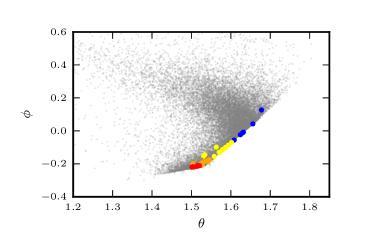
Figure 12: The set of 38 SDSS templates by Dobos et al. (2012) as projected on the VIPERS eigenspectra. The templates roughly follow the evolutionary track marked by the right edge of the K-L plot, apart from 3 templates that present stronger emission lines in the red part.

We can compare the distribution of VIPERS galaxies to SDSS galaxies on the K-L plot. To this purpose, we used a set of 38 SDSS templates computed through a PCA projection by Dobos et al. (2012). The templates were first re-binned on the same wavelength scale of VIPERS data, and normalized through their scalar product. They were then simply projected on the VIPERS first 3 eigenspectra with the same routine discussed earlier.

The SDSS templates fall in the region at the right edge of the plot, following the same track found for the other datasets. In particular, the majority of them can be found near to the right sharp edge, because their PCA projection over the VIPERS first 3 eigenspectra was finding unphysical solutions for the line features and needed the $\chi^{2}$ penalty to be applied. The colour gradient, from red to blue, gives a qualitative idea of the colour of the relative template (Fig. 12). Only a group of three spectra seem to detach from the main branch, positioning in a region of slightly smaller $\theta$. The reason for that, as expected, is that those spectra present slightly stronger emission lines, mainly in the red part, than all the other SDSS templates. Again, the PCA proves much more sensitive to the slope of the spectra than to emission lines in positioning the objects on the $\phi$ scale. In fact, although the blue templates present strong emission lines, their slope is flatter than many VIPERS blue galaxies, causing the templates to hardly reach large numbers in $\phi$.

4.2 Effect of dust

A natural question we can now ask about our classification regards the effects of dust extinction on the position in the K-L plot. To this end, we applied an extinction law to the model templates. Since our purpose is only to check the direction to which extinction moves the galaxies in the K-L plot, we chose to apply the same simple Cardelli-Clayton-Mathis extinction laws (Cardelli, Clayton and Mathis, 1989) to all galaxy types, over the optical-near infrared wavelength range ($3000\mathrm{\AA}\leq\lambda\leq 9000\mathrm{\AA}$), which contains the rest frame range we considered for our VIPERS data. The parameter $R_{V}[=A(V)/E(B-V)]$, with $A(V)$=1 mag, was set to 3.52. The extinction effects on the B-C and Kinney-Calzetti models are represented by the arrows shown in Fig. 10.

Once the B-C models have been corrected for dust-extinction, they all shift towards the bottom of the K-L plot (Fig. 10), in the same direction marked by the B-C curve. This is consistent with a reddening of the continuum. For the Kinney-Calzetti templates, and in particular for the starburst spectra, we find that dust extinction causes a larger shift within the K-L plot than for B-C spectra, probably due to the fact that young or starburst galaxies have a higher gas content; this explains also why the points in that region of the K-L plot display a broader distribution: because of the higher gas content of the galaxies represented in that region, extinction causes larger shifts in the intensity of emission lines and in the slope of the continua.

4.3 Spectral sequence

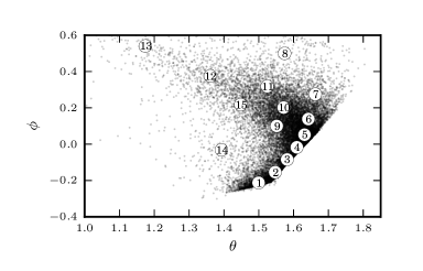
Figure 13: K-L plot of VIPERS repaired and cleaned galaxies, labelled with numbers 1-15, that represent the diversity of spectral types. The primary locus is traced by markers 1-8, and we find a secondary branch, marked 9-13. The mean spectrum at each marker is plotted in Fig. 15.

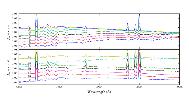
Figure 14: Representative average spectra obtained by grouping the VIPERS spectra through a group-finding algorithm into 15 classes in the $(\theta,\phi)$ plane, as labelled in Fig. 13. We average the repaired and cleaned spectra (i.e. considering only the three principal components). In the top frame, we show that spectra 1-8 follow a sequence from early to late types, with the continuum becoming progressively bluer and with stronger [OII] emission. Note that the spectrum labelled as 1, i.e. the reddest one, still presents a hint of emission lines (although pure red spectra exist in the sample), since it is an average spectrum. In the bottom frame, spectra 9-13 represent starburst galaxies with flatter continua and strong emission lines. Mean spectra 14-15 effectively seem to pertain to none of the two branches, showing a mixture of blue and red galaxy properties.

To explore the diversity of spectra represented on the K-L plot, we apply a k-means group-finding algorithm that partitions the space into maximally diverse classes (Ascasibar & Sánchez Almeida, 2011). Galaxies are associated with a group based upon the distance in the $\theta-\phi$ coordinates. It is necessary to specify the number of groups beforehand, and we chose 15, which appear to be sufficient to span all features visible by eye.

The positions of the classes we have identified are marked in Fig. 13. These points trace out essentially two branches that can be thought of as the skeleton of the data cloud. The first branch, marked by the numbers 1-8, shows a sequence very similar to what we can imagine as the prosecution of the B-C red and intermediate models discussed previously, encompassing though also the starburst galaxies type 3-4-5-6. In particular, the Sc template appears to lie between the 7 and 8 classes. A second branch, marked by 9-13, lies almost perpendicular and passes through the starburst 1-2. The mean spectrum that represents each class is plotted in Fig. 14. In particular, in the top panel of Fig. 14, we see that moving from 1 to 8 means an increase in the intensity of emission lines and a change in the slope of the continuum, from redder to bluer. In the bottom panel of Fig. 14, mean spectra from 9 to 13, pertaining to the perpendicular “starburst” branch, show an increase in the intensity of emission lines, particularly evident by looking at the H$\gamma$ emission, while the slope of the continuum is substantially unchanged.

Consecutive numbers here label very similar average spectra in almost all cases, apart from spectra 14-15, which do not resemble spectrum 13. Mean spectra 14-15 in fact, lying beyond the imaginary starburst branch in Fig. 13, actually don’t follow the trend of that branch, but show redder continua, in agreement with their $\phi$ position on the K-L plot. They look more similar to mean spectra 3 and 7 respectively, but for the intensity of emission lines, since they exhibit stronger line features. The combination of red continua and strong emission lines shown by mean spectra 14-15, makes them hardly includable in any of the two branches. This suggest that, while moving upwards in the $\phi$ direction in the K-L plot can be associated to a change in the slope and the intensity of the lines, moving from right to left in the $\theta$ direction also means a strengthening in the intensity of the emission lines.

The shape of the mean spectra for the different groups and the position of the same groups on the K-L plot reinforce the evidence that galaxies can be to split into two nearly orthogonal spectral sequences, of which one reflects the evolutive phases of a normal galaxy (though not being an evolutionary track), while the other describes the starburst phases. This suggests a route for building a physical classification of the spectra based on the K-L parameters, which we plan to develop in a future work.

4.4 Comparison with photometric classification

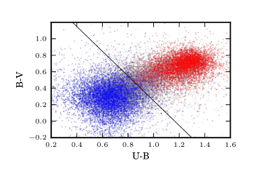
Figure 15: The rest frame $U-B$, $B-V$ colours of VIPERS galaxies. Red points have PCA parameter $\phi<-0.1$ and blue points have $\phi>0.1$ (intermediate values of $\phi$ are coloured grey). The line dividing the two samples optimally separates $\phi>0$ from $\phi<0$ in colour space with a contamination of $\sim 13$%.

Finally, we compare side by side the PCA classification against the more familiar one based on rest-frame broad-band photometric colours. In Fig. 15 we plot the VIPERS rest-frame $U-B$ and $B-V$ for each galaxy (Bolzonella et al., in prep, Fritz et al., in prep.). We divide the sample into red and blue classes using the K-L angle $\phi$. Based on the comparison to the model spectra and the discussion of the previous section, a reasonable definition of the red class can be $\phi<-0.1$, with the blue galaxies confined at $\phi>0.1$. In this way, we cleanly exclude intermediate types.

For comparison, we construct a red-blue classification using the $U-B$ and $B-V$ colours that match as well as possible the PCA selection. This is shown in Fig. 15, where the two classes defined through the K-L angle are plotted in blue and red and the intermediate types in grey. We clearly note that the PCA selection is correctly capturing the bimodal distribution. Conversely, let us verify how a crude color-color selection performs, with respect to that based on the spectral information “compressed” into the PCA parameters. We therefore separate photometrically red and blue classes by tracing a line perpendicular to the axis connecting the centres of the two clouds, (Fig. 15). This axis is defined by computing, through a simple PCA, the two eigenvectors of the distribution of points on the colour plane: the first eigenvector marks the principal direction of the data, while the second is orthogonal to the first one. Here the total number of eigenvector is only two, since the correlation matrix of a two-dimensional distribution has dimension 2. The position of the line is set such that there is an approximately equal number of contaminating galaxies on the red and blue sides. With respect to the PCA classification, we find that: (1) in selecting red galaxies, the color-color selection has a $\sim 14$ per cent contamination of spetroscopically blue galaxies and an $\sim 88$ per cent completeness; (2) for photometrically blue galaxies, the contamination of objects that spectroscopically are classified as “red” is $\sim 12$ per cent and the completeness is $\sim 86$ per cent.

It is encouraging that in this simple case of classifying galaxies as red or blue, the two methods produce very similar results. The strength of the PCA approach is that it encodes additional information about spectral features that is not available in the broad band photometry.

4.5 Outliers

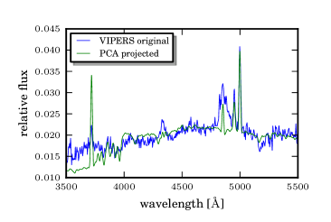
Figure 16: Example of an AGN in the VIPERS sample (blue) projected on to the PCA eigenspectra basis (green). The PCA reconstruction was not able to preserve the peculiarities of this rare spectrum, forcing it to resemble a typology of galaxy which is much more common within the VIPERS sample.

One of the limitations of the PCA reconstruction of spectra is that a spectral type that is represented by a few galaxies only will be poorly (or even will be not) represented by principal eigenspectra. Rare features will not be included in the main eigenspectra, but only in higher-order ones.

This is for example the case of AGNs (as QSOs or Seyfert galaxies; it can be also the case of normal galaxies which have been assigned a wrong redshift). Their representation, in terms of the first three components only, will not be realistic. This will force them to resemble an intermediate, blue, or starburst galaxy. An example is shown in Fig. 16, where a broad-line AGN is reconstructed using only three eigenspectra. The continuum is approximately fitted, but the broad emission features do not have counterparts in the three basis vectors used.

We have directly verified that AGN features start to emerge only when principal components up to orders $\gtrsim$ 50 are included. This is due to the fact that AGNs are actually a minority in the VIPERS catalogue (we expect them to be $\sim 5$ per cent of the total), so their peculiar features are treated as “noise” (i.e. uncommon features) by the PCA. For these reasons the AGNs do not group as a separate population of outliers in the K-L plot computed with three or higher-order eigenspectra, but fall on the main locus in apparently random positions. A PCA reconstruction of the AGN spectra will be better performed when a larger sample of AGNs only will be available. On the other hand, given a large data set like VIPERS, for the same reasons the PCA allows us to identify rare objects (as the AGN in this case) or even to look for previously unknown types.

One could use the goodness of fit $\chi^{2}$ value to isolate spectra that are poorly represented by the principal eigenspectra. When the $\chi^{2}$ is larger than a given threshold, we know that the original is poorly traced by the projection. A large $\chi^{2}$ depends also on the signal-to-noise ratio of the original spectrum. Thus, isolating the spectra presenting a high $\chi^{2}$ together with a reasonably high signal-to-noise (as defined in Eq. 5) will select highly-confident outliers. It will be interesting to explore the application of this technique to a future, larger version of the VIPERS catalogue and compare it to alternative methods.

5 Summary and Conclusions

We have developed an objective spectral classification system based on a principal component analysis for the ongoing VIPERS survey. Here, we present the analysis of the first sub-set consisting of 27,350 galaxy spectra at redshifts $0.4<z<1.0$. Our implementation of a principal component analysis addresses the non-uniform characterstics of the dataset that can impede the measurement and classification of spectral features, including the variation of wavelength coverage in the rest frame, noise properties and instrumental artefacts. We correct for these effects using an iterative algorithm that converges to a robust estimate of the eigenspectra templates.

Our final classification system is based upon three coefficients, $a_{1}$, $a_{2}$ and $a_{3}$, that are found by projecting the spectra on to the first three principal components. The determination of the coefficients for each spectrum uses a specific recipe to preserve the physicality of spectral lines such that both the continuum and line features are reconstructed accurately. The first three eigencoefficients provide a high-fidelity reconstruction of the spectrum for a broad range of galaxy types.

The information enclosed in the three eigencoefficients can be compressed in the K-L angles representation: $\phi=\tan^{-1}(a_{2}/a_{1})$ and $\theta=\cos^{-1}a_{3}$. This is a key step for our spectral classification: in a $\theta$–$\phi$ plane galaxies of different colour concentrate in different regions, according to the relative importance of the three eigenspectra. These, at least in terms of the continuum, mirror the shape of realistic red, blue and intermediate galaxies.

To explore the physical meaning of the different positions on the $\theta$–$\phi$ diagram, we projected a set of Bruzual-Charlot model spectra on the same VIPERS eigenspectra and looked at their distribution on the same plot. We also added a set of 12 Kinney-Calzetti templates, as to verify the appearance of starburst galaxies over the same plane. An analysis with a group finding algorithm capable to divide space into maximally diverse classes, showed clear evidence of two different branches, following respectively the trend of the Bruzual-Charlot and Kinney-Calzetti models. The models have been also dust extincted to know in which direction the reddening for spectra moves the points in the K-L cloud.

A comparison of our classification method with a more common photometric selection shows that the PCA approach is comparable to a rest-frame color-color plot in discriminating red from blue galaxies, whereas being more sensitive than photometry to intermediate spectral types, being based on spectra.

Some peculiar spectra will not be well represented in the eigenspectra, due to the rareness of their features in the sample. For instance, we find that the eigenspectra do not fit AGN spectra well. However, in principle, interesting outlying spectra can be identified based upon poor $\chi^{2}$ values for the fit.

We remark that we have analysed only the initial 40 per cent of the VIPERS survey. As the data sample increases and the statistics grow, the repairing procedure will improve in precision. In future analyses we will have the possibility to divide the sample in redshift bins. Additionally, the analysis can be naturally extended to include additional observations, such as galaxy luminosities and broadband fluxes.

References

- Abbas et al. (2010) Abbas U., et al., 2010, MNRAS, 406: 1306
- Ascasibar & Sánchez Almeida (2011) Ascasibar Y., Sánchez Almeida J., 2011, MNRAS, 415, 3: 2417-2425
- Baldry (2004) Baldry I.K., 2004, ApJ 600: 681
- Bell et al. (2004) Bell E.F., 2004, ApJ, 608: 752
- Blanton et al. (2003) Blanton M.R., et al. 2003, ApJ, 594: 186
- Brammer et al. (2009) Brammer G.B., et al., 2009, ApJ, 706L: 173
- Bromley et al. (1998) Bromley B.C., Press W.H., Lin H., Kirshner R., 1998, ApJ, 505: 25
- Brown et al. (2003) Brown M.J.I., Dey A., Jannuzi B.T., Lauer T.R., Tiede G.P., Mikles V.J., 2003, ApJ, 597: 225
- Bruzual & Charlot (2003) Bruzual G., Charlot S., 2003, MNRAS, 344,4: 1000-1028
- Cabré & Gaztañaga (2009) Cabré A., Gaztañaga E., 2009, MNRAS, 393: 1183
- Calzetti et al. (1994) Calzetti D., Kinney A.L., Storchi-Bergman T., 1994, ApJ, 429: 582
- Cardelli, Clayton and Mathis (1989) Cardelli J.A., Clayton G.C., Mathis J.S., 1989, ApJ, 345: 245, 256
- Cimatti et al. (2002) Cimatti A., et al., 2002, A&A, 381L: 68
- Coil et al. (2006) Coil A.L., Newman J.A., Cooper M.C., Davis M., Faber S.M., Koo D.C., Willmer C.N.A., 2006, ApJ, 644: 671
- Coil et al. (2008) Coil A.L., et al., 2008, ApJ, 672: 153
- Connolly et al. (1995) Connolly A.J., Szalay A.S., Bershady M.A., Kinney A.L., Calzetti D., 1995, ApJ, 110,3: 1071-1082
- Connolly & Szalay (1999) Connolly A.J., Szalay A.S., 1999, ApJ, 117: 2052-2062
- Coupon et al. (2012) Coupon J., et al., 2012, A&A, 542A: 5
- Daddi et al. (2003) Daddi E., et al., 2003, ApJ, 588: 50
- Davis & Geller (1976) Davis M., Geller Margaret J., 1976, ApJ, 208: 13
- de la Torre et al. (2011) de la Torre S., et al., 2011, MNRAS 412, 2: 825-834
- de Vaucouleurs (1962) de Vaucouleurs G., 1962, Problems of Extra-Galactic Research, Proceedings from IAU Symposium no. 15. Edited by George Cunliffe McVittie. International Astronomical Union Symposium no. 15, Macmillan Press, New York, p.3
- Dobos et al. (2012) Dobos, L., Csabai, I., Yip, C.-W., et al., 2012, MNRAS, 420: 1217
- Faber et al. (2007) Faber S.M., et al., 2007, ApJ, 665: 265
- Ferreras et al. (2006) Ferreras, I., Pasquali, A., de Carvalho, R. R., de la Rosa, I. G., & Lahav, O., 2006, MNRAS, 370: 828
- Folkes et al. (1996) Folkes S., Lahav O., Maddox S.J., 1996, MNRAS, 283: 651
- Francis et al. (1993) Francis P.J., Hewett P.C., Foltz C.B., Chaffee F.H., 1993, ApJ, 398: 476
- Franzetti et al. (2007) Franzetti P., et al., A&A, 465: 711
- Galaz & de Lapparent (1998) Galaz G., de Lapparent V., 1998, A&A, 332: 459
- Garilli et al. (2010) Garilli B., Fumana M., Franzetti P., Paioro L., Scodeggio M., Le Fèvre O., Paltani S., Scaramella R., 2010, PASP
- Gavazzi et al. (2003) Gavazzi G., Boselli A., Donati A., Franzetti P., Scodeggio M., 2003, A&A, 400: 451
- Giovanelli et al. (1986) Giovanelli R., Haynes M., Chincarini G.L., 1986, ApJ, 300: 77
- Goranova et al. (2009) Goranova Y., Hudelot P., Magnard F., et al., 2009, The CFHTLS T0006 Release, http://terapix.iap.fr/cplt/table_syn_T0006.html
- Graves et al. (2007) Graves Genevieve J., Faber S.M., Schiavon Ricardo P., Yan Renbin, 2007, ApJ, 671: 243
- Guzzo et al. (1997) Guzzo G., Strauss M.A., Fisher K.B., Giovanelli R., Haynes M.P., 1997, ApJ, 489: 37
- Karhunen (1947) Karhunen H.., 1947, Ann. Acad. Science Fenn, Ser. A.I. 37
- Kinney et al. (1996) Kinney A.L., Calzetti D., Bohlin R.C., McQuade K., Storchi-Bergman T., Shmitt H.R., 1996, ApJ, 467: 38
- Le Fèvre et al. (2005) Le Fèvre O., et al. 2005, A&A, 439: 845
- Lilly et al. (2007) Lilly S.J., et al., 2006, ApJ Supplement Series, 172, 1
- Loève (1948) Loève M., 1948, Processus Stochastiques et Mouvement Brownien (Hermann, Paris, France)
- McDonald & Seljak (2009) McDonald P., Seljak U., 2009, jcap, 10, 7
- Maddox et al. (1998) Maddox S.J., et al., Large Scale Structure: Tracks and Traces, ed. Muller (Singapore: World Scientific), 99
- Madgwick et al. (2002) Madgwick D.S., et al. 2002, MNRAS, 333: 133
- Madgwick et al. (2003) Madgwick D.S., Coil, A.L., Conselice C.J., Cooper M.C., et al. 2002, MNRAS, 333: 133
- Mendez et al. (2011) Mendez A.J., Coil A.L., Lotz J., Salim S., Moustakas J., Simard L., 2011, ApJ, 736, 2: 110-133
- Meneux et al. (2008) Meneux B., et al., 2008, A&A, 478: 299
- Meneux et al. (2009) Meneux B., et al., 2009, A&A, 505: 463
- Morgan & Mayall (1957) Morgan W.W., Mayall N.U., 1957, Publications of the Astronomical Society of the Pacific, 69, 409 : 291-303
- Norberg et al. (2002) Norberg P., et al., 2002, MNRAS, 332: 827
- Phleps et al. (2006) Phleps S., Peacock J.A., Meisenheimer K., Wolf C., 2006, A&A, 457: 145
- Ronen, Aragon-Salamanca and Lahav (1999) Ronen S., Aragón-Salamanca A., Lahav O., 1999, MNRAS, 303: 284
- Rogers et al. (2007) Rogers, B., Ferreras, I., Lahav, O., Bernardi M., Kaviraj S., Yi S.K., 2007, MNRAS, 382: 750
- Rogers et al. (2010) Rogers, B., Ferreras, I., Pasquali, A., Bernardi M., Lahav O., Kaviraj S., 2010, MNRAS, 405: 329
- Singh, Gulati and Gupta (1998) Singh H.P., Gulati R.K., Gupta R., 1998, MNRAS, 295: 312
- Sodre & Cuevas (1997) Sodre L., Cuevas H., 1997, MNRAS, 287: 137
- Strateva et al. (2001) Strateva I., Ivezić Ž., Knapp G. R., et al. 2001, AJ, 122: 1861
- Tojeiro & Percival (2010) Tojeiro R., Percival W.J., 2010, MNRAS 405: 2534-2548
- Tojeiro et al. (2011) Tojeiro R., Percival W.J., Heavens A.F., Jimenez R., 2010, MNRAS 413: 434-460
- Tojeiro et al. (2012) Tojeiro R., et al., 2012, preprint (astro-ph/1202.6241)
- Sandage (1975) Sandage A.R., 1975, Stars and Stellar Systems, Vol. 9, Galaxies and the Universe, ed. A.R. Sandage, M.Sandage, and J. Kristian (Chicago: University of Chicago Press), p. 761ff
- Wake et al. (2006) Wake D.A., Nichol R.C., Eisenstein D.J., et al., 2006, MNRAS 372: 537-550
- Weiner et al. (2005) Weiner B.J., et al., 2005, ApJ, 620: 595
- Yip et al. (2004) Yip C.W., Connolly A.J., et al., 2004, ApJ, 128: 585-609
- York et al. (2000) York D.G., et al., 2000, AJ, 120: 1579
- Zehavi et al. (2011) Zehavi I., et al., 2011, ApJ, 736: 59-89