Spin torque antiferromagnetic nanooscillator
in the presence of magnetic noise

Abstract

Spin-torque effects in antiferromagnetic (AFM) materials are of great interest due to the possible applications as high-speed spintronic devices. In the present paper we analyze the statistical properties of the current-driven AFM nanooscillator that result from the white Gaussian noise of magnetic nature. According to the peculiarities of deterministic dynamics, we derive the Langevin and Fokker-Planck equations in the energy representation of two normal modes. We find the stationary distribution function in the subcritical and overcritical regimes and calculate the current dependence of the average energy, energy fluctuation and their ratio (quality factor). The noncritical mode shows the Boltzmann statistics with the current-dependent effective temperature in the whole range of the current values. The effective temperature of the other, i.e., soft, mode critically depends on the current in the subcritical region. Distribution function of the soft mode follows the Gaussian law above the generation threshold. In the overcritical regime, the total average energy and the quality factor grow with the current value. This raises the AFM nanooscillators to the promising candidates for active spintronic components.

Key words: antiferromagnets, spintronics,thermal noise, Langevin equation, Fokker-Planck equation, current-driving spin-pumping

PACS: 75.50.Ee, 85.75.-d, 05.40.Ca, 05.10.Gg, 72.25.Pn

Abstract

Процеси передачi крутильного спiнового моменту антиферомагнiтним (АФМ) матерiалам цiкавi з точки зору можливих застосувань в швидкiсних спiнтронних приладах. В данiй роботi вивчаються обумовленi магнiтним шумом статистичнi властивостi АФМ наноосцилятора, який знаходиться пiд дiєю спiн-поляризованого струму. Виходячи з особливостей детермiнованої динамiки, виведено рiвняння Ланжевена та Фоккера-Планка для двох нормальних мод в енергетичному представленi. Магнiтний шум моделюється при цьому як випадковий дельта-корельований Гаусiв процес. Отримано вирази для стацiонарної функцiї розподiлу в докритичному i надкритичному режимах. Розраховано залежнiсть вiд струму середньої енергiї, флуктуацiї енергiї та їх вiдношення (фактора якостi). Показано, що функцiя розподiлу однiєї з мод (некритичної) вiдповiдає Больцманiвському розподiлу в усьому дiапазонi величини струму, причому ефективна температура залежить вiд струму. Ефективна температура iншої (м’якої) моди залежить вiд струму критичним чином. В надкритичнiй областi функцiя розподiлу цiєї моди вiдповiдає розподiлу Гауса, а середня енергiя i фактор якостi зростають з величиною струму, що робить АФМ наноосцилятори перспективними системами для використання в ролi активних елементiв в спiнтронних приладах.

Ключовi слова: антиферомагнетики, спiнтронiка, тепловий шум, рiвняння Ланжевена, рiвняння Фоккера-Планка, спiновий крутильний момент

1 Introduction

Nowadays the spin-polarized current is widely used for manipulation of nano-magnetic structures. Corresponding physical mechanism is based on the spin-transfer-torque (STT) effect predicted by Slonczewski and Berger [1, 2]: a spin-polarized current may transfer an angular momentum to a free ferromagnetic (FM) layer and produce a macroscopic torque on the latter’s magnetization. In the small magnetically uniform FM particles, the spin transfer torque induces a steady rotation of magnetization (see, e.g. [3, 4, 5, 6]). Interesting applications of this effect include: spintronic diodes competing with electronic ones, radio-frequency devices used for telecommunications, timing mechanisms.

Recently it was shown [7] (see also [8]) that the STT effect should also occur in antiferromagnetic (AFM) materials and, by analogy with FMs, should induce steady rotation of the Néel (or AFM) vector. Current-controlled AFM nanoparticles are the promising candidates for spintronic devices due to high working frequencies that fall into $0.1\div 1$ THz range (for comparison, typical frequencies of FM nanooscillators are $1\div 50$ GHz [9, 10]). The practical applications, however, face the challenge to improve the quality factor of nanooscillators and to reduce and control their linewidth. Thus, to handle and operate STT devices, we need to understand the stochastic processes (such as thermal noise) that set conditions for a linewidth.

In his seminal paper [11] W.F. Brown first has described the thermal noise in FM particles as a stochastic magnetic field acting on the magnetization and has derived the corresponding Fokker-Planck equation which was later generalized by Apalkov and Visscher [12] to the case of Slonczewski STT. Since then, the noise properties of the FM-based nonlinear oscillator in the presence of spin-polarized current were studied both experimentally and theoretically [13, 14, 15, 16]. Some authors [17, 18, 19, 20] used the Brown’s approach to describe superparamagnetism and switching processes in AFM nanoparticles. Corresponding models, however, considered the particles as weak ferromagnets and rested on the FM moment that inevitably arises from the surface effects or Dzyaloshinskii-Moriya interactions.

Analysis of noise in AFM systems requires more complicated formalism as compared with FMs due to: (i) a larger number degrees of freedom; (ii) Newtonian-like (vs precession-like in FMs) dynamics of the Néel vector. Moreover, the peculiarities of AFM dynamics related to a strong exchange coupling between the magnetic sublattices, — magnetoelastic effects [21], spin-wave spectra [22], STT phenomena [7], — should be described in terms of the variables inherent to AFM ordering.

In the present paper we investigate the efficiency of the current-driven AFM nanooscillator in the framework of the approach based on the Néel vector dynamics [23]. We assume that the thermal noise in AFM particle arises from fluctuations of the random magnetic field. Following the method of slow and fast variables [24] and energy representation for non-equilibrium steady state [25] we formulate the Fokker-Planck equation for energy distribution and study the linewidth of spin-torque AFM nanooscillator depending on temperature and current.

2 Magnetic dynamics of antiferromagnetic particle in the presence of spin-polarized current

We study an AFM nanoparticle [see figure 1 (a)] large enough to ensure the AFM ordering and small enough to neglect the space variation of the magnetic properties (macrospin approximation). The ancillary elements, hard FM (polarizer) and thin nonmagnetic layers deliver the spin-polarized current to AFM. We assume that the temperature $T$ is constant and neglect the thermal (Joule) heating of the system.

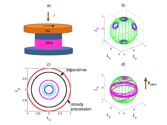
Figure 1: (Color online) The dynamics of AFM vector in the presence of spin-polarized current. a) AFM particle is placed between two electrodes, the top electrode being FM (polarizer). The spacer between FM and AFM is nonmagnetic to avoid the direct exchange coupling between the magnetic layers. b) Typical trajectories of $\mathbf{L}$ vector for circularly polarized modes. Different areas correspond to different equilibrium orientations (4 of 6 possible are shown). c) Projection of trajectories in $\mathbf{L}$ space to the $xy$ plane. Three inner circles correspond to the normal modes with different amplitudes in the vicinity of equilibrium state $\mathbf{L}\|z$. The last but one circle corresponds to separatrix and the outer circle is a steady state trajectory. d) Trajectory in the overcritical regime ($J=1.2J_{\mathrm{cr}}$). In the initial state $\mathbf{L}\|\mathbf{p}_{\mathrm{curr}}\|z$.

We consider a collinear AFM with two equivalent magnetic sublattices $\mathbf{M_{1}}$ and $\mathbf{M}_{2}$ and disregard a weak FM moment that can arise either from the intrinsic properties of material or from the surface effects. The coupling between the sublattices (characterized with a spin-flip field $H_{E}$) is much stronger than the external fields and the magnetic anisotropy. To this end, the AFM vector, $\mathbf{L}\equiv\mathbf{M_{1}}-\mathbf{M}_{2}$ of a fixed length $|\mathbf{L}|=2M_{0}$ unanimously describes the magnetic state of AFM nanoparticle. Corresponding dynamic equations for $\mathbf{L}$ are obtained within the standard Lagrange technique with the Lagrange function [26]

$$\mathcal{L}_{\mathrm{AFM}}=\frac{m_{L}}{2}\dot{\mathbf{L}}^{2}+\gamma m_{L}\left[\dot{\mathbf{L}}\cdot(\mathbf{L}\times\mathbf{H})\right]-w_{\mathrm{an}}(\mathbf{L})+\frac{\gamma^{2}m_{L}}{2}(\mathbf{L}\times{\mathbf{H}})^{2},$$ (2.1)

where $\mathbf{H}$ is an external magnetic field and $w_{\mathrm{an}}(\mathbf{L})$ is the energy of magnetic anisotropy that forms a potential well for AFM vector, $\gamma$ is the gyromagnetic ratio, $m_{L}$ is an effective mass related with the magnetic susceptibility.

The AFM layer has a cubic symmetry and magnetic anisotropy is modeled as follows:

$$w_{\rm an}=-\frac{H_{\mathrm{an}}}{8M_{0}^{3}}\left(L_{x}^{4}+L_{y}^{4}+L_{z}^{4}\right)\,,$$ (2.2)

where the orthogonal axes $x$, $y$ and $z$ coincide with the easy directions for the Néel vector, $H_{\mathrm{an}}\ll H_{E}$ is anisotropy field.

The Rayleigh dissipation function in the presence of spin-polarized current $J$ takes the form [7]:

$$\mathcal{R}_{\mathrm{AFM}}=\gamma_{\mathrm{AFM}}m_{L}\dot{\mathbf{L}}^{2}-\frac{\sigma J}{2\gamma M_{0}}\left[\mathbf{p}_{\mathrm{curr}}\cdot\left(\mathbf{L}\times\dot{\mathbf{L}}\right)\right].$$ (2.3)

Here, the first term models the internal damping with the coefficient $2\gamma_{\mathrm{AFM}}$ equal to AFMR linewidth, the constant $\sigma=\hbar\gamma\varepsilon/(2eM_{0}v_{\mathrm{AFM}})$ is proportional to the efficiency $\varepsilon$ of the spin transfer processes, $v_{\mathrm{AFM}}$ is the volume of AFM nanoparticle, $\hbar$ is the Plank constant, $e$ is the electron charge. Unit vector $\mathbf{p}_{\mathrm{curr}}$ is parallel to the spin current polarization.

Deterministic current-induced dynamics of AFM was analyzed in detail in reference [7]. Here we reproduce some characteristic features of this behaviour assuming that polarization of the spin current is parallel to an easy axis, $\mathbf{p}_{\mathrm{curr}}\|z$.

First, the critical current $J_{\mathrm{cr}}\equiv 2\gamma_{\mathrm{AFM}}\Omega_{\mathrm{AFMR}}/(\gamma\sigma H_{E})$ that separates the equilibrium and stationary regimes depends upon the AFMR frequency $\Omega_{\mathrm{AFMR}}\equiv\gamma\sqrt{H_{E}H_{\mathrm{an}}}$.

Second, in the subcritical regime, $|J|<J_{\mathrm{cr}}$, the AFM vector has three equilibrium orientations slightly deflected (due to STT) from $x$, $y$ and $z$ axes that define six (corresponding to $\mathbf{L}$ and $-\mathbf{L}$) basins of finite motion in the phase space. Typical phase trajectories in the vicinity of equilibrium points in nondissipative approximation correspond to the clockwise/counterclockwise rotations of AFM vector [circles in figure 1 (b)] and could be associated with the circular polarized normal modes with the frequencies $\pm\Omega_{\mathrm{AFMR}}$. Spin-polarized current acts as a negative damping for one of the modes (‘‘soft’’ mode) and as a positive damping for the other. The internal losses, however, suppress the negative damping and the real phase trajectories are the twisted spirals.

Third, in the overcritical regime ($|J|>J_{\mathrm{cr}}$), the stable non-equilibrium state occurs when the current-induced energy pumping exactly compensates the internal losses. AFM vector rotates in $xy$ plane (perpendicular to $\mathbf{p}_{\mathrm{curr}}$) with the current-dependent frequency $\omega=(J/J_{\mathrm{cr}})\Omega_{\mathrm{AFMR}}$ [the outer circle in figure 1 (c)]. The rotation direction coincides with that of the soft mode. This regime can be associated with the power generation.

Fourth, the motion of AFM vector shows two well separated time scales: fast rotation around $z$ axis with the frequency $\propto\Omega_{\mathrm{AFMR}}$ and slow, with the characteristic time $\propto 1/\gamma_{\mathrm{AFM}}$ variation of the polar angle from $0$ ($\mathbf{L}\|z$) to $\pi/2$ ($\mathbf{L}\perp z$). Figure 1 (d) shows an example of a typical trajectory with different time scales for the current-induced transition from the equilibrium state $\mathbf{L}\|z$ to the steady precession in $xy$ plane. Deviation from this scenario takes place only in the close vicinity of the separatrix [see figure 1 (c), next to the last circle] where the rotation frequency substantially diminishes.

Thus, in the vicinity of equilibrium and stationary steady states, the current-induced dynamics of AFM is characterized with a set of slow and fast variables and this can help to simplify the description of the stochastic behaviour.

3 Langevin dynamics and Fokker-Planck equations in energy representation

While only two variables in configuration space are enough to describe the dynamics of FM nanoparticle, the phase space of AFM nanoparticle includes at least four variables: generalized coordinates $\mathbf{L}$ and corresponding generalized momenta $\mathbf{P}_{L}$ (with account of normalization condition $|\mathbf{M}_{1}|=|\mathbf{M}_{2}|=M_{0}$ far below the Néel temperature). This results in rather complicated Langevin equations [23]:

$$\dot{\mathbf{L}} = \mathbf{P}_{L}/m_{L}-\gamma\mathbf{L}\times\mathbf{h}\,,$$

$$\dot{\mathbf{P}}_{L} = \mathbf{F}_{L}+\mathbf{F}_{\mathrm{diss}}-\gamma\left(\mathbf{P}_{L}-2\gamma_{\mathrm{AFM}}m_{L}\mathbf{L}\right)\times\mathbf{h}\,,$$ (3.1)

where $\mathbf{F}_{L}\equiv-\partial w_{\mathrm{an}}(\mathbf{L})/\partial\mathbf{L}$ is the potential (gradient) force, and the dissipative force $\mathbf{F}_{\mathrm{diss}}$ is expressed as follows:

$$\mathbf{F}_{\mathrm{diss}}\equiv-\left.\frac{\partial\mathcal{R}_{\rm AFM}}{\partial\dot{\mathbf{L}}}\right|_{\dot{\mathbf{L}}\rightarrow\mathbf{P}_{L}}=-2\gamma_{\mathrm{AFM}}\mathbf{P}_{L}-\frac{\sigma J}{2\gamma M_{0}}\mathbf{p}_{\mathrm{curr}}\times\mathbf{L}\,.$$ (3.2)

The random magnetic field $\mathbf{h}(t)$ in equation (3) models the white Gaussian noise with

$$\langle\mathbf{h}(t)\rangle=0,\qquad\langle h_{j}(t_{1})h_{k}(t_{2})\rangle=2D\delta_{jk}\delta(t_{1}-t_{2}),$$ (3.3)

where $2D$ represents the intensity of thermal fluctuations.

The above mentioned peculiarities of the current-induced dynamics make it possible to reduce the number of the effective phase variables in Langevin, (3), and corresponding Fokker-Planck equations. First, in the vicinity of equilibrium and stationary states, the motion of AFM vector is finite and can be decomposed to a linear combination of two independent (normal) modes shown in figure 2. Thus, one can use a set of canonically conjugated variables ‘‘action-angle’’, $I_{\pm},\varphi_{\pm}$ ($\pm$ correspond to the clock/counterclockwise rotations in configuration space), instead of coordinates and momenta. Second, in a low-temperature approximation, when the temperature $T$ is much less than the energy barrier between the different equilibrium/stationary states, all the essential phase trajectories for each mode are degenerated (have the same rotation/oscillation frequency, $\omega_{\pm}$). Thus, instead of action, one can use the energy of the mode, $E_{\pm}=I_{\pm}\omega_{\pm}$, as a canonical variable. Third, two time scales allow one to exclude the angle variables $\varphi_{\pm}$ by averaging over the period of rotation.

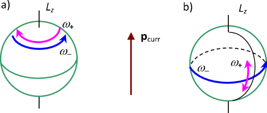
Figure 2: (Color online) Normal circularly polarized modes in the presence of spin-polarized current in a) subcritical and b) overcritical regimes. Typical trajectories lie over the sphere $|\mathbf{L}|=2M_{0}$ in configuration space.

As a result, Langevin equations (3) take the form:

$$\frac{\mathrm{d}E_{\pm}}{\mathrm{d}t}=-\overline{\mathbf{P}_{L}\cdot\mathbf{F}_{\mathrm{diss}}}+\gamma\left[\left(2\gamma_{\mathrm{AFM}}\mathbf{P}_{L}-\frac{\partial w_{\mathrm{an}}}{\partial\mathbf{L}}\right)\cdot\mathbf{L}\times\mathbf{h}\right],$$ (3.4)

where the overline means average over the period of rotation and the summands in r.h.s. of equation (3.4) should be expressed in terms of the average energies

$$E_{\pm}=\frac{\omega_{\pm}}{2\pi}\int_{0}^{2\pi/\omega_{\pm}}\left[\mathbf{P}_{L}^{2}/(2m_{L})+w_{\mathrm{an}}(\mathbf{L})\right]\mathrm{d}t.$$ (3.5)

An explicit closed form of the equation (3.5) will be obtained in next subsections in the limiting subcritical and overcritical regimes.

3.1 Subcritical regime $J<J_{\mathrm{cr}}$

Let us consider the basin of states in the vicinity of equilibrium point $\mathbf{L}\|\mathbf{p}_{\mathrm{curr}}\|z$ and choose $L_{x},L_{y}\ll 2M_{0}$ as generalized coordinates, $L_{z}\approx 2M_{0}$. Time dependence of the dynamic variables for the normal modes is given by the expressions

$$L_{x}+\mathrm{i}L_{y}=2M_{0}c_{\pm}\mathrm{e}^{\mathrm{i}\omega_{\pm}t},\qquad P_{Lx}+\mathrm{i}P_{Ly}=2\mathrm{i}M_{0}m_{L}\omega_{\pm}c_{\pm}\mathrm{e}^{\mathrm{i}\omega_{\pm}t},\qquad\omega_{\pm}=\pm\Omega_{\mathrm{AFMR}}\,.$$ (3.6)

The average energy is related with the amplitude $c_{\pm}$ as follows: $E_{\pm}=2E_{0}c_{\pm}^{2}$, where the value $E_{0}\equiv 2M^{2}_{0}\Omega_{\mathrm{AFMR}}^{2}m_{L}=M_{0}H_{\mathrm{an}}$ defines the characteristic energy scale for AFM nanoparticle.

Substituting expressions (3.6) into (3.2) and (3.4) we arrive at the system of two independent Langevin equations:

$$\frac{\mathrm{d}\varepsilon_{\pm}}{\mathrm{d}t} = {}-2\gamma_{\mathrm{AFM}}\left(1\pm\frac{J}{J_{\mathrm{cr}}}\right)\varepsilon_{\pm}+2\gamma\sqrt{\varepsilon_{\pm}}\left(\pm h_{x}\sin\Omega_{\mathrm{AFMR}}t-h_{y}\cos\Omega_{\mathrm{AFMR}}t\right)$$

$${}+\gamma\frac{2\gamma_{\mathrm{AFM}}}{\Omega_{\mathrm{AFMR}}}\left[2\sqrt{\varepsilon_{\pm}}\left(h_{x}\cos\Omega_{\mathrm{AFMR}}t\pm h_{y}\sin\Omega_{\mathrm{AFMR}}t\right)\mp\varepsilon_{\pm}h_{z}\right],$$

where $\varepsilon_{\pm}\equiv E_{\pm}/E_{0}$ is a dimensionless energy.

As it is seen from equation (3.1), the clock/counterclockwise modes [figure 2 (a)] interact with the current in different ways. If $J>0$, the effective damping of the first mode (with the energy $E_{+}$) increases and that of the second (with the energy $E_{-}$) decreases, due to the action of spin-polarized current.

Equations (3.1) are typical Langevin equations in energy representation considered in detail in [25]. The first summand in the r.h.s. describes the rate of direct energy exchange which depends upon the current value $J$. All but first summands in the r.h.s. of (3.1) account for system-environment interaction induced by the field fluctuations. The diffusion functions (coefficients before $h_{j}$) depend on energy and thus correspond to multiplicative noise. The last two terms (in square brackets) are multiplied by a small factor $\gamma_{\mathrm{AFM}}/\Omega_{\mathrm{AFMR}}\ll 1$ and thus can be neglected.

In the accepted approximation of noninteracting modes, the distribution function in phase space, $f(\mathbf{L},\mathbf{P}_{L};t)$, can be factorized as follows: $f(\mathbf{L},\mathbf{P}_{L};t)\Rightarrow f_{+}(E_{+};t)f_{-}(E_{-};t)$. The Fokker-Planck equations for $f_{\pm}$ are deduced in a standard manner from (3.1) in Stratonovich convention and take the form:

$$\frac{\partial f_{\pm}(E_{\pm})}{\partial t}=\frac{\partial}{\partial E_{\pm}}\left\{\left[\gamma^{2}DE_{0}\sqrt{E_{\pm}}\frac{\partial}{\partial E_{\pm}}\sqrt{E_{\pm}}+2\gamma_{\mathrm{AFM}}\left(1\pm\frac{J}{J_{\mathrm{cr}}}\right)E_{\pm}\right]f_{\pm}(E_{\pm})\right\}.$$ (3.8)

From the stationary solution of (3.8) one gets the AFM probability distribution function $f(E_{+},E_{-})=f_{+}(E_{+})f_{-}(E_{-})\sqrt{E_{+}E_{-}}$ (with due account of Jacobian):

$$f(E_{+},E_{-})=f_{0}\exp{\left\{-\frac{2\gamma_{\mathrm{AFM}}}{\gamma^{2}DE_{0}}\left[\left(1+\frac{J}{J_{\mathrm{cr}}}\right)E_{+}+\left(1-\frac{J}{J_{\mathrm{cr}}}\right)E_{-}\right]\right\}},$$ (3.9)

where $f_{0}$ is a normalization constant and the diffusion coefficient is related with the temperature $T$ through the fluctuation-dissipation theorem as follows:

$$D=\frac{2\gamma_{\mathrm{AFM}}}{\gamma^{2}E_{0}}T.$$ (3.10)

3.2 Overcritical regime $J>J_{\mathrm{cr}}$

In the overcritical regime, the motion can be decomposed (like it was done in the reference [27] for FM) into steady rotation of AFM vector in $xy$ plane with the frequency $\omega_{-}$ and small meridian oscillations of $\mathbf{L}$ vector with the frequency $\omega_{+}$ [see figure 2 (b)].

The ‘‘$+$’’-mode is parametrized as follows:

$$L_{z}\ =c\mathrm{e}^{\mathrm{i}\omega_{+}t},\qquad\qquad\qquad\quad P_{Lz}=2\mathrm{i}M_{0}m_{L}\omega_{+}c\mathrm{e}^{\mathrm{i}\omega_{+}t},$$ (3.11)

$$\omega_{+}=\Omega_{\mathrm{AFMR}}\sqrt{\frac{3}{4}+\frac{J^{2}}{J^{2}_{\mathrm{cr}}}},\ \,\qquad E_{+}=2E_{0}\left(\frac{3}{4}+\frac{J^{2}}{J^{2}_{\mathrm{cr}}}\right)c^{2}.$$

The corresponding Langevin and Fokker-Planck equations are analogous to (3.1) and (3.8).

Parametrization of ‘‘$-$’’-mode coincides with that in equation (3.6) with $c_{-}=1$. In this particular case, the proper dynamic variable is action $I_{-}=8\pi M_{0}^{2}m_{L}\omega_{-}$. The corresponding Langevin equation takes the form

$$\frac{\mathrm{d}I_{-}}{\mathrm{d}t}=-2\gamma_{\mathrm{AFM}}\left(I_{-}-8\pi M_{0}^{2}m_{L}\omega_{-}^{(0)}\right)-\gamma I_{-}h_{z}\,,$$ (3.12)

where $\omega_{-}^{(0)}=-(J/J_{\mathrm{cr}})\Omega_{\mathrm{AFMR}}$ is the frequency of steady rotation. Substituting $I_{-}=4\pi M_{0}\sqrt{2m_{L}E_{-}}$ into (3.12) we get Langevin equation in energy representation:

$$\frac{\mathrm{d}E_{-}}{\mathrm{d}t}=-4\gamma_{\mathrm{AFM}}\left(E_{-}-\frac{J}{J_{\mathrm{cr}}}\sqrt{E_{0}E_{-}}\right)-2\gamma E_{-}h_{z}\,.$$ (3.13)

The corresponding Fokker-Planck equation is deduced as follows:

$$\frac{\partial f_{-}(E_{-})}{\partial t}=\frac{\partial}{\partial E_{-}}\left\{\left[4\gamma^{2}DE_{-}\frac{\partial}{\partial E_{-}}E_{-}+4\gamma_{\mathrm{AFM}}\left(E_{-}-\frac{J}{J_{\mathrm{cr}}}\sqrt{E_{0}E_{-}}\right)\right]f_{-}(E_{-})\right\}.$$ (3.14)

Ultimately, the stationary AFM distribution function in the overcritial regime takes the form:

$$f(E_{+},E_{-})=f_{0}\exp{\left\{-\frac{4E_{+}}{\left[3+4\left(J/J_{\mathrm{cr}}\right)^{2}\right]T}-\frac{\left(E_{-}-E_{0}J^{2}/J^{2}_{\mathrm{cr}}\right)^{2}}{2TE_{0}J^{2}/J^{2}_{\mathrm{cr}}}\right\}},$$ (3.15)

where we have taken into account the relation (3.10) and assumed that $T\ll E_{0}$.

4 Discussion

In the previous section we derived the stochastic equations for the current-controlled AFM nanoparticle in the low temperature approximation, $T\ll E_{0}$. So, the magnetic anisotropy energy $E_{0}$ sets the energy scale of the system and limits the validity of equations (3.15). AFMs with high Néel temperature show a characteristic density of magnetic anisotropy $10^{3}\div 10^{4}$ J/m³ (see, e.g. [28] for Mn₈₂Ni₁₈). So, $E_{0}\propto 10^{-20}\div 10^{-19}$ J for the nanoparticles with the typical size $50\times 50\times 5$ nm³. Thus, the proposed model can be applied up to the room temperature, $T_{\mathrm{RT}}=4\cdot 10^{-21}$ J.

Neglecting the swap processes between different basins, we found two stationary solutions of Fokker-Planck equations: in the vicinity of equilibrium, (3.9), and nonequilibrium steady (3.15) states.

For the noncritical (‘‘$+$’’) mode, the probability function $f(E_{+})$ [see (3.9) and (3.15)] follows the Boltzmann law with the current-dependent effective temperature

$$T_{\mathrm{eff}}^{(+)}=T\left\{\begin{array}[]{cc}\left(1+J/J_{\mathrm{cr}}\right)^{-1}\,,&\qquad J<J_{\mathrm{cr}}\,,\\ 0.75+J^{2}/J^{2}_{\mathrm{cr}}\,,&\qquad J>J_{\mathrm{cr}}\,.\end{array}\right.$$ (4.1)

In the subcritical regime ($J<J_{\mathrm{cr}}$), the ‘‘soft’’ (‘‘$-$’’) mode shows the Boltzmann-like distribution which changes to the Gauissian-like with the current-dependent average, $E_{-}^{(0)}\equiv E_{0}J^{2}/J^{2}_{\mathrm{cr}}$, and current-dependent dispersion, $TE_{0}J^{2}/J^{2}_{\mathrm{crit}}$ at $J>J_{\mathrm{cr}}$. In the subcritical region, the effective temperature $T_{\mathrm{eff}}^{(-)}=T/(1-J/J_{\mathrm{cr}})$ diverges as $J\rightarrow J_{\mathrm{cr}}-0$. This singularity can be avoided with due account of the swap processes [see the trajectory in figure 1 (d)] that are important in the vicinity of critical current $J\approx J_{\mathrm{cr}}$. This problem is, however, out of scope of this paper.

The statistical properties of the ‘‘soft’’ mode in AFM and FM nanoparticles in the presence of spin-polarized current are similar: Boltzmann-like distribution and critical behaviour of the effective temperature in subcritical region, and Gaussian-like distribution in overcritical regime [13]. The current dependencies of average energy and dispersion are, however, different, as will be discussed below.

Figure 3 shows the distribution function, $f(E)$, that depends on the total magnetic energy $E=E_{+}+E_{-}$ of AFM nanoparticle. Dependencies $f(E)$ for different current values are calculated from (3.9) and (3.15) as conventional probabilities.

In the subcritical regime ($J/J_{\mathrm{cr}}=0.1,0.5,0.9$), the distribution function is asymmetric with maximum at

$$E_{\mathrm{max}}=\frac{T}{J/J_{\mathrm{cr}}}\tanh^{-1}\frac{J}{J_{\mathrm{cr}}}\approx T.$$ (4.2)

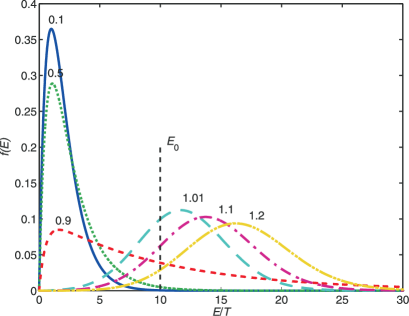
Figure 3: (Color online) Energy distribution function for different current values $J/J_{\mathrm{cr}}$ (shown with numbers near the curves) in the subcritical ($J<J_{\mathrm{cr}}$) and overcritical ($J>J_{\mathrm{cr}}$) regimes. Energy is measured in the dimensionless units, $E/T$. Vertical dashed line shows the energy $E_{0}=10T$ in the overcritical regime.

Average magnetic energy of nanoparticle, $E_{\mathrm{av}}\equiv\langle E\rangle=T_{\mathrm{eff}}^{(+)}+T_{\mathrm{eff}}^{(-)}$, consists of the noisy component only and diverges as $J\rightarrow J_{\mathrm{cr}}$. Energy fluctuation,

$$\Delta E\equiv\sqrt{\langle\left(E-E_{\mathrm{av}}\right)^{2}\rangle}=\left(T_{\mathrm{eff}}^{(+)}+T_{\mathrm{eff}}^{(-)}\right)\sqrt{\frac{1}{2}\left(1+\frac{J^{2}}{J^{2}_{\mathrm{cr}}}\right)}$$ (4.3)

diverges in the same way [see figure 4 (a)]. Thus, the quality factor, $Q_{\mathrm{AFM}}=E_{\mathrm{av}}/\Delta E$ diminishes down to 1 as $J\rightarrow J_{\mathrm{cr}}-0$. This tendency is quite obvious if one takes into account the noisy source of the energy in a system. The singularity in $\Delta E$ emphasizes the role of thermal noise in the transition from equilibrium to nonequilibrium steady state in the vicinity of critical current.

In the overcritical regime ($J/J_{\mathrm{cr}}=1.01,\,1.1,\,1.2$), the distribution function $f(E)$ has a Gaussian-like shape with the maximum close to the average energy $E_{\mathrm{av}}$. Both $E_{\mathrm{av}}$ and $\Delta E$ grow with current [see figure 4 (b)]. However, the main contribution into $E_{\mathrm{av}}$ arises from the deterministic (low entropy) current-induced rotation of AFM vector, while $\Delta E$ originates from the noise slightly intensified by the current. Thus, the quality factor $Q_{\mathrm{AFM}}$ is finite at $J=J_{\mathrm{cr}}$ and increases with current almost linearly [inset in figure 4 (b)]. By contrast, the quality factor for FM nanoparticle, $Q_{\mathrm{FM}}\propto\sqrt{1-J_{\mathrm{cr}}/J}$, vanishes in the close vicinity of $J_{\mathrm{cr}}$ in the supercritical regime. This opens up the way for potential applications of AFM nanoparticles as active elements of spintronic devices and as a possible alternative to FM nanooscillators. The model, however, should be further developed to account for the Joule heating, current fluctuations, etc.

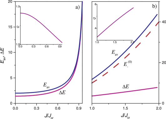
Figure 4: (Color online) Current dependence of the average energy, $E_{\mathrm{av}}$, and energy fluctuation, $\Delta E$ in a) subcritical ($J<J_{\mathrm{cr}}$) and b) overcritical ($J>J_{\mathrm{cr}}$) regimes. Insets show the current dependence of the quality factor, $Q_{\mathrm{AFM}}=E_{\mathrm{av}}/\Delta E$. The energy $E_{0}=10T$. Dashed line shows the current-dependence of the ‘‘soft’’ mode energy $E_{-}^{(0)}=E_{0}J^{2}/J_{\mathrm{cr}}^{2}$ .

In summary, we considered the current-induced dynamics of AFM nanoparticle in the presence of white Gaussian noise which originates from the random magnetic fields. We found the stationary energy distribution functions in two regimes: subcritical, when the spin-polarized current is too small to reorient AFM vector from the initial equilibrium state, and overcritical, when the spin-polarized current keeps steady rotation of AFM vector. Average energy and energy fluctuations in the subcritical regime show the critical behaviour as $J\rightarrow J_{\mathrm{cr}}$. This can be used to facilitate the current-induced reorientation of AFM vector. In the overcritical regime, the quality factor of AFM particle as nanooscillator can be increased by adjusting the current value.

Ukrainian 0

Антиферомагнiтний наноосцилятор зi спiновим крутильним моментом в присутностi магнiтних шумiв О.В. Гомонай${}^{\textsf{\footnotesize{\mbox{?},\penalty 1000\mbox{?}}}}$, В.М. Локтєв${}^{\textsf{\footnotesize{\mbox{?}}}}$

             
${}^{\textsf{\footnotesize 1}}$ Нацiональний технiчний унiверситет України ‘‘КПI’’, пр. Перемоги, 37, 03056 Київ, Україна ${}^{\textsf{\footnotesize 2}}$ Iнститут теоретичної фiзики iм. М.М. Боголюбова НАН України,
вул. Метрологiчна, 14-б, 03680 Київ, Україна

References

- [1] Slonczewski J., J. Magn. Magn. Mater., 1996, 159, L1; doi:10.1016/0304-8853(96)00062-5.
- [2] Berger L., Phys. Rev. B, 1996, 54, No. 13, 9353; doi:10.1103/PhysRevB.54.9353.
- [3] Kiselev S.I., Sankey J.C., Krivorotov I.N., Emley N.C., Schoelkopf R.J., Buhrman R.A., Ralph D.C., Nature, 2003, 425, 380; doi:10.1038/nature01967.
- [4] Tulapurkar A.A., Suzuki Y., Fukushima A., Kubota H., Maehara H., Tsunekawa K., Djayaprawira D.D., Watanabe N., Yuasa S., Nature, 2005, 438, No. 11, 339; doi:10.1038/nature04207.
- [5] Gerhart G., Bankowski E., Melkov G.A., Tiberkevich V.S., Slavin A.N., Phys. Rev. B, 2007, 76, No. 2, 024437; doi:10.1103/PhysRevB.76.024437.
- [6] Yamaguchi A., Motoi K., Hirohata A., Miyajima H., Miyashita Y., Sanada Y., Phys. Rev. B, 2008, 78, No. 10, 104401; doi:10.1103/PhysRevB.78.104401.
- [7] Gomonay H.V., Loktev V.M., Phys. Rev. B, 2010, 81, No. 14, 144427; doi:10.1103/PhysRevB.81.144427.
- [8] Linder J., Phys. Rev. B, 2011, 84, No. 9, 094404; doi:10.1103/PhysRevB.84.094404.
-
[9]
Rippard W.H., Pufall M.R., Kaka S., Russek S.E., Silva T.J., Phys. Rev. Lett.,
2004, 92, No. 2, 027201;
doi:10.1103/PhysRevLett.92.027201. - [10] Deac A.M., Fukushima A., Kubota H., Maehara H., Suzukia Y., Yuasa S., Nagamine Y., Tsunekawa K., Djayaprawira D.D., Watanabe N., Nat. Phys., 2008, 4, 803; doi:10.1038/nphys1036.
- [11] Brown W.F., Phys. Rev., 1963, 130, 1677; doi:10.1103/PhysRev.130.1677.
- [12] Apalkov D.M., Visscher P.B., Phys. Rev. B, 2005, 72, 180405; doi:10.1103/PhysRevB.72.180405.
- [13] Tiberkevich V., Slavin A., Kim J.V., Appl. Phys. Lett., 2007, 91, No. 19, 192506; doi:10.1063/1.2812546.
-
[14]
Swiebodzinski J., Chudnovskiy A., Dunn T., Kamenev A., Phys. Rev. B, 2010,
82, 144404;
doi:10.1103/PhysRevB.82.144404. - [15] Dunn T., Kamenev A., Appl. Phys. Lett., 2011, 98, No. 14, 143109; doi:10.1063/1.3576929.
- [16] Prokopenko O., Melkov G., Bankowski E., Meitzler T., Tiberkevich V., Slavin A., Appl. Phys. Lett., 2011, 99, No. 3, 032507; doi:10.1063/1.3612917.
- [17] Raikher Y.L., Stepanov V.I., J. Exp. Theor. Phys., 2008, 107, No. 3, 435; doi:10.1134/S1063776108090112 [Zh. Eksp. Teor. Fiz., 2008, 134, No. 3, 514 (in Russian)].
- [18] Ouari B., Kalmykov Y.P., Phys. Rev. B, 2011, 83, 064406; doi:10.1103/PhysRevB.83.064406.
- [19] Mishra S.K., Eur. Phys. J. B, 2010, 78, 65; doi:10.1140/epjb/e2010-00293-0.
- [20] Mishra S.K., Subrahmanyam V., Phys. Rev. B, 2011, 84, No. 2, 024429; doi:10.1103/PhysRevB.84.024429.
- [21] Borovik-Romanov A.S., Rudashevskii E.G., Turov E.A., Shavrov V.G., Sov. Phys. Uspekhi, 1984, 27, No. 8, 642; doi:10.1070/PU1984v027n08ABEH004078.
- [22] Akhiezer A.I., Bar’yakhtar V.G., Peletminskii S.V., Spin Waves, North-Holland Series in Low Temperature Physics, vol. 1, North-Holland, Amsterdam, 1968.
- [23] Gomonay H.V., Loktev V.M., Eur. Phys. J. ST, 2013 (in press); Preprint arXiv:1207.1997, 2012.
- [24] Dunn T., Chudnovskiy A.L., Kamenev A., Preprint arXiv:1110.3750, 2011.
- [25] Lev B.I., Kiselev A.D., Phys. Rev. E, 2010, 82, No. 3, 031101; doi:10.1103/PhysRevE.82.031101.
- [26] Bar’yakhtar I., Ivanov B., Fiz. Nizk. Temp., 1979, 5, 361 (in Russian).
-
[27]
Denisov S.I., Lyutyy T.V., Hänggi P., Trohidou K.N., Phys. Rev. B, 2006,
74, 104406;
doi:10.1103/PhysRevB.74.104406. - [28] Takahashi M., Tsunoda M., J. Phys. D: Appl. Phys., 2002, 35, No. 19, 2365; doi:10.1088/0022-3727/35/19/307.
Ukrainian \adddialect\l@ukrainian0 \l@ukrainian