Luneburg lens waveguide networks

Abstract

We investigate certain configurations of Luneburg lenses that form light propagating and guiding networks. We study single Luneburg lens dynamics and apply the single lens ray tracing solution to various arrangements of multiple lenses. The wave propagating features of the Luneburg lens networks are also verified through direct numerical solutions of Maxwell’s equations. We find that Luneburg lenses may form efficient waveguides for light propagation and guiding. The additional presence of nonlinearity improves the focusing characteristics of the networks.

Keywords : Metamaterials, gradient index lenses, Luneburg lens, Lagrangian optics, Hamiltonian ray-tracing, waveguides, Kerr effect.

1 Introduction

Gradient Index (GRIN) metamaterials are formed through spatial variation of the index of refraction and lead to enhanced light manipulation in a variety of circumstances. These metamaterials provide natural means for constructing various types of waveguides and other optical configurations that guide and focus light in specific desired paths. Different configurations have been tested experimentally while the typical theoretical approach uses Transformation Optics (TO) methods to cast the original inhomogeneous index problem to an equivalent one in a deformed space [1, 2, 3, 4, 5, 6]. While this approach is mathematically elegant, it occasionally hides the intuition obtained through more direct means. Furthermore, a general, continuous GRIN waveguide may be hard to analyze in more elemental units and relate its global features to these units. In the present work, we adopt precisely this latter avenue, viz. attempt to construct waveguide structures that are seen as lattices, or networks, of units with specific features. This is a ”metamaterials approach”, where specific properties of the ”atomistic” units are inherited as well as expanded in the network.

The ”atomic” unit of the network is a Luneburg lens (LL); the later is a spherical construction where the index or refraction varies from one, in its outer boundary, to $\sqrt{2}$ in the center with a specific functional dependence on the lens radius [7, 8]. Its basic property, in the geometrical optics limit, is to focus parallel rays on the spherical surface on the opposite side of the lens [6, 7, 8, 9, 10, 11, 12, 13, 14]. This feature makes LL’s quite interesting for applications since the focal surface is predefined for parallel rays of any initial angle. While the rays traverse the lens, they suffer variable deflections depending on their distance from the optical axis ray, leading to a point image on the lens surface. This property of the spherical LL is also shared by its cylindrical equivalent formed by long dielectric cylinders while the light wave-vector impinges perpendicularly to the cylindrical axis. This geometry turns the problem into a two dimensional one, constructed for any plane that cuts the LL cylinder perpendicular to its axis. The work in this article focuses on exactly this type of cylindrical LLs and, as a result, our approach is strictly two dimensional [7, 8, 10].

In the present work we analyze the ray trajectories in a single LL and subsequently we use this analysis in waveguides build exclusively through LLs. Specifically, in the next section we present analytical approaches for the trajectories traversing a LL [1, 2, 3, 7, 8, 10, 15, 16, 17, 18, 19] and derive explicitly a solution expressing the ordinate of the trajectory as a function of the abscissa in Cartesian coordinates. In section 3 we introduce the main point of the present work, viz. the formation of Luneburg Lens Waveguides (LLW) through the arrangement of multiple LLs [13] in geometrically linear or bent configurations. The LLWs are investigated through dynamical maps stemming from the analytical solution for the single LL. In section 4 we investigate the same LLWs but using a direct solution of Maxwell’s equations and find compatibility with the results of ray tracing approach of the previous section. Additionally, we also use nonlinearity in the index of refraction and find better focusing characteristics [12, 20]. Finally, in section 5 we conclude.

2 Single Luneburg lens

2.1 Ray tracing solution

The general problem we have at hand is light propagation in an inhomogeneous isotropic medium with an index of refraction $n(\vec{r})$, where $\vec{r}$ is the position vector. Although this problem has been tackled though various approaches, for the purposes of our problem we need the exact solution for propagation through a single LL, which is itself an inhomogeneous medium. What we need is a ray tracing solution for a single LL that, in turn, will be used for providing the basic element in a map approach for the ray dynamics in LL networks.

Given the recent interest in LLs we present below three ways for obtaining the ray tracing solution for the single LL; these explicit solutions from the different approaches may be useful in other LL studies as well. The first two methods (section 2.2 and Appendix A.1 respectively) are based on the Fermat principle for optical path or travel time minimization [1, 7, 15, 16, 17, 18] while the last one (Appendix A.2) uses a geometrical optics approach to Helmholtz wave equation [1, 7, 17, 18, 19, 23]. In all cases we focus on the specific, cylindrically symmetric, LL index of refraction $n(\vec{r})$  [7, 8, 10, 19]

$$n(r)=\sqrt{2-(\frac{r}{R})^{2}}$$ (1)

where $R$ is the radius of the lens while $r$ is the radial distance from the center in the interior of the lens, i.e. $r\leqslant R$. The LL is supposed to be embedded in a medium with index equal to one, leading to a continuous change in the index variation as a ray enters the lens.

2.2 Quasi 2D ray solution

The optical path length $\mathcal{S}$ of a ray from a point A to B is given by [1, 7, 15, 16, 17, 18]

$$\mathcal{S}=\int_{A}^{B}nds$$ (2)

In polar coordinates the arc length is $ds=\sqrt{1+r^{2}\dot{\phi}^{2}}dr$, with $\dot{\phi}\equiv d\phi/dr$ where the coordinate $r$ is considered a ”generalized time”. As a result Fermat’s variational integral of Eq. (2), becomes

$$\mathcal{S}=\int_{A}^{B}n(r)\sqrt{1+r^{2}\dot{\phi}^{2}}dr$$ (3)

and leads to the Optical Lagrangian [1, 15, 16]

$$\mathcal{L}(\phi,\dot{\phi},r)=n(r)\sqrt{1+r^{2}\dot{\phi}^{2}}$$ (4)

The shortest optical path is obtained through minimization of the integral of Eq. (3) and may be found through the solution of the Euler-Lagrange equation for the Lagrangian of Eq. (4), viz.

$$\frac{d}{dr}\frac{\partial\mathcal{L}}{\partial\dot{\phi}}=\frac{\partial\mathcal{L}}{\partial\phi}$$ (5)

Since the Lagrangian (4) is cyclic in $\phi$, we have $\partial\mathcal{L}/\partial\phi=0$ and thus $\partial\mathcal{L}/\partial\dot{\phi}=\mathcal{C}$ where $\mathcal{C}$ is a constant. We thus obtain for the Lagrangian of Eq. (4) [1, 15, 16]

$$\frac{n(r)r^{2}}{\sqrt{1+r^{2}\dot{\phi}^{2}}}\dot{\phi}=\mathcal{C}$$ (6)

This is a nonlinear differential equation describing the trajectory $r(\phi)$ of a ray in the interior of LL. Replacing the term $\dot{\phi}\equiv d\phi/dr$ and solving for $d\phi$, we obtain a first integral of motion, i.e.

$$\int{d\phi}=\int{\frac{\mathcal{C}}{r\sqrt{n^{2}r^{2}-\mathcal{C}^{2}}}dr}$$ (7)

The expression of Eq. (7) holds for arbitrary index functions $n(r)$. Using the specific LL refractive index function of Eq. (1) we evaluate the integral (7) and obtain the ray tracing equation for a single LL as follows

$$r(\phi)=\frac{\mathcal{C^{\prime}}R}{\sqrt{1-\sqrt{1-\mathcal{C^{\prime}}^{2}}~{}\sin(2(\phi+\beta))}}$$ (8)

where $\mathcal{C^{\prime}}$ and $\beta$ are constants. This analytical expression may be cast in a direct Cartesian form for the $(x,y)$ coordinates of the ray; after some algebra we obtain

$$(1-T\sin(2\beta))x^{2}+(1+T\sin(2\beta))y^{2}$$

$$-2T\cos(2\beta)xy+(T^{2}-1)R^{2}=0$$ (9)

where $T$ and $\beta$ are constants. We note that Eq. (2.2) is an equation for an ellipse. This result agrees with the Luneburg theory and states that inside a LL light follows elliptic orbits.

The constants $T$ and $\beta$ of Eq. (2.2) are determined through the ray boundary (or ”initial” conditions) and depend on the initial propagation angle $\theta$ of a ray that enters the lens at the point $(x_{0},y_{0})$ lying on the circle at the lens radius $R$ [15]. The entry point of the ray is at $(x,y)=R(\cos(\theta+\pi),\sin(\theta+\pi))=-R(\cos\theta,\sin\theta)$. Substituting these expressions in Eq. (2.2) we obtain after some algebra

$$T=\sin(2\beta+2\theta)$$ (10)

In order to determine both constants $T,\beta$ we need an additional relation connecting them. Taking the derivative of the Eq.(2.2) respect to $x$ and regarding the fact that $dy/dx=\tan(\theta)$, where $\theta$ the initial propagation angle. In addition, using the labels $(x_{0},y_{0})$ for the initial ray point on the LL surface, we set $x=x_{0}$ and $y=y_{0}$ in Eq.(2.2) we solve for $T$ and obtain

$$T=\frac{x_{0}+y_{0}\tan(\theta)}{\tan(\theta)[x_{0}\cos(2\beta)-y_{0}\sin(2\beta)]+[x_{0}\sin(2\beta)+y_{0}\cos(2\beta)]}$$ (11)

The Eqns. (10) and (11) consist of an algebraic nonlinear system expressing the constants $T$ and $\beta$ as a function of the initial ray entry point in the LL at $(x_{0},y_{0})$ with angle $\theta$. Combining the Eqns. (10), (11) and after simplifications we obtain

$$\beta=\frac{1}{2}(\tan^{-1}({x_{0}}/{y_{0}})-\theta)$$ (12)

therefore, according Eq. (10)

$$T=\sin(\tan^{-1}(x_{0}/y_{0})+\theta)$$ (13)

Substituting now the Eqs.(12,13) to Eq.(2.2) and solving for $y$, we obtain the equation

$$y(x)=\frac{(2x_{0}y_{0}+R^{2}\sin(2\theta))}{2x_{0}^{2}+(1+\cos(2\theta))R^{2}}x~{}~{}+$$

$$+\frac{\sqrt{2}Ry_{0}\cos(\theta)\sqrt{(1+\cos(2\theta))R^{2}+2x_{0}^{2}-2x^{2}}}{2x_{0}^{2}+(1+\cos(2\theta))R^{2}}-$$

$$-\frac{x_{0}\sin(\theta)\sqrt{(1+\cos(2\theta))R^{2}+2x_{0}^{2}-2x^{2}}}{2x_{0}^{2}+(1+\cos(2\theta))R^{2}}~{}~{}~{}~{}~{}$$ (14)

where $x_{0},y_{0}$ give the initial ray entry point and $\theta$ the initial propagation angle.

The Eq. (2.2) describes the complete solution of the ray trajectory through a LL; in the simplest case where all rays are parallel to the $x$ axis, the initial angle $\theta=0$ and Eq. (2.2) simplifies to

$$y(x)=\frac{y_{0}}{x_{0}^{2}+R^{2}}(x_{0}x+R\sqrt{R^{2}+x_{0}^{2}-x^{2}})$$ (15)

We note that in order to determine the exit angle $\theta^{\prime}$, i.e. the angle with which each ray exits the lens, we may take the arc tangent of the derivative of Eq. (2.2) wrt $x$ at the focal point on the surface of lens at $x=R\cos(\theta)$. The solution of Eq. (2.2) may be used to study several configurations of LLs; however special provisions are necessary in cases where the rays need to turn backwards. It is thus more practical to use parametric solutions where the ray coordinates $x,y$ are both dependent variables. This approach is explained in the Appendix where the parametric solution of Eq. (43) is derived.

3 Luneburg Lens Waveguides

The analytical solutions for the single LL trajectory, viz. Eqs.(2.2) or (43) may be used in order to study analytically the ray transfer through various configurations of LLs that form waveguides [13]. Using the initial entry point on the LL $(x_{0},y_{0})$ as well as the initial ray angle $\theta$ we obtain through Eq. (2.2) the exit point $(x,y)$ and the associated exit angle $\theta^{\prime}$. We may thus form a mapping from $(x_{0},y_{0},\theta)$ to $(x,y,\theta^{\prime})$; further propagation in the surrounding medium is rectilinear while the entry to the next LL is governed by a new initial entry point with angle equal to the previous exit angle. The resulting ray may be traced easily through the map.

A geometrically linear arrangement of touching LLs on a straight line is shown in in Fig. 1; this configuration forms a waveguide that channels the light through. Depending on the number of lenses even or odd number) the rays focus in the last LL surface or exit as they entered respectively. In both cases we sent a beam of rays parallel to the axis of symmetry of the network.

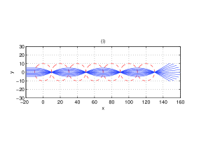
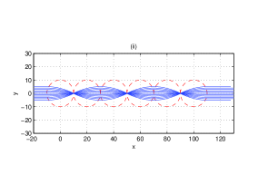
Figure 1: The red dotted lines denote the arrangement of lenses. The blue lines show the ray tracing. Light is guided by Luneburg lenses across the linear network. (i) Arrangement with 7 lenses (left figure). We can see that all rays are focus on the last lens. (ii) Arrangement with 6 lenses (right figure). All rays exit in the same mode as originally entered, i.e. parallel to the waveguide axis.

In Fig. (2) we use the ray tracing equations, Eqs.(2.2) or (43) to study the propagation along curved arrangements of LL’s. We observe the efficient channeling of the rays through the network that leads to a complete ray banding at a right angle. Some rays escape in the sharp bend, but generally the guiding is very efficient for such a drastic change of direction.

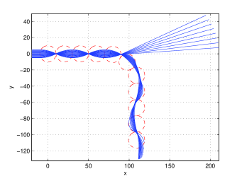
Figure 2: A right angle waveguide is formed through a network of eleven Luneburg lenses. The ray-tracing is performed analytically using Eq. (43). We observe efficient guiding with a total bend of $90^{o}$ degrees.

In Fig. (3) we form a full circle bend waveguide through a sequence of LLs and follow the light propagation in the geometric optics limit. We find that light may propagate efficiently through a loop, signifying that arbitrary waveguide formation and guiding is possible.

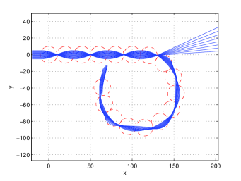
Figure 3: A full circle bend waveguide formed through seventeen Luneburg lenses. The ray-tracing is performed through the ray tracing methods. We see that Luneburg waveguides can guide light in a complete circle bend trajectory; more complex paths are also possible.

The LL network cases presented (linear, right angle, curved) signify that LLs may be used as efficient waveguides. Their advantage over usual dielectric guides is that light bending occurs naturally through the LL properties while the outgoing light may be also focused, if so desired. In bends there are naturally some losses that, in the geometric optics limit, may be estimated by comparing the number of the incoming to the outgoing rays, viz. $N_{IN}$) versus $N_{OUT}$ respectively. In the linear arrangement of waveguides, as in Fig. 1, the performance is perfect since $N_{IN}=N_{OUT}$. In the bend cases, such as in the right angle arrangement of Fig. 2 as well as in the full circle bend waveguide of Fig. 3, we find $N_{OUT}/N_{IN}=13/21=0.6$. We note that the aforementioned losses depend also on the ray coverage of the initial lens as well as the sharpness of the bend; the losses can be reduced by manipulating appropriately these two factors.

4 Wave propagation in Luneburg lens networks

4.1 Propagation through LL waveguides

In the present section we present results for the true wave propagation in networks of LLs. The simulations we done both with a homemade FDTD based algorithm that was tested against COMSOL Multiphysics^® software. Both gave good agreement and, as a result, we show only the results obtained from the latter. In order to be more realistic, we used Gaussian beams instead of plane waves [12, 20]. In the single LL case the effect of the gaussian beam shape is to shift the focus outside the LL surface, an effect that may be compensated though nonlinearity  [12, 20]. Specifically, we simulate all three arrangements shown previously, viz. Figs. 1, 2 and 3 and we calculate numerically the losses of the guiding. Subsequently, we introduce nonlinearity and show that the Kerr effect improves guiding as well as focusing of the beam through Luneburg waveguide.

In order to setup our arrangements we use silica glass for the Luneburg lenses with refractive index variation as in Eq.(1). In addition we use air for the outer medium with index of refraction $n=1$ [11, 12, 14, 6] with a monochromatic TM mode Gaussian EM wave. We perform all simulations in microwave regime with wavelength $\lambda=1cm$. In all simulations the radius of each LL is ten times greater that the wavelength, i.e. $R=10\lambda=10cm$. Finally, in the lattice edge we apply PML boundary conditions [21].

In Figs. (4-7) we show the results for the full propagation of EM waves through LLs waveguides. We plot the steady state of the absolute value of the electric field.

For the linear arrangement of LL waveguides we study a sequence with seven and six lenses, Figs. 4 and 5 respectively. In the case with even number of lenses, as in Fig. 4, the ray beam is guided and defocusses while exciting the waveguide. On the other hand, in the case with odd number of lenses, as in Fig. 5, the beam focuses in the last lens. The results obtained are compatible with those obtained through the ray tracing methods of Fig. 1 The right angle bend is shown in Fig. 6, while in Fig. 7 we have a full circle arrangement of LLs; these arrangements are the same as those analyzed in Fig. 2 and Fig. 3 respectively. In all cases studied, the numerical solution of Maxwell’s equations is compatible with the findings obtained through the ray tracing map.

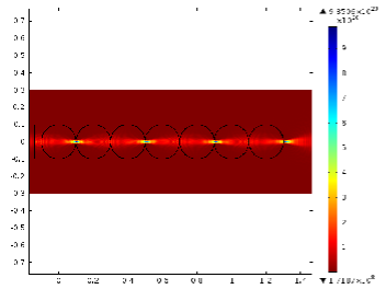
Figure 4: Linear Luneburg waveguide arrangement with seven lenses. Beam guiding and focusing on the surface of the last lens is observed. The result is in agreement with Fig. 1(i). Furthermore, no losses are observed.

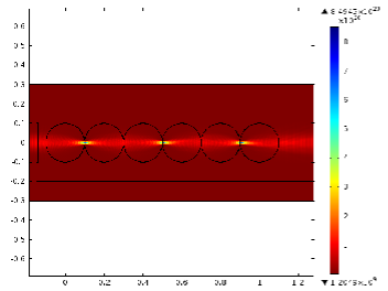
Figure 5: Linear waveguide arrangement formed with six Luneburg lenses. The EM wave is guided through the linear network of lenses and the wave defocusses in the last lens. The result is in agreement with Fig. 1(ii). Additionally, the guiding is almost perfect since the losses are practically zero.

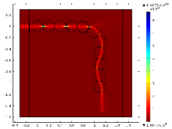
Figure 6: A right angle bend waveguide is formed by eleven Luneburg lenses. The EM wave is guided and bends at right angle through a network of lenses. The losses in this case are approximately 27% of the initial amplitude, i.e $E_{OUT}/E_{IN}=0.73$.

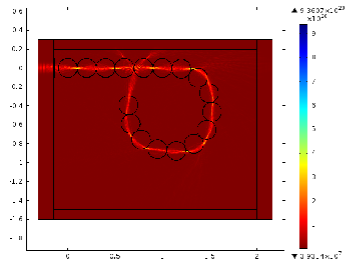
Figure 7: A full circle bend waveguide is formed by seventeen Luneburg lenses. The EM wave is guided through a circular orbit. The losses in this arrangement are approximately 30% since $E_{OUT}/E_{IN}=0.70$.

4.2 Propagation losses

In order to find how efficient is the guiding by LL waveguides we may calculate losses due to propagation through LL networks. Subsequently, we calculate numerically the absolute value of the electric field in the first and in the last lens in each arrangement. Specifically, we calculate the integrated field intensity at a cross section that is perpendicular to the propagate direction and is located in the center of each lens and compare outgoing to incoming waves. We find that in the linear case of Fig. 4,5 that $E_{OUT}/E_{IN}=0.98$. As a result, linear guiding is almost perfect. For the right angle bend waveguide of the Fig. 6 we find that $E_{OUT}/E_{IN}=0.73$ while in the circular arrangement of the Fig. 3 $E_{OUT}/E_{IN}=0.70$. We conclude that guiding is quite efficient for such sharp bends. We note that losses can be reduced further through using LLs with different radii as well as more efficient geometries that have less sharp curvatures.

4.3 Nonlinear Kerr effect in LL waveguides

As already mentioned, if the propagating wave is a Gaussian beam the focus point shifts outside of a single LL lens. To restore focusing one may use a nonlinear medium  [12, 20]. We use this approach in the LL waveguides as well. In the Fig. 8 we propagate a Gaussian beam through a linear Luneburg waveguide which is formed by three lenses in the absence of nonlinearity; we observe that the focus is shifts to the exterior of the last lens.

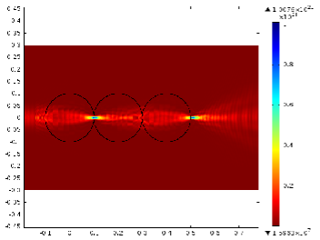
Figure 8: Linear waveguide arrangement is formed by three lenses. Simulate the propagation of the EM wave without any nonlinearity (Kerr effect). We can see that the focus points are shifted out of the surface of lenses.

In the presence of the Kerr effect the refractive index is a function of the electric field $E$, viz.

$$n(E)=n_{L}+\chi|E|^{2}$$ (16)

where $\chi$ is the nonlinear factor with units $m^{2}/V^{2}$ and $n_{L}$ is the linear part of the refractive index [12, 17, 18, 20].

For the numerical simulations we use a nonlinearity factor that makes the nonlinear part of the index of refraction, viz. the term $\chi|E|^{2}$, to be of the order of 1% of the linear part $n_{L}$. In Fig. 8 we show the shift in focusing of a LL network without nonlinear term, while in Fig. 9 the same arrangement but with the addition of nonlinearity. We note that nonlinearity shifts focusing in the LL network to the surface of the lenses [12, 20].

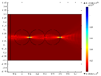
Figure 9: Linear waveguide arrangement is formed by three lenses. We simulate the propagation of the EM wave including the Kerr effect. We can see that the focus points are located again on the surface of lenses.

5 Conclusion

Luneburg lenses provide simple units for constructing GRIN-based metamaterials. The advantage of using LLs is that one may resort to an ”atomistic” picture where the lens is a single unit that has specific properties. Subsequently, these properties may be used in forming extended networks. The basic feature of LLs is their property to have a prescribed focal surface for parallel rays that lies on the lens surface. This property was used in the present study for the formation of waveguides made of Luneburg Lenses. We saw that these guides are quite versatile since they can channel light in an efficient way across different paths.

In this work we obtained an exact quasi-two dimensional solution for light trajectory through a single cylindrical LL that can be used to study propagation in arbitrary lens arrangements. This solution is parametrized on the initial entry point of light on the surface of a LL as well as the initial ray angle and gives the output location and the exit angle. One may thus form a type of input-output mapping that enables the study of propagation in various LL configurations. While this solution is analytical, it fails for backward propagation; in the latter case on may resort multiple branches, or to a parametric two dimensional solution that is found through a Hamiltonian approach. Backward propagation is now easily handled, showing that light can follow very efficiently a full circle bend waveguide constituted of LLs. Both types of solutions, viz. quasi-2D as well as true 2D give the same results in all cases compared. The ray tracing results were compared with in house FDTD as well as commercial code (COMSOL) and found good agreement. For gaussian beams the LL focusing point shifts, an artifact that can be corrected through nonlinearity also in the LL networks. The LL networks may find usueful applications in stronly focusing systems  [25].

Appendix

For completion we provide in this Appendix two alternative ways to derive the LL ray tracing solution that are based a parametric and a Helmholtz equation approach respectively.

Appendix A Parametric 2D ray solution

We use the infinitesimal arc length $ds=\sqrt{dx^{2}+dy^{2}}$ in Cartesian coordinates and further introduce the parameter $t$ as generalized time; we have $ds=\sqrt{x^{\prime 2}+y^{\prime 2}}dt$ with $\alpha^{\prime}\equiv d\alpha/dt$ and $x\equiv x(t)$, $y\equiv y(t)$ [2, 3, 11, 12, 16, 17, 19, 22]. The Fermat integral becomes

$$\mathcal{S}=\int_{A}^{B}n(x,y)\sqrt{x^{\prime 2}+y^{\prime 2}}dt$$ (17)

where $n(x,y)$ the refractive index in cartesian coordinates; the optical Lagrangian is

$$\mathcal{L}(x,y,x^{\prime},y^{\prime},t)=n(x,y)\sqrt{x^{\prime 2}+y^{\prime 2}}$$ (18)

We introduce the momenta $k_{x},k_{y}$ that are conjugate to $x,y$:

$$k_{x}=\frac{\partial\mathcal{L}}{\partial x^{\prime}}=\frac{nx^{\prime}}{\sqrt{x^{\prime 2}+y^{\prime 2}}}$$ (19)

$$k_{y}=\frac{\partial\mathcal{L}}{\partial y^{\prime}}=\frac{ny^{\prime}}{\sqrt{x^{\prime 2}+y^{\prime 2}}}$$ (20)

The Eqns. (19), (20) consist of an algebraic nonlinear system with solution:

$$k_{x}^{2}+k_{y}^{2}-n(x,y)^{2}=0$$ (21)

We rewrite Eq.(21) in vector using $\vec{r}\equiv(x,y)$ and $\vec{k}\equiv(k_{x},k_{y})$. Subsequently

$$\vec{k}^{2}-n(\vec{r})^{2}=0$$ (22)

We introduce a new function $K(\vec{r},\vec{k})$ by

$$K(\vec{r},\vec{k})=\frac{1}{2}(\vec{k}-n(\vec{r})^{2})=0$$ (23)

that has zero total differential, viz.

$$dK(\vec{r},\vec{k})=\frac{\partial K}{\partial\vec{r}}\cdot d\vec{r}+\frac{\partial K}{\partial\vec{k}}\cdot d\vec{k}=0$$ (24)

We may obtain a Hamiltonian ray tracing system by solving the Hamilton’s equations for Eq.(23) [23, 24]

$$\frac{d\vec{r}}{dt}=\frac{\partial K}{\partial\vec{k}}=\vec{k}~{}~{}~{}~{}~{}~{}~{}~{}~{}~{}~{}~{}~{}~{}~{}$$ (25)

$$\frac{d\vec{k}}{dt}=-\frac{\partial K}{\partial\vec{r}}=-\frac{1}{2}\nabla n(\vec{r})^{2}$$ (26)

where $\nabla\equiv(\frac{\partial}{\partial x},\frac{\partial}{\partial y})$ and $t$ is an effective time which is related to the real travel time as $dt=cd\tau$. Combining finally Eqns.(25)(26) we obtain

$$\ddot{\vec{r}}=\frac{c^{2}}{2}\nabla n(\vec{r})^{2}$$ (27)

where in Eq.(27) we take the derivatives respect to travel time $\tau$ thus $\dot{q}=dq/d\tau$ for arbitrary $q(\tau)$ [2, 3, 16, 17, 18, 19]. Equation (27) is a general equation for arbitrary refractive index functions $n(\vec{r})$. The explicit solution for LL will be given in the next section.

Appendix B Helmholtz wave equation approach

The stationary states of an monochromatic EM wave are given by the solutions of the following Helmholtz equation:

$$\left[\nabla^{2}+(nk_{0})^{2}\right]u(x,y)=0$$ (28)

where $u(x,y)$ is a scalar field, $n$ is the refractive index that generally depends on position, $k_{0}\equiv\omega/c=2\pi/\lambda$, where $\omega$ and $\lambda$ are the angular frequency and wavelength of the EM wave and $c$ is the velocity of light [2, 3, 17, 18, 23].

Using the well known transformation

$$u(x,y)=A(x,y)e^{i\phi(x,y)}$$ (29)

where $A,\phi$ are real, into the Helmholtz equation (28) we obtain

$$({\nabla}\phi)^{2}-(nk_{0})^{2}=\frac{\nabla^{2}A}{A}$$ (30)

$$\nabla\cdot(A^{2}{\nabla}\phi)=0~{}~{}~{}~{}~{}~{}$$ (31)

The last equation of the above system, Eq.(31), express the constancy of the flux of the vector $A^{2}\nabla\phi$ along any tube formed by the field lines of the wave vector defined through $\vec{k}={\nabla}\phi$; the latter definition turns Eq.(30) into

$$k^{2}-(nk_{0})^{2}=\frac{\nabla^{2}A}{A}$$ (32)

Using $\vec{r}\equiv(x,y)$ with the operator $\nabla=\frac{\partial}{\partial\vec{r}}\equiv(\frac{\partial}{\partial x},\frac{\partial}{\partial y})$ and introducing the function $D(\vec{r},\vec{k})$ [23].

$$D(\vec{r},\vec{k})=\frac{c}{2k_{0}}\left[k^{2}-(nk_{0})^{2}-\frac{\nabla^{2}A}{A}\right]$$ (33)

we end with a Hamiltonian ray tracing system with the following Hamilton equations:

$$\frac{d\vec{r}}{dt}=\frac{\partial D}{\partial\vec{k}}=\frac{c\vec{k}}{k_{0}}~{}~{}~{}~{}~{}~{}~{}~{}~{}~{}~{}~{}~{}~{}~{}~{}~{}~{}~{}~{}~{}~{}~{}~{}~{}~{}~{}~{}$$ (34)

$$\frac{d\vec{k}}{dt}=-\frac{\partial D}{\partial\vec{r}}={\nabla}\left[\frac{ck_{0}}{2}n^{2}+\frac{c}{2k_{0}}\frac{\nabla^{2}A}{A}\right]$$ (35)

The second term of the Eq.(35) is the Helmholtz Wave Potential [23]

$$W(r)=-\frac{c}{2k_{0}}\frac{\nabla^{2}A}{A}$$ (36)

The potential of Eq.(36) keeps the wave behavior in the ray tracing, i.e. the diffusion of the beam [23]. In the case when the space variation length $L$ of the beam amplitude $A(\vec{r})$ satisfies the condition $k_{0}L>>1$ i.e. $\lambda_{0}<<L$, the Helmholtz potential of Eq.(36) is approximately zero, thus the Eq.(31) gives the the well known eikonal equation, which is the basic equation in geometrical optics approach [7, 13, 17, 18, 19, 23].

$$(\nabla\phi)^{2}\ =(nk_{0})^{2}$$ (37)

The most important result of this approach is that the rays are not coupled any more by the Helmholtz Wave Potential and they propagate independently from one another.

Finally the equations of motion take the form

$$\frac{d\vec{r}}{dt}=\frac{c}{k_{0}}\vec{k}~{}~{}~{}~{}~{}$$ (38)

$$\frac{d\vec{k}}{dt}=\frac{ck_{0}}{2}{\nabla}n^{2}$$ (39)

which are described by the Hamiltonian

$$H(\vec{r},\vec{k})=\frac{c}{2k_{0}}\vec{k}^{2}-\frac{ck_{0}}{2}n^{2}(\vec{r})$$ (40)

Furthermore the system of equations of motion can be written in a second order ODE [2, 3, 16, 17, 18, 19].

$$\ddot{\vec{r}}=\frac{c^{2}}{2}{\nabla}n^{2}$$ (41)

Using now the LL refractive index of Eq.(1) we obtain the following equation of motion which gives the ray paths inside a LL.

$$\ddot{\vec{r}}+\frac{c^{2}}{R^{2}}\vec{r}=0$$ (42)

The solution of Eq.(43) is simple; using boundary conditions $\vec{r(0)}=\vec{r_{0}}=(x_{0},y_{0})$ and $\dot{\vec{r_{0}}}=\vec{k_{0}}=(k_{0x},k_{0y})$ we obtain:

$$\left(\begin{array}[]{c}x(t)\\ y(t)\end{array}\right)=\left(\begin{array}[]{c}x_{0}\\ y_{0}\end{array}\right)\cos(\frac{c}{R}t)+\left(\begin{array}[]{c}k_{x0}\\ k_{y0}\end{array}\right)\frac{R}{c}\sin(\frac{c}{R}t)$$ (43)

The solutions (43) in Cartesian coordinated describe elliptical orbits, in agreement with Luneburg’s theory as well as Eq. (2.2).

References

References

- [1] A.V. Kildishev, V.M Shalaev, Transformation optics and metamaterials, Physics-Uspekhi 54 53-63 (2011)
- [2] U.Leonhardt, T.Philbin, Transformation Optics and the Geometry of Light Prog. Opt 53, 69-152 (2009)
- [3] Ulf Leonhardt, Notes on conformal invisibility devices, New Journal of Physics 8 118 (2006)
- [4] D.Schurig, J.B.Pendry , D.R.Smith, Calculation of material properties and ray tracing in transformation media, OPTICS EXPRESS 14, 21 (2006)
- [5] H.Chen, C.t.Chan, P.Sheng, transformation optics and metamaterials, Nature Materials 9 (2010)
- [6] Y.Liu, T.Zentgraf, G.Bartal, X.Zhang, Transformation Plasmon Optics, Nano Letters 10, 1991-1997 (2010)
- [7] R.K.Luneburg, Mathematical Theory of Optics, University of California press, Berkeley and Los Angeles (1964)
- [8] S.P. Morgan, General Solution of the Luneburg Problem, journal of applied physics 29 9, 1358-1368 (1958)
- [9] A.Falco, S.C. Kehr, and U. Leonhardt, Luneburg lens in silicon photonics, OPTICS EXPRESS 19 6 (2011)
- [10] J.Sochacki, Exact analytical solution of the generalized Luneburg lens problem, JOSA A 73 6 (1982)
- [11] S. Takahashi, C. Chang, S. Yang, H. J. Choi, G. Barbastathis, Fabrication of Dielectric Aperiodic Nanostructured Luneburg Lens in Optical Frequencies, in Quantum Electronics and Laser Science Conference, OSA Technical Digest (CD) (Optical Society of America, 2011), paper QTuM2
- [12] H.Gao, S.Takahashi, L.Tian, G.Barbastathis, Aperiodic subwavelength Luneburg lens with nonlinear Kerr effect compensation, OPTICS EXPRESS 19, 3 (2011)
- [13] N.A. Mortensen, O. Sigmund, O. Breinbjerg, Prospects for poor-man’s cloaking with low-contrast all-dielectric optical elements, Journal of the European Optical Society-Rapid Publication 4 09008 (2009)
- [14] T.Zentgraf, Y.Liu, M.H.Mikkelsen, J.Valentine, X.Zhang, Plasmonic Luneburg and Eaton lenses, Nature Nanotechnology 6 3, 151-155 (2011)
- [15] V.Lakshminarayanan A.K.Ghatak K.Tyagarajan, Lagrangian Optics, Kluwer Academic Publishers, Springer (2002)
- [16] O. N. Stavroudis, The Mathematics of Geometrical and Physical Optics: The k-function and its Ramifications Willey-VCH, Weinheim (2006)
- [17] R.Guenther, Modern Optics, John Wiley & Sons (1990)
- [18] M.Born, E.Wolf Principles of Optics, Pergamon Press (1975).
- [19] C.G.Parazzoli, B.E.C.Koltenbah, R.B.Greegor, T.A.Lam, M.H.Tanielian, Eikonal equation for a general anisotropic or chiral medium: application to a negative-graded index-of-refraction lens with an anisotropic material JOSA B 23, 439 (2006)
- [20] H.Gao, L.Tian, B.Zhang G.Barbastathis, Iterative nonlinear beam propagation using Hamiltonian ray tracing and Wigner distribution function, OPTICS LETTERS 35 24 (2010)
- [21] A.Taflove S.C.Hagness, Computational Electrodynamics: The Finite-Difference Time-Domain method, Artech House Norwood MA 02062 (2005)
- [22] P.Stellman K.Tian G.Barbastathis, Design of Gradient Index (GRIN) Lens Using Photonic Non-Crystals, in Conference on Lasers and Electro-Optics/Quantum Electronics and Laser Science Conference and Photonic Applications Systems Technologies, OSA Technical Digest (CD) (Optical Society of America, 2007), paper JThD121
- [23] A.Orefice, R.Giovanelli, D.Ditto, Helmholtz wave trajectories in classical and quantum physics, arXiv:1105.4973v3 (2011)
- [24] H.Goldstein, C.Poole, J.Safko, Classical Mechanics, Pearson Education (2002)
- [25] L.H.Gabrielli, M.Lipson, Integrated Luneburg lens via ultra-strong index gradient on silicon, OPTICS EXPRESS 19, 21 (2011)