Universal and non-universal features of the generalized voter class for ordering dynamics in two dimensions

Abstract

By considering three different spin models belonging to the generalized voter class for ordering dynamics in two dimensions [I. Dornic, et al. Phys. Rev. Lett. 87, 045701 (2001)], we show that they behave differently from the linear voter model when the initial configuration is an unbalanced mixture up and down spins. In particular we show that for nonlinear voter models the exit probability (probability to end with all spins up when starting with an initial fraction $x$ of them) assumes a nontrivial shape. This is the first time a nontrivial exit probability is observed in two dimensional systems. The change is traced back to the strong nonconservation of the average magnetization during the early stages of dynamics. Also the time needed to reach the final consensus state $T_{N}(x)$ has an anomalous nonuniversal dependence on $x$.

I Introduction

The voter model (VM) Clifford and Sudbury (1973); Holley and Liggett (1975) is a paradigm of coarsening phenomena Bray (1994) that stands as one of the most interesting models in non-equilibrium statistical mechanics Krapivsky et al. (2010). The nature of its interest is twofold: On the one hand, it represents one of the few nontrivial non-equilibrium statistical processes that can be exactly solved in any number of dimensions Liggett (1999); Frachebourg and Krapivsky (1996). On the other hand, it has a natural application in social dynamics Castellano et al. (2009a) as a model for the formation of opinion consensus in a society initially divided in two different standpoints. The appeal of the VM is further enhanced by its connection with neutral models in genetics, ecology and linguistics Crow and Kimura (1970); Hubbell (2001); Blythe (2009). Its definition is very simple: On a regular lattice or graph, each site is endowed with a binary variable $s_{i}=\pm 1$. At each time step, a randomly chosen site copies the state of one of its nearest neighbors, chosen in its turn at random. This parameter-free dynamics can be succinctly encoded in the flipping probability $f(x_{i})$, measuring the probability that spin $i$ will flip if surrounded by a fraction $x_{i}$ of spins in the opposite state, which takes the simple linear form $f(x_{i})=x_{i}$. For this reason we will refer to it in the following as the linear voter model. Voter dynamics is thus characterized by the presence of two absorbing states (all spins either $+1$ or $-1$, the consensus states) with a $Z_{2}$ spin reversal symmetry. Moreover, since the rate of creation of $+1$ and $-1$ spins is equal, the magnetization is conserved in average.

The way in which consensus is reached in the VM can be characterized from different perspectives. From the point of view of non-equilibrium statistical mechanics, the coarsening process in the VM is marked by the absence of surface tension Dornic et al. (2001) causing an anomalous logarithmic decay of the density of interfaces in $d=2$, namely $\rho(t)\sim 1/\ln(t)$, in opposition to curvature-driven dynamics Bray (1994), which leads to an algebraic decay $\rho(t)\sim t^{-1/2}$. In the social dynamics context, on the other hand, interest is focused on the exit probability $E(x)$ Castellano et al. (2009a) (defined as the probability that the final state corresponds to all sites in state $+1$) and the consensus time $T_{N}(x)$ (the average time needed to reach consensus in a system of size $N$) when starting from fully random initial conditions with a fraction $x$ of sites in state $+1$. Conservation of magnetization implies a characteristic linear exit probability, $E(x)=x$, in any dimension $d$ Krapivsky et al. (2010), while the consensus time takes the form, for $d>1$, Blythe (2010)

$$T_{N}(x)=-N_{\mathrm{eff}}[x\ln(x)+(1-x)\ln(1-x)],$$ (1)

where $N_{\mathrm{eff}}$ is an effective factor depending on the number of sites $N$ and dimensionality $d$ Krapivsky et al. (2010).

A detailed analysis revealed that VM actually lies at the transition point between a ferromagnetic (ordered) and a paramagnetic (disordered) phase, such that infinitesimally small perturbations are able to drastically change its behavior de Oliveira et al. (1993); Drouffe and Godrèche (1999); Molofsky et al. (1999). The parameter-free nature of the VM thus led naturally to the question as whether it represents a peculiar and isolated point, or rather belongs to a more general (universal) class of models, sharing the same properties. This issue has been answered by Dornic and coworkers Dornic et al. (2001); Al Hammal et al. (2005) (see also Vázquez and López (2008); Canet et al. (2005)), who have pointed out the existence of a genuine generalized voter (GV) universality class, encompassing systems at an order-disorder transition driven only by interfacial noise, between two “dynamically equivalent” absorbing states. The dynamical equivalence between states can be enforced either by $Z_{2}$-symmetric local rules, or by global conservation of the magnetization. The linear voter model possesses both properties, but each of them separately is sufficient to ensure GV behavior. The GV class is characterized in $d=2$ by the logarithmic decay of the density of interfaces as well as by other critical exponents Dornic et al. (2001). In this generalized perspective, the GV transition for $Z_{2}$-symmetric models can be theoretically rationalized as the superposition of two independent transitions Droz et al. (2003); Al Hammal et al. (2005), an Ising transition and a directed percolation Marro and Dickman (1999) transition, whose respective symmetries are broken in unison at the GV manifold. These $Z_{2}$-symmetric models are also called nonlinear voter models, because at the transition the flipping probability $f(x_{i})$ assumes a nonlinear form.

By means of extensive numerical simulations performed for three representative models, in this paper we show that, while the GV class is well-defined in two dimensions in terms of the decay of the density of interfaces and the value of a set of the critical exponents, it also exhibits non-universal properties which depend on the microscopic details of the respective models’ definitions. The non-universality of the GV class is explicitly observed in the exit probability and the consensus time, which deviate from the linear and entropic form [Eq. (1)], respectively, observed in the linear voter model. In this respect, it is worth noticing that nontrivial shapes of the exit probability had previously been found for models in $d=1$ or at the mean-field level. Here we show for the first time that $E(x)$ can also be nontrivial in two-dimensional systems.

We have considered in particular three models representing the whole spectrum of GV class, namely the nonlinear voter model (NLV) originally devised to explore the GV manifold Dornic et al. (2001); the recently proposed non-linear $q$-voter model (qV) Castellano et al. (2009b); and the Kaya, Kabakçioǧlu, and Erzan (KKE) model Kaya et al. (2000). The first two models are $Z_{2}$-symmetric, while in the third the dynamical equivalence between absorbing states is enforced by global conservation of magnetization. Numerical simulations in the vicinity of the critical point confirm the existence of the GV universality class. In particular, measuring the exponents related to the fluctuations of the magnetization and the correlation length when approaching the critical point from the disordered and ordered phases, respectively, suggest non mean-field exponents, at odds with the claim made in Ref. Dornic et al. (2001). However, when probing the behavior of the models for unbalanced initial conditions ($x\neq 1/2$) by means of the dependence of the exit probability and of the consensus time on $x$, we observe that the originally defined GV class exhibits strong non-universal features, represented by an exit probability and the consensus time that can depend on further microscopic details of the models undergoing the GV transition. In particular, we observe that models in which conservation of average magnetization is strictly enforced, such as the KKE model, have indeed a linear $E(x)$ as the VM, but they exhibit a consensus time $T_{N}(x)$ different from the entropic form Eq. (1). On the other hand, models which exhibit $Z_{2}$-symmetry, such as the NLV and the qV models, display $E(x)$ and $T_{N}(x)$ both departing from the linear VM behavior. The non-linearity of the exit probability can be rationalized by inspecting the behavior of the average magnetization over time. Here we can see that magnetization is not conserved over short time scales, but it increases initially in the NLV model, while it decreases in the qV model. This transient behavior can be traced back to the presence of strong non-zero drift in the initial dynamical evolution starting from $x\neq 1/2$. After this initial drift has vanished, the average magnetization remains constant and the ensuing evolution is well described by a linear voter dynamics.

The paper is organized as follows: In Section II we present the results of numerical simulations for the class of non-linear voter models, determining the values of the critical exponents and showing the nontrivial $x$ dependence of the exit probability and of the consensus time. In Section III we do the same for the $q$-voter model, while Section IV is devoted to the KKE model. The final Section summarizes the results and discusses their relevance.

II The Non-linear Voter model

The characteristics of the GV class were exposed in Ref. Dornic et al. (2001) by numerical examination of a $Z_{2}$-symmetric non-linear voter model (NLV) defined it terms of a kinetic Ising model as follows: We consider a binary spin system in $d=2$, in which the probability $r_{s,h}$ that a spin $s$ flips depends on its value and the value of the local field $h$ it feels. The $Z_{2}$ symmetry imposes $r_{-s,h}=r_{s,-h}$; therefore all flipping probabilities can be encoded in the flipping probability for a $s=+1$ spin, $r_{h}\equiv r_{+1,h}$. The absence of bulk noise imposes $r_{4}=0$. The standard linear VM is given by $r_{h}=1/2-h/8$. In the general case, the NLV model depends on four free parameters, $r_{-4}$, $r_{-2}$, $r_{0}$ and $r_{2}$. In the following, we adopt the arbitrary parametrization of Ref. Dornic et al. (2001), imposing $r_{-2}=0.275$, $r_{0}=1/2$, $r_{2}=r_{-4}/4$, and taking $r_{-4}\equiv\varepsilon$ as a free tuning parameter. With this parametrization, the GV point corresponds to a critical value $\varepsilon_{c}$ separating a paramagnetic phase for $\varepsilon>\varepsilon_{c}$ from a ferromagnetic phase at $\varepsilon<\varepsilon_{c}$.

II.1 Critical point and critical exponents

As a first step in our analysis of the NLV model, we first check the results of Ref. Dornic et al. (2001) by numerically evaluating its critical GV point, and estimating the value of the corresponding critical exponents. The critical point can be estimated by monitoring the density of interfaces $\rho(t)$ and identifying $\varepsilon_{c}$ as the value leading to a logarithmic decay $\rho(t)\sim 1/\ln(t)$, separating a constant behavior ($\varepsilon>\varepsilon_{c}$) from an algebraic decay ($\varepsilon<\varepsilon_{c}$) Dornic et al. (2001). Here we propose a different approach to determine with high precision the critical point $\varepsilon_{c}$, based on the behavior of the exit probability $E(x)$. Indeed, $\varepsilon>\varepsilon_{c}$ corresponds to a disordered paramagnetic phase with, for asymptotically large systems, $E(x)=1/2$, while $\varepsilon<\varepsilon_{c}$ corresponds to an ordered ferromagnetic phase, where $E(x)=\Theta(x)$, the Heaviside theta function. Therefore, focusing on an initial density $x<1/2$, we should observe $E(x)\to 1/2$ for $\varepsilon>\varepsilon_{c}$, $E(x)\to 0$ for $\varepsilon<\varepsilon_{c}$, and $E(x)\to\mathrm{const}<1/2$ for $\varepsilon=\varepsilon_{c}$ when increasing the system size $L$.

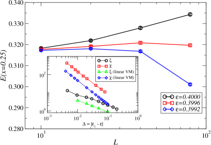
Figure 1: (Color online) Main: Finite-size scaling of the exit probability at $x=0.25$ as a function of system size in the NLV model in $d=2$, computed over at least $5\times 10^{5}$ independent realizations of the dynamics for each system size. Inset: Susceptibility and correlation length as a function of $\Delta=|\varepsilon_{c}-\varepsilon|$ on lattices of size $L=100$ and $L=5000$, respectively.

In Fig. 1 (main plot) we report the exit probability for $x=0.25$ and different values of $\varepsilon$ as a function of the lattice size $L$. A plateau is obtained for $\varepsilon\simeq 0.3996$, while larger (smaller) values of $\varepsilon$ lead to an increase (decrease) of $E(x=0.25)$ with $L$. We conclude that the critical point of the GV transition in $d=2$ for the NLV model is located at $\varepsilon_{c}=0.3996(4)$, in good agreement with the result inferred from Fig. 3(a) in Ref. Dornic et al. (2001), where a behavior for the density of interfaces with the logarithmic VM form was found.

The properties of the GV universality class can be further explored by considering several critical exponents, measured in the vicinity of the critical point $\varepsilon_{c}$. These exponents are usually defined in terms of the susceptibility, measured as the fluctuations of the magnetization $\phi=\sum_{i}s_{i}/N$, i.e.

$$\chi=L^{2}\left[\langle{\phi^{2}}\rangle-\langle{|\phi|}\rangle^{2}\right],$$ (2)

when approaching the transition from the paramagnetic, disordered phase, and the correlation length $\xi$ which, when approaching the GV manifold from the ferromagnetic, ordered phase, can be measured from the relation Dornic et al. (2001)

$$\rho(t)\sim\xi t^{-1/2}.$$ (3)

Close to the critical point, these two quantities depend on $\Delta=|\varepsilon_{c}-\varepsilon|$, defining the critical exponents

$$\chi(\Delta)\sim\Delta^{-\gamma},\qquad\xi(\Delta)\sim\Delta^{-\nu}.$$ (4)

In Fig. 1 (inset) we present the results of numerical simulations of the quantities $\xi$ and $\chi$ as a function of $\Delta$. While the determination of $\gamma$ is straightforward, the measurement of $\nu$ is hindered by extremely long pre-asymptotic effects in the curvature-driven regime, leading to a decay of $\rho(t)$ with an effective numerical exponent smaller than $1/2$ Corberi et al. (2008). Here, in order to obtain information about $\xi$, we proceed by performing a linear regression of $1/\rho^{2}(t)$ as a function of $t$, and assigning to $\xi$ the value of the slope thus obtained. Data obtained in this way (Fig. 1 (inset)) provide the exponent values $\nu\simeq 0.60$, $\gamma\simeq 1.26$. The value of $\gamma$ is in excellent agreement with early numerical values de Oliveira et al. (1993); Dornic et al. (2001), while $\nu$ is rather different from the estimate of Dornic et al. Dornic et al. (2001) and compatible with the result from de Oliveira et al. (1993). Both exponents are also quite compatible with the scaling relation $\gamma=2\nu$. With respect to the mean-field values ($\nu=1/2$, $\gamma=1$, with logarithmic corrections) proposed in Ref. Dornic et al. (2001), from our data it is difficult to make a definite discrimination for the exponent $\nu$, since the plot of $\xi$ as a function of $\Delta$ can be equally well fitted to a pure power-law with non mean-field exponent or to a mean-field value with logarithmic corrections. On the other hand, the exponent $\gamma$ seems apparently better fitted with a non mean-field power-law exponent.

To check these results we consider the linear VM in the GV manifold, which in the NLV model introduced in Dornic et al. (2001) can be approached by setting $r_{-4}=1$, $r_{0}=1/2$ and taking $r_{-2}\equiv\varepsilon\to\varepsilon_{c}=3/4$. Here the state is paramagnetic for $\varepsilon<\varepsilon_{c}$, while it is ferromagnetic for $\varepsilon>\varepsilon_{c}$. In this case, see Fig. 1 (inset), we obtain $\gamma_{\mathrm{VM}}\simeq 1.29$ and $\nu_{\mathrm{VM}}\simeq 0.62$, which confirm the universality of the GV class.

II.2 Exit probability and consensus time

The analysis presented above confirms the results of previous studies. However, it also points out a new and surprising feature, which is only evident in simulations performed out of the initial symmetric state ($x=1/2$). As we can see from Fig. 1 (main plot), the exit probability of the NLV model at criticality (on the GV manifold) computed at the non-symmetric homogeneous initial state $x=0.25$, takes a value $E(x=0.25)=0.32\pm 0.02$, i.e. larger than $0.25$, well beyond error bars. This observation hints towards a non-linear form of the exit probability, which is confirmed in Fig. 2a).

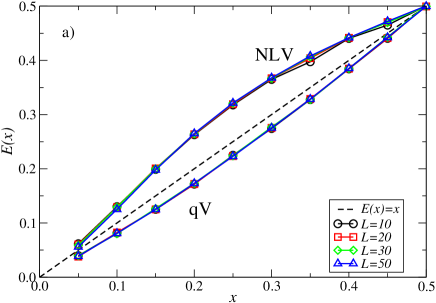
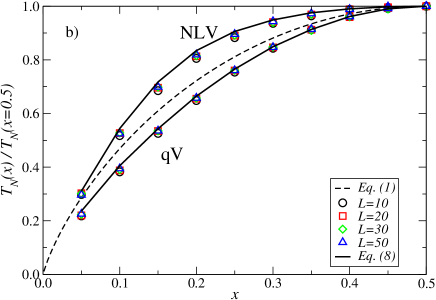
Figure 2: (Color online) (a) Exit probability as a function of the initial density for different system sizes in the NLV model and the $q=4$ qV model at the respective GV critical points. (b) Normalized consensus time as a function of $x$ for the same models.

In this plot we can see that the exit probability $E(x)$ deviates from linearity for the whole range of values of $x$. This deviation from linear VM behavior extends also to the consensus time as a function of $x$, as we can also see in Fig. 2b).

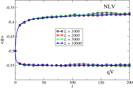
Figure 3: (Color online) Average magnetization $\phi(t)$ as a function of time for different system sizes in the NLV model and the $q=4$ qV model at the respective GV critical points, for initial conditions with magnetization $\phi(0)=-0.5$, corresponding to $x=0.25$.

This departure of the NLV model from linear VM behavior can be understood by looking in detail at the time evolution of the magnetization $\phi(t)$ in the system, starting from $x(0)=0.25$, corresponding to $\phi(0)=2x(0)-1=-0.5$, see Fig. 3. Data shows that magnetization is strongly not conserved at short times, but in fact it experiences a sharp increase until it stabilizes, for times $t\geq 100$, at a plateau with approximate value $\phi_{\infty}\approx-0.37$. The peculiar time evolution of the average magnetization (already noticed in Ref. Dornic et al. (2001)) can be related to the drift $v(\phi)$ in a Langevin representation Al Hammal et al. (2005), in the form $\partial_{t}\langle{\phi}\rangle=\langle{v(\phi)}\rangle$ Gardiner (2010). We estimate the average drift $\langle{v(\phi)}\rangle$ by computing $-2/N\sum_{i}s_{i}f(x_{i})$ (where $x_{i}$ is the fraction of neighbors of $i$ in opposite state) and we average all values of drift with the same magnetization value $\phi=1/N\sum_{i}s_{i}$. In Fig. 4 we plot $\langle{v(\phi)}\rangle$ vs $\phi$ for different system sizes in two distinct temporal regimes. For short times ($t<100$) a sharp rise is present in the vicinity of the initial magnetization. This is responsible for the initial increase of magnetization until it reaches the steady state and its conserved (in average) value. For larger values of time $t>100$ this rise is absent, and the drift takes a flat, almost vanishing form, thus ensuring conservation of magnetization.

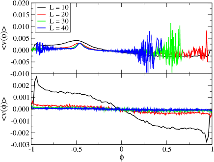
Figure 4: (Color online) Average drift as a function of the magnetization for different system sizes in the NLV model in $d=2$ at the critical point, for system starting at an initial magnetization $\phi(0)=-0.5$ ($x=0.25$). Top: $t<100$. Bottom: $t>100$.

Given the flipping probability $f(x)$, the origin of the rise for short times can be understood by considering the initial uncorrelated condition. In that case the average drift is given by

$$\langle v(\phi)\rangle_{t=0}=-\frac{2}{N}\sum_{s}\sum_{h}~{}~{}s~{}~{}f\left(\frac{4-sh}{8}\right)~{}~{}{\rm Prob}(s,h),$$ (5)

where $h$ is the local field (assuming even values between $-4$ and $4$), ${\rm Prob}(-1,h)=(1-x)\binom{4}{k}x^{k}(1-x)^{4-k}$, ${\rm Prob}(+1,h)=x\binom{4}{k}x^{k}(1-x)^{4-k}$, and $k=(4+h)/2$. In the case of the NLV model defined in Ref. Dornic et al. (2001), the flipping probability of a $+1$ spin takes the form $f_{+}(1)=r_{-4}$, $f_{+}(3/4)=r_{-2}$, $f_{+}(1/2)=r_{0}$, $f_{+}(1/4)=r_{2}$, and $f_{+}(0)=0$. Performing the summations in Eq. (5) we obtain the drift as a function of magnetization

$$N\langle v(\phi)\rangle_{t=0}=\frac{1}{8}\phi(1-\phi^{2})F(\phi),$$ (6)

where

$$F(\phi)=2(1-\phi^{2})(2r_{-2}-3r_{0})+(3+\phi^{2})(r_{-4}-4r_{2}).$$ (7)

Depending on whether $F(\phi)$ is positive or negative, the drift will have the same sign of $\phi$ or the opposite. For the NLV model, we have $r_{2}=r_{-4}/4$; therefore, in this case $F(\phi)=2(1-\phi^{2})(2r_{-2}-3r_{0})$ and it is negative for $r_{-2}<3r_{0}/2$. For the values chosen for the NLV model, this inequality is indeed satisfied, and therefore the initial drift is positive for $\phi<0$ ($x<1/2$), negative for $\phi>0$ ($x>1/2$) and vanishes for $\phi=0$ ($x=1/2$).

These results clarify the origin of the nonlinear exit probability $E(x)$ in $Z_{2}$-symmetric models. Initial conditions $x\neq 1/2$ imply a strong nonzero drift, which rapidly brings the fraction of initial spins from its initial value $x$ to a different value $x^{\prime}$. After this short transient the build up of spatial correlations cancels the drift, magnetization is conserved and the dynamics becomes identical to that of linear VM. As a consequence $E_{NLV}(x)=E_{VM}(x^{\prime})=x^{\prime}$ as witnessed by Fig. 3, where the density of $+1$ spins, starting from initial conditions $x=0.25$, reaches a plateau $x^{\prime}=(1+\phi_{\infty})/2\simeq 0.315$, in good agreement with the estimate of the exit probability, i.e. $E(0.25)\simeq 0.32$. A similar mechanism is at the origin of nonlinear exit probabilities for opinion dynamics models in $d=1$ Castellano and Pastor-Satorras (2011). The same argument allows also to estimate the deviation of the consensus time from the entropic form Eq. (1). In the short initial transient the fraction of $+1$ spins quickly converges to $x^{\prime}=E(x)$. The consensus time is essentially set by the subsequent slow ordering, which occurs as in the linear VM, hence we can write Sood and Redner (2005); Masuda et al. (2010); Blythe (2010)

$$T_{NLV}(x)=T_{VM}[E(x)].$$ (8)

Figure 2b) confirms the correctness of this theoretical estimate, and hints towards the relevance of the microscopic details of the model, which induce a strong drift at short time scales and lead in this way to nonuniversal features such as a nonlinear exit probability and anomalous consensus time.

III The $q$-voter model

In order to confirm the departure of the exit probability and of the consensus time from linear voter behavior for $Z_{2}$-symmetric models in the GV class, we consider the recently introduced non-linear $q$-voter (qV) spin model, which is defined as follows Castellano et al. (2009b): At each time step $t$, a random site $i$ is chosen; additionally $q$ nearest neighbor sites of $i$ are also randomly selected (allowing for repetition to simplify the analysis), and their spins examined. If all the $q$ neighbors are in the same state, the spin at site $i$ takes their common value. Otherwise, the spin at $i$ flips its state with probability $\varepsilon$. In any case, time is updated $t\to t+1/N$. With this definition the flipping probability in the qV model takes the form $f(x_{i},q,\varepsilon)=x_{i}^{q}+\varepsilon\left[1-x_{i}^{q}-\left(1-x_{i}\right)^{q}\right]$, where we remind that $x_{i}$ is the fraction of neighbors of site $i$ in the opposite state. Following simple mean-field arguments Castellano et al. (2009b); Al Hammal et al. (2005); Vázquez and López (2008), one can show the existence of a critical point $\varepsilon=\varepsilon_{c}(q)$, corresponding to GV behavior, separating a paramagnetic (disordered) phase for $\varepsilon>\varepsilon_{c}$ from a ferromagnetic (ordered) phase at $\varepsilon<\varepsilon_{c}$. In a $d=1$ lattice, the qV model can be exactly mapped to the model of nonconservative voters proposed in Ref. Lambiotte and Redner (2008). From here, one observe voter behavior at $\varepsilon_{c}=1/2$ for any value of $q$, while values of $\varepsilon\neq 1/2$ lead to ordering dynamics with a non-trivial, non-linear exit probability. In the more interesting case $d=2$, numerical evidence presented in Ref. Castellano et al. (2009b) for the case $q=4$ indicated the presence of a critical point at $\varepsilon_{c}\simeq 1/4$. For this value of $\varepsilon$, evidence of voter behavior was found in terms of the decay of the density of interfaces and the scaling of the correlation function, both of which are fully compatible with the VM results.

III.1 Critical point and critical exponents

Following the lines of the analysis carried out for the NLV model in Sec. II.1, we first determine precisely the critical point of $q=4$ qV model by performing a finite size scaling analysis of the exit probability at $x=0.25$.

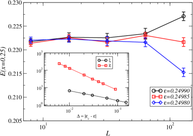
Figure 5: (Color online) Main: Finite-size scaling of the exit probability at $x=0.25$ as a function of system size in the $q=4$ qV model in $d=2$, computed over at least $5\times 10^{5}$ independent realizations of the dynamics for each system size. Inset: Susceptibility and correlation length as a function of $\Delta=|\varepsilon_{c}-\varepsilon|$ for the $q=4$ qV model on lattices of size $L=100$ and $L=5000$, respectively.

In Fig. 5 (main plot) we report the exit probability for this value of $x$ and different values of $\varepsilon$ as a function of the lattice size $L$. A plateau is obtained for $\varepsilon\simeq 0.24985$, while larger (smaller) values of $\varepsilon$ lead to an increase (decrease) of $E(x=0.25)$ with $L$. We conclude that the critical point of the GV transition in $d=2$ for the $q=4$ qV model is located at $\varepsilon_{c}=0.24985(5)$, in good agreement with the previous estimate in Ref. Castellano et al. (2009b). We further confirm the fact that the critical $q=4$ qV model belongs to the GV class by computing the exponents $\nu$ and $\gamma$, Fig. 5 (inset). We obtain the values $\nu\simeq 0.57$ and $\gamma\simeq 1.28$, in reasonable agreement with our estimates for the NLV model.

III.2 Exit probability and consensus time

As in the case of the NLV model, the exit probability at $x=0.25$ indicates the presence of a nonlinear form, taking a value $E(x=0.25)=0.222\pm 0.007$, smaller than $0.25$ beyond the estimated error bars. The non-linearity of $E(x)$ is further confirmed in Fig. 2a), where we compare the function $E(x)$ for $x<0.5$ with the linear form valid for linear VM. $E(x)$ is non-linear in the whole range of $x$ values, being independent of $L$ at this critical point $\varepsilon_{c}$. The deviation of the qV model from linear VM behavior extends, similarly to the NLV model, to the functional dependence with $x$ of the consensus time $T_{N}(x)$ at the critical point $\varepsilon_{c}$, as shown in Fig. 2b).

Noticeably, in the case of the qV model, the exit probability is smaller than $x$, in opposition to the NLV model, where we observed values $E(x)>x$. This smaller value of the exit probability is reflected in the evolution of the magnetization $\phi(t)$, see Fig. 3, which is again strongly not conserved at short times, exhibiting a sharp drop until it stabilizes, for times $t\geq 50$, at a plateau with approximate value $\phi_{\infty}\approx-0.55$.

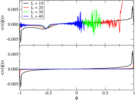
Figure 6: (Color online) Average drift as a function of the magnetization for different system sizes in the $q=4$ voter model in $d=2$ at the critical point, for system starting at an initial magnetization $\phi(0)=-0.5$ ($x=0.25$). Top: $t<50$. Bottom: $t>50$.

The time evolution of the average magnetization is again related with the drift $v(\phi)$. In Fig. 6 we plot $\langle{v(\phi)}\rangle$ vs $\phi$ for different system sizes in two distinct temporal regimes. For short times ($t<50$) a sharp dip is present in the vicinity of the initial magnetization. This is responsible for the initial decrease of magnetization until it reaches the steady state and its conserved (in average) value. For larger values of time ($t>50$) this dip is absent, and the drift takes a flat, almost vanishing form, thus ensuring conservation of magnetization.

The dip in the drift a short times can also be understood by computing the drift in the initial uncorrelated condition. From Eqs. (6) and (7), and considering that for the qV model the flipping rates $r_{i}$ can be written as $r_{-4}=1$, $r_{-2}=3(27+58\varepsilon)/256$, $r_{0}=(1+14\varepsilon)/16$, $r_{2}=(1+174\varepsilon)/256$, and $r_{4}=1$, we obtain

$$F(\phi)=\frac{3}{32}\left[(1-2\varepsilon)\phi^{2}+41-114\varepsilon\right],$$ (9)

which is a positive function for all $\phi$ for $\varepsilon<41/114$. Thus, for $\varepsilon=\varepsilon_{c}$, we find that the initial drift is negative for $\phi<0$ ($x<1/2$), positive for $\phi>0$ ($x>1/2$) and vanishes for $\phi=0$ ($x=1/2$). Again, for the qV model the nonlinear exit probability and the anomalous consensus time can be related through the argument leading to Eq. (8). Indeed, for $x=0.25$, from Fig. 3 we read a stationary large time magnetization $\phi_{\infty}\approx-0.55$, corresponding to $x^{\prime}\simeq 0.225$, is in good agreement with the estimate of the exit probability, i.e. $E(0.25)\simeq 0.222$. Eq. (8) is again valid for the whole range of values of $x$, as shown in Fig. 2.

IV Conserved magnetization: the Kaya, Kabakçioǧlu, and Erzan model

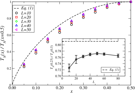
Figure 7: (Color online) Main plot: Consensus time as a function of $x$ for different system sizes in the KKE model at the delocalization transition in $d=2$. Inset: Evolution of $T_{N}(x)/T_{N}(0.5)$ for $x=0.25$ as a function of the system size $L$.

From the analysis of the results obtained for the NLV and qV models, we expect that any $Z_{2}$-symmetric model belonging to the GV class and endowed with a nonlinear flipping probability $f(x_{i})$ will exhibit a strictly nonlinear exit probability and a “non-entropic” form of the consensus time $T_{N}(x)$. By the same token, it is clear that in other type of models belonging to the GV class, conservation of the average magnetization will guarantee a linear exit probability Krapivsky et al. (2010), as for linear VM. The question naturally arises about the form of the consensus times in those models in the GV class in which conservation of magnetization is enforced.

To answer this question we have considered the KKE interface model at the delocalization transition Kaya et al. (2000), which can be formulated in terms of a spin systems as follows: At each time step a spin $s_{i,j}$ and one of its neighbors are randomly selected; if they are equal nothing happens, otherwise the number $n^{+}$ of positive neighbors of the negative spin is computed and, with probability $1/n^{+}$, $s_{i,j}$ and the neighbor are made equal. This model belongs to the GV class, as has been shown in Ref. Dornic et al. (2001), where a logarithmic decay of the density of interfaces was observed. In Fig. 7 we plot the rescaled consensus time as a function of $x$ for different system sizes. These results indicate that again the consensus time deviates from the form expected in linear VM. The deviation from the behavior given by Eq. (1) should be attributed again to relevant microscopic details of the model. However, the mechanism inducing the deviation is here necessarily different from the one responsible for the deviation for the NLV and qV models (i.e. initial short timescale nonconservation of magnetization). Its investigation constitutes an interesting line for future research.

V Conclusions

In summary, in this paper we have shown, using large scale numerical simulations of three different spin models, that different subclasses of the generalized voter class for ordering dynamics actually exhibit different behaviors when unbalanced initial conditions are considered. All elements of the GV class are broadly characterized by lack of surface tension and a logarithmic decay of the density of interfaces in $d=2$. However, when looking at the exit probability and the consensus time, two types of behavior occur. In one subclass, encompassing systems, such as KKE, with no $Z_{2}$ symmetry but magnetization conserved on average, the consensus time differs from the entropic form characterizing the VM, while the exit probability is linear. In the other subclass, composed by systems with $Z_{2}$ symmetry and nonlinear form of the flipping probability $f(x)$, both the exit probability and the consensus time differ from the VM. This variation is essentially due to a nonconservation of magnetization during a short initial transient. The buildup of spatial correlations rapidly leads to an effective cancellation of the drift, so that the subsequent evolution is the same as for the linear VM, but starting from $x^{\prime}\neq x$ so that $E(x)$ and $T(x)$ are modified. To the best of our knowledge the results for the NLV and qV models reported here constitute the first example of a dynamics in $d=2$ with an exit probability different (in the large system size limit) from the step-function (typical of dynamics driven by surface tension) or the linear shape of VM. Nontrivial shapes were previously found only in $d=1$ Lambiotte and Redner (2008); Slanina et al. (2008) and in mean-field, but not in $d=2$. Finally, our numerical estimates of the critical exponents associated to the GV transition suggest a value of the $\gamma$ exponent possibly different from the mean-field value previously supposed to hold. Further research work is needed to fully clarify this issue, based on numerical simulations on systems sizes beyond those used in the present work, which are at the boundary of our computational limits.