Ginzburg-Landau theory of the zig-zag transition in quasi-one-dimensional classical Wigner crystals

Abstract

We present a mean-field description of the zig-zag phase transition of a quasi-one-dimensional system of strongly interacting particles, with interaction potential $r^{-n}e^{-r/\lambda}$, that are confined by a power-law potential ($y^{\alpha}$). The parameters of the resulting one-dimensional Ginzburg-Landau theory are determined analytically for different values of $\alpha$ and $n$. Close to the transition point for the zig-zag phase transition, the scaling behavior of the order parameter is determined. For $\alpha=2$ the zig-zag transition from a single to a double chain is of second order, while for $\alpha>2$ the one chain configuration is always unstable and for $\alpha<2$ the one chain ordered state becomes unstable at a certain critical density resulting in jumps of single particles out of the chain.

I Introduction

During the last two decades the interest in self-organized systems has increased enormously both experimentally and theoretically, due to its importance in solid-state physics, plasma physics as well as in atomic physics. Wigner crystals are an elementary example of self-organization which has been realized in very diverse systems as e.g. electrons on liquid helium022_ikegami , by using the well-known Paul and Penning traps020_itano ; 021_waki to confine ions in a limited region, in dusty plasma033_dubin , and more recently using static and radio-frequency electromagnetic potentials where crystallization was realized through laser cooling023_mortensen . Additionally it has been proposed that these structures can be used for a possible implementation of a scalable quantum information processor024_cirac ; 026_leibfried , and as quasi-one-dimensional (Q1D) Wigner crystals025_taylor . The theoretical analysis of these crystal structures has been realized previously, for 3D005_cornelissens ; 008_hasse , 2D002_schweigert ; 004_schweigert ; 009_partoens and Q1D003_piacente ; 014_fishman systems. From those studies it was shown that structural phase transitions can be induced by varying the strength of the external confinement potential and/or the density of particles.

In the present paper we concentrate on the ordered state of identical particles that are confined in a Q1D channel. When the particles move in 2D and are confined by a parabolic003_piacente or hard wall034_yang potential in one of the in-plane directions the particles arrange themselves in parallel chains at low temperature. Previously, it was found003_piacente that with increasing density (or decreasing strength of the confinement potential) the system passes through a sequence of first and second order phase transitions where at each point the number of chains changes. Of particular interest to us is the one chain to two chain transition which for a parabolic confinement potential was found to be a second order phase transition which occurs as a zig-zag transition. Such a transition was observed experimentally030_valkering ; 031_chan ; 028_lutz ; 029_lutz in systems with a finite number of particles, and the effects of a narrow channel and finite size of the system on the diffusion was recently analyzed in Refs. [032_lucena, ] and [027_saintjean, ]. Recently it was found theoretically006_piacente that the analytic form of the confinement potential is very important for the occurrence of the zig-zag transition and the order of the phase transition. Therefore, in the present paper we generalize the previous analysis to an arbitrary power law confinement potential (i.e. $y^{\alpha}$) and also to arbitrary inter-particle interaction which we model by $r^{-n}e^{-r/\lambda}$, which simulates most of the relevant experimental particle-particle interactions. With this model potential we can simulate both short range and long range interactions.

We are interested in the behavior of the system at the zig-zag transition i.e. at the critical point. This can be viewed as a spontaneous symmetry breaking and we will cast the problem into a mean field theory based on Landau’s theory of phase transitions. In this way we will construct a Ginzburg-Landau theory, for the single to two chains transition in a quasi-one-dimensional system of interacting particles. We generalize the approach of Refs. [014_fishman, ] and [011_delcampo, ] to arbitrary power-law confinement and inter-particle interaction potential. We obtain a Ginzburg-Landau equation for the order parameter close to the transition point, and determinate all the relevant parameters in this equation. The order parameter is the distance of the particles from the trap axis. By considering a large number of particles and using the local density approximation, we can consider the crystal as a continuum, so that the order parameter becomes a field.

The present paper is organized as follows. In Sect. II we describe the model system and using Landau theory we find the behavior of the system close to the transition point. Next we derive a Ginzburg-Landau equation for the system finding the dispersion relation. In Sect. III the results for the critical point and the normal mode spectrum are discussed. Our conclusions and a discussion of possible quantum effects are given in Sect. IV.

II Theoretical Framework

We consider a two-dimensional system consisting of $N$ particles with mass $m$ and charge $q$, which are allowed to move in the $x-y$ plane. The charged particles interact through a repulsive interaction potential; they are free to move in the $x$ direction but are confined by a one-dimensional potential which limits their motion in the $y$ direction. The total energy of the system is given by:

$$E=\frac{1}{2}m\sum_{i=1}^{N}{\mathbf{\dot{r}}_{i}^{2}}+V_{conf}+V_{int},$$ (1)

where $V_{conf}$ and $V_{int}$ are the confinement and interaction potential respectively, given by

$$V_{conf}=\frac{1}{2}m\upsilon_{t}^{2}R^{2}\sum_{i=1}^{N}{\frac{|y_{i}|^{\alpha}}{R^{\alpha}}},$$ (2a)

$$V_{int}=\sum_{i=1}^{N}\sum_{j>i}^{N}V_{pair}(r_{ij}),$$ (2b)

where $V_{pair}(r_{ij})$ represents the inter-particle interaction. The latter one will be taken as a screened power-law potential as follows:

$$V_{pair}=\frac{q^{2}}{\epsilon R}\frac{R^{n}e^{-r_{ij}/\lambda}}{r_{ij}^{n}},$$ (3)

where $r_{ij}=|\mathbf{r}_{i}-\mathbf{r}_{j}|$ represents the relative position between the $i$-th and the $j$-th particle, the exponent $n$ is an integer and $\epsilon$ is the dielectric constant of the medium the particles are moving in. In the above, $R$ is an arbitrary length parameter which we introduced to guarantee the right units. The energy can be written in dimensionless form

$$E=\sum_{i=1}^{\infty}{\mathbf{\dot{r}}_{i}^{2}}+\upsilon^{2}\sum_{i=1}^{N}{|y_{i}|^{\alpha}}+\sum_{i=1}^{N}{\sum_{j>i}^{N}{\frac{e^{-\kappa r_{ij}}}{r_{ij}^{n}}}},$$ (4)

with dimensionless frequency $\upsilon$ given by $\upsilon=\upsilon_{t}/\omega_{0}$, while $\omega_{0}$ measures the strength of the confinement potential and $t_{0}=1/\omega_{0}$ is the unit of time. The energy is expressed in units of $E_{0}=\left(m\omega_{0}^{2}/2\right)^{n/(n+\alpha)}\left(q^{2}/\epsilon\right)^{\alpha/(n+\alpha)}R^{(2n-\alpha)/(n+\alpha)}$ and all distances are expressed in units of $r_{0}=\left(2q^{2}/m\omega_{0}^{2}\epsilon\right)^{1/(n+\alpha)}R^{(n+\alpha-3)/(n+\alpha)}$. Additionally, the dimensionless parameter $\kappa=r_{0}/\lambda$ represents the screening parameter of the potential. Limiting cases of this interaction potential are: Yukawa potential ($n=1$), power-law potential ($\kappa=0$), Coulomb potential ($\kappa=0,n=1$) and dipole interaction ($\kappa=0,n=3$). We introduce a dimensionless linear density $\eta$ defined as the number of particles per unit of length along the unconfined direction.

In Ref. [006_piacente, ] it was demonstrated that for $\alpha>2$ the one-chain configuration is not stable for any values of $\eta$ and $\upsilon$. Only for $\alpha=2$ the system exhibits a continuous transition from the one-chain to the two-chain configuration (i.e. zig-zag transition) at a transition point defined by a critical density ($\eta_{c}$) or a critical frequency ($\upsilon_{c}$). For $\alpha<2$ the ground state configuration of the particles is, below $\eta_{c}$ or above $\upsilon_{c}$, arranged in a single chain. Beyond this critical point particles are expelled one by one from this chain to positions parallel to the chain.

For the special case of $\alpha=2$ and before the transition point, the particles crystallize around the minimum point of the confinement potential $V$, at the positions $\mathbf{r}_{i}^{linear}=(i/\eta)\mathbf{e_{x}}$ with $i$ an integer. The stability of the linear chain along the $x$ axis requires a relative transverse trap frequency exceeding a threshold value $\upsilon_{c}$ or a linear density smaller than $\eta_{c}$. At this critical point, the configuration has a structural instability, such that for $\upsilon<\upsilon_{c}$ or $\eta>\eta_{c}$ the particles are organized in a zig-zag structure, ordered in two chains with equilibrium positions $\mathbf{r}_{i}^{zigzag}=(i/\eta)\mathbf{e_{x}}+(-1)^{i}(c/\eta)\mathbf{e_{y}}$, where $c$ is a real and positive constant, $d=c/\eta$ represents the distance of each particle from the confinement potential minimum and $D=2d$ indicates the lateral separation between the two chains.

II.1 Landau Theory for the zig-zag transition

For the case $\alpha=2$ and near the zig-zag regime we follow the Landau theory approach of Ref. [006_piacente, ], and expand the total potential energy of the system as a function of the order parameter $c$ in a polynomial i.e. $V(c)=V_{1ch}-Ac^{2}+Bc^{4}$, where $V_{1ch}$ represents the potential energy for the one-chain configuration. Minimizing the potential energy we obtain the condition

$$2\sum_{j=0}^{\infty}{\left[n\eta^{n}+\kappa\eta^{n-1}(2j+1)\right]\frac{e^{-\kappa\frac{2j+1}{\eta}}}{\left(2j+1\right)^{n+2}}}-\frac{\upsilon^{2}}{\eta^{2}}=0.$$ (5)

From this equation we obtain the value of $\eta_{c}(\upsilon)$ or $\upsilon_{c}(\eta)$ at which the single chain configuration becomes unstable. Considering $\eta_{c}$ and expanding the potential energy around this critical value, we find that the order parameter close to the transition point is given by

$$c=Y(\upsilon:n,\kappa)|\eta-\eta_{c}|^{\frac{1}{2}},$$ (6)

with $Y(\upsilon;n,\kappa)=\sqrt{Y_{B}Y_{C}-Y_{A}Y_{D}}/Y_{B}$ where $Y_{A}=n\eta_{c}^{n}S_{2}+\eta_{c}^{n-1}\kappa S_{1}-\upsilon^{2}/2\eta_{c}^{2}$, $Y_{B}=2n(n+2)\eta_{c}^{n}S_{4}+2(2n+1)\eta_{c}^{n-1}\kappa S_{3}+2\eta_{c}^{n-2}\kappa^{2}S_{2}$, $Y_{C}=n^{2}\eta_{c}^{n-1}S_{2}+(2n-1)\eta_{c}^{n-2}\kappa S_{1}+\eta_{c}^{n-3}\kappa^{2}S_{0}+\upsilon^{2}/\eta_{c}^{3}$, $Y_{D}=2n^{2}(n+2)\eta_{c}^{n-1}S_{4}+2[n(3n+1)-1]\eta_{c}^{n-2}\kappa S_{3}+2(3n-1)\eta_{c}^{n-3}\kappa^{2}S_{2}+2\eta_{c}^{n-4}\kappa^{3}S_{1}$, with

$$S_{k}=\sum_{i=0}^{\infty}\frac{e^{-\kappa\frac{2i+1}{\eta_{c}}}}{(2i+1)^{n+k}}.$$ (7)

The value of $Y=Y(\upsilon;n,\kappa)$ is plotted in Fig. 1 as function of $\kappa$ for different values of $n$ and a fixed value $\upsilon=1$. Notice that the curves $Y(n,\kappa)$ for different values of $n$ cross each other at some value of $\kappa$. The critical exponent of the order parameter of the zig-zag transition, Eq. (6), was verified experimentally on a low dimensional dusty plasma in Ref. [035_sheridan, ] and theoretically in Refs. [006_piacente, ], [014_fishman, ], [036_closson, ] and [037_sheridan, ].

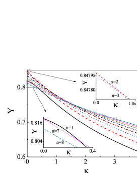
Figure 1: (Color online) The proportionality coefficient $Y(\upsilon;n,\kappa)$ as a function of $\kappa$ for different values of $n$ with $\upsilon=1$

.

II.2 Ginzburg-Landau Lagrangian for the zig-zag phase transition

Recently, this zig-zag transition (for $\alpha=2$, $\kappa=0$ and $n=1$) was cast into a mean-field description resulting in similar expressions as in the Landau theory of phase transitions. This resulted in a one-dimensional Ginzburg-Landau type non-linear field theory011_delcampo . Here, we will extend the previous calculation to the more general problem described by the energy Eq. (4). We start by considering the system in the situation that the one-chain configuration is stable but that it is close to the transition point. The equilibrium positions of all the particles are along the $x$-axis. We consider small oscillations around the equilibrium position of each particle as follows $x_{i}^{lin}=(i/\eta)+x_{i}$ and $y_{i}^{lin}=0+y_{i}$. Then the relative position between the particles can be written as follows

$$r_{ij}=\left[1+\frac{\tau_{ij}+\epsilon_{ij}}{A_{ij}}\right]^{1/2}(A_{ij})^{1/2},$$ (8)

with $A_{ij}=(\Delta_{ij})^{2}$, $\tau_{ij}=2\Delta_{ij}(x_{i}-x_{j})$ and $\epsilon_{ij}=(x_{i}-x_{j})^{2}+(y_{i}-y_{j})^{2}$, where ${\Delta_{ij}=(i-j)/\eta}$. Now, we assume that the vibration amplitudes in the axial and transverse direction are much smaller than the distance between the particles, i.e. $\tau_{ij},\>\epsilon_{ij}\ll A_{ij}$. We expand Eq. (8) and the exponential term as follows

$$r_{ij} \approx \Delta_{ij}+(x_{i}-x_{j})$$ (9)

$$+\left(1-\frac{(x_{i}-x_{j})}{\Delta_{ij}}+\frac{(x_{i}-x_{j})^{2}}{(\Delta_{ij})^{2}}\right)\frac{(y_{i}-y_{j})^{2}}{2\Delta_{ij}},$$

$$e^{-\kappa r_{ij}}\approx e^{-\kappa\Delta_{ij}} \left[1-\kappa(x_{i}-x_{j})+\kappa^{2}\frac{(x_{i}-x_{j})^{2}}{2}\right.$$ (10)

$$-\left.\kappa\frac{(y_{i}-y_{j})^{2}}{2\Delta_{ij}}\right],$$

and similar the $n$-th power of the inverse of Eq. (8) i.e. $1/r_{ij}^{n}$, as a Newton binomial around the equilibrium positions. These expansions result in a decomposition of the total potential as

$$V=\upsilon^{2}\sum_{i=1}^{\infty}{|y_{i}|^{\alpha}}+\sum_{l}^{\infty}V_{int}^{(l)},$$ (11)

where the label $l$ indicates the order of the expansion. Each order of the expansion of the interaction potential can be written as

$$V_{int}^{(l)}=\frac{1}{2}\sum_{i\neq j}^{\infty}W_{ij}^{(l)},$$ (12)

where the expansion terms up to fourth order are given by

$$W_{ij}^{(0)} = \frac{e^{-\kappa\Delta_{ij}}}{\Delta_{ij}^{n}},$$

$$W_{ij}^{(1)} = -\frac{e^{-\kappa\Delta_{ij}}}{(\Delta_{ij})^{n+1}}[\vartheta_{ij}n+\kappa\Delta_{ij}](x_{i}-x_{j}),$$

$$W_{ij}^{(2)} = \frac{e^{-\kappa\Delta_{ij}}}{2(\Delta_{ij})^{n+2}}\left[\left(n(n+1)-2\vartheta_{ij}n\kappa\Delta_{ij}+\kappa^{2}\Delta_{ij}^{2}\right)(x_{i}-x_{j})^{2}-\left(n+\kappa\Delta_{ij}\right)(y_{i}-y_{j})^{2}\right],$$

$$W_{ij}^{(3)} = \frac{e^{-\kappa\Delta_{ij}}}{2(\Delta_{ij})^{n+3}}n(x_{i}-x_{j})\bigglb[-\left(\frac{\vartheta_{ij}}{3}(n^{2}+3n+2)+(n+1)\kappa\Delta_{ij}+\vartheta_{ij}\kappa^{2}\Delta_{ij}^{2}\right)(x_{i}-x_{j})^{2}$$

$$+\left(\vartheta_{ij}(n+2)+\kappa\Delta_{ij}\right)(y_{i}-y_{j})^{2}\biggrb],$$

$$W_{ij}^{(4)} = \frac{e^{-\kappa\Delta_{ij}}}{2(\Delta_{ij})^{n+4}}n\left[\left(\frac{1}{12}(n^{3}+6n^{2}+11n+6)+3(n^{2}+3n+2)\kappa\Delta_{ij}+2(n+1)\kappa^{2}\Delta_{ij}^{2}\right)(x_{i}-x_{j})^{4}\right.$$

$$\left.-\left(\frac{1}{2}(n^{2}+5n+6)+(9(n+2)\vartheta_{ij}+2(n+1))\kappa\Delta_{ij}+2\kappa^{2}\Delta_{ij}^{2}\right)(x_{i}-x_{j})^{2}(y_{i}-y_{j})^{2}\right.$$

$$\left.+\left(\frac{1}{4}(n+2)+2\kappa\Delta_{ij}\right)(y_{i}-y_{j})^{4}\right],$$

With ${\vartheta_{ij}=\Delta_{ij}/|\Delta_{ij}|}$. It is sufficient to restrict ourselves to terms up to the fourth order and thus the potential can be written as $V_{int}\approx V_{int}^{(0)}+V_{int}^{(1)}+V_{int}^{(2)}+V_{int}^{(3)}+V_{int}^{(4)}$.

II.2.1 Representation in reciprocal space

Now we assume that the particles are pinned in the longitudinal direction and that they can only oscillate in the transverse direction ($x_{i}=0$). Therefore, their normal axial modes can be neglected and we can discard the coupling to the longitudinal modes. In this regime, we find that $W_{ij}^{(0)}=e^{-\kappa\Delta_{ij}}/(\Delta_{ij}^{n})$, $W_{ij}^{(1)}=0$, $W_{ij}^{(2)}=-\left(n+\kappa\Delta_{ij}\right)(y_{i}-y_{j})^{2}e^{-\kappa\Delta_{ij}}/(2(\Delta_{ij})^{n+2}),W_{ij}^{(3)}=0$, and $W_{ij}^{(4)}=n\left[(n+2)+8\kappa\Delta_{ij}\right](y_{i}-y_{j})^{4}e^{-\kappa\Delta_{ij}}/(8(\Delta_{ij})^{n+4})$.

In order to find the representation in reciprocal space, we define the normal modes of vibration in the transversal direction with wavevector $k$ as $\Psi_{k}=\psi^{(+)}_{k}-i\psi^{(-)}_{k}$ with amplitude $|\psi_{k}|^{2}=\psi^{(+)2}_{k}+\psi^{(-)2}_{k}$. Following the standard process to find this representation as shown in e.g. Ref. [014_fishman, ] and using Plancherel’s theoremB01_Yosida for the confinement potential transformation, the different terms of the potential become

$$V_{conf} = \frac{\upsilon^{2}}{\sqrt{N}}\sum_{k>0}|\psi_{k}|^{\alpha},$$ (13a)

$$V_{int}^{(1)} = 0,$$ (13b)

$$V_{int}^{(2)} = \sum_{k>0}\omega_{\perp}(n,\kappa,k)^{2}\psi_{k}^{2},$$ (13c)

$$V_{int}^{(3)} = 0,$$ (13d)

$$V_{int}^{(4)} = \sum_{k_{1}+k_{2}+k_{3}+k_{4}=0}{A(k_{1},k_{2},k_{3},k_{4})\prod_{m=1}^{4}\psi_{{}_{k_{m}}}},$$ (13e)

where $\omega_{\perp}(n,\kappa,k)^{2}=-\omega(n,\tilde{\kappa},k)^{2}$, $A(k_{1},k_{2},k_{3},k_{4})=n\eta^{n+4}[(n+2)A_{0}(k_{1},k_{2},k_{3},k_{4})+8\tilde{\kappa}A_{1}(k_{1},k_{2},k_{3},k_{4})]/8$, with $\tilde{\kappa}=\kappa/\eta$ and

$$\omega(n,\tilde{\kappa},k)^{2}=2\eta^{n+2} \bigglb[ n\sum_{j=1}^{\infty}\frac{e^{-j\tilde{\kappa}}}{j^{n+2}}\sin^{2}\left(j\frac{k}{2}\right)$$ (14a)

$$+ \kappa\sum_{j=1}^{\infty}\frac{e^{-j\tilde{\kappa}}}{j^{n+1}}\sin^{2}\left(j\frac{k}{2}\right)\biggrb],$$

$$A_{0}(k_{1},k_{2},k_{3},k_{4}) = \frac{2}{N}\sum_{j>0}{\frac{e^{-j\tilde{\kappa}}}{j^{n+4}}\prod_{m=1}^{4}{\sin\left(j\frac{k_{m}}{2}\right)}},$$

$$A_{1}(k_{1},k_{2},k_{3},k_{4}) = \frac{2}{N}\sum_{j>0}{\frac{e^{-j\tilde{\kappa}}}{j^{n+3}}\prod_{m=1}^{4}{\sin\left(j\frac{k_{m}}{2}\right)}},$$

Due to the condition that the motion of the particles are restricted to the longitudinal direction it becomes apparent that the first and third order term of the interaction potential will be zero, and additionally we know that the first derivative equals zero because it is the necessary condition to have an equilibrium configuration.

II.2.2 Minimum frequency of the interaction potential

From the definition of $\omega_{\perp}(n,\kappa,k)^{2}$ we find that its minimum value is located at $k_{0}=\pi$. Lets expand for $k$ around this value ($k=k_{0}-\delta k$), and we obtain

$$\omega_{\perp}(n,\kappa,k_{0}-\delta k)^{2} = \omega_{\perp}(n,\tilde{\kappa},k_{0})^{2}$$ (15a)

$$+h(n,\tilde{\kappa})^{2}\delta k^{2}+{\footnotesize O(\delta k^{4})},$$

$$A(k_{1},k_{2},k_{3},k_{4}) = \frac{1}{2N}\mathcal{A}(n,\tilde{\kappa})+O(\delta k^{2}),$$ (15b)

where $\omega_{\perp}(n,\tilde{\kappa},k_{0})^{2}=-\varpi(n,\tilde{\kappa})^{2}$ with

$$\varpi(n,\tilde{\kappa})^{2} = \left(\frac{\eta}{2}\right)^{n+2}e^{-\tilde{\kappa}}\left[2n\Phi\left(e^{-2\tilde{\kappa}},n+2,\frac{1}{2}\right)+4\tilde{\kappa}\Phi\left(e^{-2\tilde{\kappa}},n+1,\frac{1}{2}\right)\right],$$ (16a)

$$h(n,\tilde{\kappa})^{2} = \left(\frac{\eta}{2}\right)^{n}\sum_{j=1}^{2}(-1)^{j+1}e^{-j\tilde{\kappa}}\left[\frac{n}{2}\Phi\left(e^{-2\tilde{\kappa}},n,\frac{j}{2}\right)+\tilde{\kappa}\Phi\left(e^{-2\tilde{\kappa}},n-1,\frac{j}{2}\right)\right],$$ (16b)

$$\mathcal{A}(n,\tilde{\kappa}) = \left(\frac{\eta}{2}\right)^{n+4}ne^{-\tilde{\kappa}}\left[\left(\frac{n}{2}+1\right)\Phi\left(e^{-2\tilde{\kappa}},n+4,\frac{1}{2}\right)+8\tilde{\kappa}\Phi\left(e^{-2\tilde{\kappa}},n+3,\frac{1}{2}\right)\right],$$ (16c)

where $\Phi(z,s,a)$ is the Lerch transcendent defined as $\Phi\left(z,s,a\right)=\sum_{k=0}^{\infty}{z^{k}/\left(k+a\right)^{s}}$. In Table 1 we show the limiting behavior of these terms. It is important to note that the square of the transverse frequency is negative.

Table 1: Behavior of the coefficients in the Ginzburg-Landau equation in two limiting cases, where $\tilde{\kappa}=\kappa/\eta$.

	$\tilde{\kappa}\ll 1$	$\tilde{\kappa}\gg 1$
$\varpi(n,\tilde{\kappa})^{2}$	$2n\left(\frac{\eta}{2}\right)^{n+2}e^{-\tilde{\kappa}}\sum_{j=0}^{\infty}\frac{1-2j\tilde{\kappa}}{(j+1/2)^{n+2}}$	$2n\eta^{n+2}\tilde{\kappa}e^{-\tilde{\kappa}}$
$h(n,\tilde{\kappa})^{2}$	$\frac{n}{2}\left(\frac{\eta}{2}\right)^{n}\sum_{j=0}^{\infty}\left(1-2j\tilde{\kappa}\right)\left(\frac{1}{(j+1/2)^{n}}-\frac{1}{(j+1)^{n}}\right)$	$\left(\frac{\eta}{2}\right)^{n}\tilde{\kappa}e^{-\tilde{\kappa}}\sum_{j=0}^{\infty}\frac{e^{-2j\tilde{\kappa}}}{(j+1/2)^{n-1}}$
$\mathcal{A}(n,\tilde{\kappa})$	$n\left(\frac{n}{2}+1\right)\left(\frac{\eta}{2}\right)^{n+4}\sum_{j=0}^{\infty}\frac{1-2j\tilde{\kappa}}{(j+1/2)^{n+4}}$	$8n\left(\frac{\eta}{2}\right)^{n+4}\tilde{\kappa}e^{-\tilde{\kappa}}\sum_{j=0}^{\infty}\frac{e^{-2j\tilde{\kappa}}}{(j+1/2)^{n+4}}$

II.2.3 Stability of the system

The system is stable when the second order term of the total potential energy (i.e. the coefficient of $\psi_{k}^{2}$) is minimum. For the parabolic case ($\alpha=2$) the confinement potential term contributes to the second order of the total potential energy, then

$$V^{(2)}=\sum_{k>0}\omega_{\perp}(n,\kappa,k)^{2}\psi_{k}^{2},$$ (17)

where the transverse frequency is

$$\omega_{\perp}(n,\kappa,k)^{2}=\upsilon^{2}-\omega(n,\tilde{\kappa},k)^{2}$$ (18)

and we note that its minimum value is reached for $k_{0}=\pi$. Thus the critical value for the confinement frequency is given by

$$\upsilon_{c}^{2}(n,\kappa)=\varpi(n,\tilde{\kappa})^{2}.$$ (19)

When $\upsilon>\upsilon_{c}$ the ground state configuration is a one-chain organization of the particles. For $\upsilon<\upsilon_{c}$ the linear chain is unstable and the particles are arranged in a two-chain structure through a zig-zag organization. When $\upsilon$ is sufficiently close to the critical value $\upsilon_{c}$, an effective potential can be derived for the transverse normal modes $\psi_{k}$ with wavevector $\tilde{k}=k_{0}-\delta k$, such that $\delta k\ll 1$. The second order term of the effective potential is given by Eq. (17), where its coefficient, Eq. (15a), can now be written as follows

$$\omega_{\perp}(n,\kappa,k_{0}-\delta k)^{2}=\delta_{\upsilon}(n,\tilde{\kappa})+h(n,\tilde{\kappa})^{2}\delta k^{2},$$ (20)

where $\delta_{\upsilon}(n,\tilde{\kappa})=\upsilon^{2}-\upsilon_{c}(n,\tilde{\kappa})^{2}$. In the limiting case of a Coulomb inter-particle potential ($\kappa=0$, $n=1$) and considering $\eta=1$, we find $\upsilon_{c}(1,0)=\sqrt{7\zeta(3)}/2=1.45038$, $h(1,0)=\sqrt{log(2)/2}=0.58871$ and $\mathcal{A}(1,0)=93\zeta(5)/64=1.50679$, which agrees with the results of Refs. [011_delcampo, ] and [014_fishman, ]. In Table 2 we show the values of these terms for different interaction potentials. Notice that the critical confinement frequency $\upsilon_{c}$ decreasing with increasing screening $\kappa$, and it increases with increasing density. The relation between $\upsilon_{c}$ and $n$ depends on the density value, as will be discussed later.

Table 2: Values of the critical parameters for different values of $n$ and $\kappa$.

		$\eta=0.50$			$\eta=1.00$			$\eta=1.50$
$n$	$\kappa$	$\upsilon_{c}(n,\tilde{\kappa})$	$h(n,\tilde{\kappa})$	$\mathcal{A}(n,\tilde{\kappa})$	$\upsilon_{c}(n,\tilde{\kappa})$	$h(n,\tilde{\kappa})$	$\mathcal{A}(n,\tilde{\kappa})$	$\upsilon_{c}(n,\tilde{\kappa})$	$h(n,\tilde{\kappa})$	$\mathcal{A}(n,\tilde{\kappa})$
1	0.5	0.43113	0.38151	0.06332	1.36621	0.57569	2.13008	4.02285	0.82789	62.6067
1	1.0	0.31885	0.30221	0.04019	1.21941	0.53954	2.02615	3.86422	0.81415	68.1625
1	2.0	0.15131	0.15008	0.01002	0.90183	0.42740	1.28595	3.44901	0.76302	64.8368
2	0.5	0.37195	0.35188	0.06901	1.74736	0.80730	4.85728	7.52638	1.71598	299.492
2	1.0	0.26019	0.25394	0.04230	1.48781	0.70376	4.41649	6.98946	1.61460	310.865
2	2.0	0.11720	0.11676	0.01030	1.04076	0.50788	2.70688	5.95124	1.40752	282.655
3	0.5	0.30339	0.29542	0.05605	2.06259	0.99201	8.19081	12.7470	3.04303	1047.17
3	1.0	0.20566	0.20332	0.03331	1.71625	0.83557	7.17465	11.6677	2.80582	1048.42
3	2.0	0.08952	0.08936	0.00794	1.16342	0.57508	4.26315	9.70860	2.36334	918.354

Additionally, from a simple expansion of the dispersion relation Eq. (18) around the equilibrium positions and for values of the frequency and density close to their critical values, the value of the parameter $c$ can be found from the non-linear algebraic equation

$$\upsilon^{2}-2\eta^{n+2} \Bigglb[ n\sum_{j=1}^{\infty}\frac{e^{-\tilde{\kappa}\sqrt{(2j-1)^{2}+c^{2}}}}{[(2j-1)^{2}+c^{2}]^{\frac{n+2}{2}}}$$ (21)

$$+ \tilde{\kappa}\sum_{j=1}^{\infty}\frac{e^{-\tilde{\kappa}\sqrt{(2j-1)^{2}+c^{2}}}}{[(2j-1)^{2}+c^{2}]^{\frac{n+1}{2}}}\Biggrb]=0$$

II.2.4 Continuum approximation

Close to the transition point ($\delta k\ll 1$), the transverse deviation of the particles is very small and we can use a continuum approach for these modes. In doing so we replace the discrete sum over $\tilde{k}$ by an integral $\sum_{k}\rightarrow\int{d(\delta k)N/2\pi}$. Using the Fourier transform we obtain a continuous form for the modes $\psi(x)$ as follows $\psi_{k}=\int{dx\psi(x)e^{-i\delta kx}/\sqrt{N}}$. Then the remaining terms of the potential becomes

$$V^{(\alpha)}=\frac{1}{2} \displaystyle\int \upsilon^{2}\left|\psi(x)\right|^{\alpha}dx,$$ (22a)

$$V^{(2)}=\frac{1}{2} \displaystyle\int \bigglb[-\varpi(n,\tilde{\kappa})^{2}\psi(x)^{2}$$ (22b)

$$+{h(n,\tilde{\kappa})}^{2}\left(\frac{\partial\psi}{\partial x}\right)^{2}\biggrb]dx,$$

$$V^{(4)}=\frac{1}{2} \displaystyle\int \mathcal{A}(n,\tilde{\kappa})\psi(x)^{4}dx.$$ (22c)

Finally, we obtain the Lagrangian $L=\int{\mathcal{L}(x)dx}$ where the Lagrangian density $\mathcal{L}(x)$ reads

$$\mathcal{L}(x)=\frac{1}{2}\left[(\partial_{t}\psi(x))^{2}-h(n,\tilde{\kappa})^{2}(\partial_{x}\psi(x))^{2}+\varpi(n,\tilde{\kappa})^{2}\psi(x)^{2}-\upsilon^{2}|\psi(x)|^{\alpha}-\mathcal{A}(n,\tilde{\kappa})\psi(x)^{4}\right].$$ (23)

In the special case $\alpha=2$, $\kappa=0$, $n=1$ this Lagrangian density is the one found in Ref. [011_delcampo, ], and it has the form of a Ginzburg-Landau equation (Refs. [011_delcampo, ] and [B02_Landau, ]). Defining $\varphi(x)=\eta\psi(x)$ and $\tilde{\upsilon}(n,\tilde{\kappa})^{2}=\upsilon(n,\tilde{\kappa})^{2}/\eta^{n+\alpha}$, we may find from Eq. (23) an expression for the potential energy density $\mathcal{V}$:

$$\frac{2\mathcal{V}}{\eta^{n}}= K(n,\tilde{\kappa})\varphi(x)^{4}+\tilde{\upsilon}(n,\tilde{\kappa})^{2}|\varphi(x)|^{\alpha}$$ (24)

$$- \Omega(n,\tilde{\kappa})\varphi(x)^{2},$$

with the real positive coefficients $\Omega(n,\tilde{\kappa})=\varpi(n,\tilde{\kappa})^{2}/\eta^{n+2}$ and $K(n,\tilde{\kappa})=\mathcal{A}(n,\tilde{\kappa})/\eta^{n+4}$ that are plotted in Fig. 2 as function of $\tilde{\kappa}$ for different values of $n$. Notice that both coefficients are positive and decrease with increasing $\tilde{\kappa}$. Now, the density $\eta$ plays the role of a scaling parameter in the potential energy density ($\mathcal{V}$), in the screening parameter ($\kappa$), in the strength of the confinement ($\upsilon$) and in the order parameter ($\psi$). For $\alpha=2$ we find the usual Landau energy expression for a second-order phase transition

$$\frac{2\mathcal{V}}{\eta^{n}}=K(n,\tilde{\kappa})\varphi(x)^{4}+[\tilde{\upsilon}(n,\tilde{\kappa})^{2}-\Omega(n,\tilde{\kappa})]\varphi(x)^{2}.$$ (25)

Figure 2: Ginzburg-Landau coefficients for the potential energy density (Eq. (24)) as a function of the screening parameter $\tilde{\kappa}=\kappa/\eta$, for different values of $n$.

II.2.5 Equation of motion

From Eq. (23) we obtain the equation of motion for $\psi(x)$ as follows

$$\partial_{t}^{2}\psi(x)-h(n,\tilde{\kappa})^{2}\partial_{x}^{2}\psi(x)-\varpi(n,\tilde{\kappa})^{2}\psi(x)+\frac{\alpha\upsilon^{2}}{2}sign(\psi(x))|\psi(x)|^{\alpha-1}+2\mathcal{A}(n,\tilde{\kappa})\psi(x)^{3}=0.$$ (26)

In this context the order parameter $\psi(x)$ represents a continuous version for the value of $c$ which is the distance of the particles ($d=c/\eta$) from the minimum of the confinement potential. When the order parameter varies slowly in space, the time independent version of Eq. (26) becomes

$$\varpi(n,\tilde{\kappa})^{2}\psi-\frac{\alpha\upsilon^{2}}{2}sign(\psi)|\psi|^{\alpha-1}-2\mathcal{A}(n,\tilde{\kappa})\psi^{3}=0.$$ (27)

We note that for $\alpha<1$ a one-chain configuration is not allowed, because $\psi=0$ is not a solution of Eq. (27) in this case.

Considering $\alpha\geq 1$ and defining $\tilde{a}(n,\tilde{\kappa})=\alpha\upsilon^{2}/2\eta^{n+2}\Omega(n,\tilde{\kappa})$ and $\tilde{b}(n,\tilde{\kappa})=2\eta^{2}K(n,\tilde{\kappa})/\Omega(n,\tilde{\kappa})$, the latter equation is reduced to

$$1-\tilde{a}(n,\tilde{\kappa})|\psi|^{\alpha-2}-\tilde{b}(n,\tilde{\kappa})\psi^{2}=0.$$ (28)

For $\alpha=2$ this equation results in a second order transition, from the single chain (i.e. $\psi=0$) to the zig-zag (i.e. $\psi\neq 0$) configuration, with the critical point defined by $\tilde{a}(n,\tilde{\kappa})=1$ which in fact is a generalization of Eq. (21).

For $1<\alpha<2$ and minimizing Eq. (28) we find

$$2\Omega(n,\tilde{\kappa})-\left(\frac{\alpha_{c}^{2}\upsilon^{2}}{2\eta^{n+\alpha_{c}}}\right)^{\frac{2}{4-\alpha_{c}}}\left(\frac{4\alpha_{c}}{2-\alpha_{c}}K(n,\tilde{\kappa})\right)^{\frac{2-\alpha_{c}}{4-\alpha_{c}}}=0$$ (29)

which represents a non-linear equation for the critical exponent of the confinement potential ($\alpha_{c}$), which is the minimum value of $\alpha$ for which a one-chain configuration is the ground state configuration. From Eq. (29) we note that this critical value will be at most equal to 2, as shown in Fig. 3 for different values of the strength of the confinement frequency.

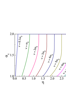
Figure 3: (Color online) Critical value of the exponent of the confinement frequency as a function of the density for different values of the strength of the confinement potential. We took the parameters $n=1$ and $\kappa=1$

Finally we may find analytical expressions for the order parameter from Eq. (28) for different values of $\alpha\geq 2$, which are given in Table 3. Notice that it is always possible to find a $\psi\neq 0$ which indicates that the single chain configuration is always unstable when $\alpha>2$. For $\alpha=2$ we find $\psi\neq 0$ only when $\tilde{a}(n,\tilde{\kappa})<1$.

Table 3: Order parameter for different values of $\alpha$.

$\alpha$	$\psi$
2	$\sqrt{(1-\tilde{a})/\tilde{b}}$
3	$\left(-\tilde{a}+\sqrt{\tilde{a}^{2}+4\tilde{b}}\right)/2\tilde{b}$
4	$1/\sqrt{\tilde{a}+\tilde{b}}$

III Results and discussion

As has been found in previous section, a continuous zig-zag transition occurs for parabolic confinement. For the case ($\alpha\neq 2$) it is not possible to define a transition between the one-chain and two-chain configuration, because the confinement potential does not contribute to the second order term of the total potential energy. Additionally we find that the minimum value of the transverse frequency is purely imaginary, see Eqs. (15a) and (16a), and this condition implies that in this case the transition for the one-chain to the two-chains configuration is not allowed which agrees with previous006_piacente results. We also performed Monte-Carlo simulations and found that for $\alpha>2$ the one-chain configuration is never formed for any value of the density and the confinement frequency. However from similar simulations one can show that for $\alpha<2$ the one-chain configuration is stable until a critical point, beyond which the configuration is changed to a single chain containing vacancies due to jumps of individual particles away from the chain axis.

III.1 Transition point for $\alpha\leq 2$

For the case of a power-law inter-particle potential ($\kappa=0$) with parabolic confinement and using dimensionless units, it is possible to find an analytical relationship between the confinement frequency and the linear density as $\eta=\upsilon^{-2/(n+2)}$. For this case we show in Fig. 4 the behavior of the order parameter as a function of the linear density for different values of $n$. Dashed curves represent the solution from the Landau theory, Eq. (6), the full curves are the solution of Eq. (21) and they are compared with the results of a Monte-Carlo simulation for $n=1$ and $n=3$ (open circles in Fig. 4). From these results we notice that there is perfect agreement between our calculation and the exact results obtained from Monte-Carlo simulations. In the same context Fig. 5 shows the variation of the critical density as a function of the exponent $n$ as obtained from Landau theory (solid and dashed curves for $\kappa=0$ and $\kappa=1$, respectively) and the result from the present work (full and open circles for $\kappa=0$ and $\kappa=1$) the results are shown for different confinement frequencies. Notice that for $\upsilon=1$ this function has a local minimum where the dipole potential exhibits the lowest critical density.

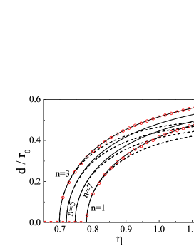
Figure 4: (Color online) Displacement from the $x$-axis as a function of the linear density for $\upsilon=1$. The dashed lines are obtained from the Landau theory while the solid lines are the solutions of Eq. (21). The open circles represent the results of our Monte-Carlo simulations for $n=1$ and $n=3$

.

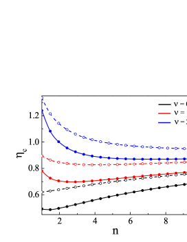
Figure 5: (Color online) Critical linear density as a function of the $n$ exponent of the inter-particle interaction for different values of the parabolic confinement frequency. The (solid and dashed) lines are the prediction of the Landau theory and the (solid and open) circles are found with the present method (for $\kappa=0$ and $\kappa=1$ respectively).

On the other hand, it is also possible to find the value of $d$ numerically by fixing one particle at a distance $y$ from the one-chain axis in the confinement direction and minimise the energy with respect to the position of the other particles. The resulting minimum potential energy of the system is shown in Fig. 6 for a Yukawa inter-particle potential with $\kappa=1$ and $\upsilon=1$. For $\eta\leq\eta_{c}$ the minimum is found at $y=0$ and for $\eta>\eta_{c}$ it continuously shifts to $y\neq 0$, which is typical for a second order transition.

Figure 6: Potential energy per particle as a function of the position of one of the particles in the confinement direction, before ($\eta=0.78\eta_{c}$), after ($\eta=1.34\eta_{c}$) and at the transition ($\eta=\eta_{c}$) for parabolic confinement. We took the parameters $\upsilon=1$, $\kappa=1$ and $n=1$

From Eq. (19) we draw the contour plot of $\upsilon_{c}$ as a function of $n$ and $\kappa$ for several values of the density (when making the contour plot we replaced $n$ by a real number), which are shown in Fig. 7. We observe a strong dependence of the highest value of $\upsilon_{c}$ on $\eta$, and therefore the region of frequencies over which the one-chain configuration exists. For low densities ($\eta<1$) the one-chain organization is dominant for small values of the exponent $n$ and gradually this region is extended to higher values of $n$ with increasing $\eta$. This result shows that for low densities the one-dimensional behavior of the system is a better representation for the Coulomb and dipole inter-particle potential. For $\eta\geq 1$ the one-dimensional region of frequencies increasing with increasing $n$. In all cases the critical frequency decreases with increasing $\kappa$.

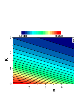
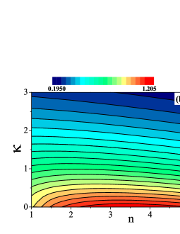
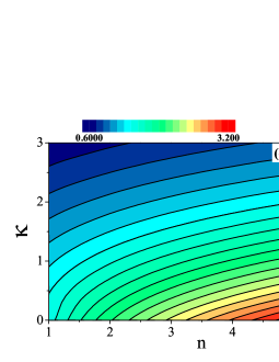
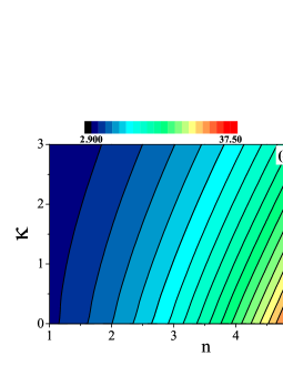
Figure 7: (Color online) Contour plots of the critical frequency $\upsilon_{c}$ as a function of $n$ and $\kappa$, for (a) $\eta=0.50$, (b) $\eta=0.75$, (c) $\eta=1.00$, (d) $\eta=2.00$, in case of a parabolic confinement potential.

first

Our previous mean-field theory was derived for modes of the linear chain close to the instability point. Therefore, it is possible to find the critical point for the aforementioned instability from Eq. (27). In Fig. 8 we plot the transition point at which the one-chain structure becomes unstable for $\alpha\leq 2$. Above each curve only $\psi=0$ is a solution of Eq. (27). Only for $\alpha=2$ the curves corresponds to a second order zig-zag transition. Notice that the stability region for the single chain configuration increases with decreasing $\alpha$.

Figure 8: Critical transition point for the one-chain configuration. Above the curves the one chain configuration is the ground state. Results are shown for (a) Coulomb potential, (b) dipole potential and (c) Yukawa potential, for different values of the exponent of the confinement potential $\alpha$.

In Fig. 9(a) we show the dispersion relation for the normal modes in the case of parabolic confinement for different values of $\kappa$ in the three cases, linear regime (dotted lines) where the system is stable for any value of the wavevector close to $k_{0}$, the zig-zag regime (dashed lines), and in the transition point (solid lines) where the dispersion is linear close to $k_{0}$.

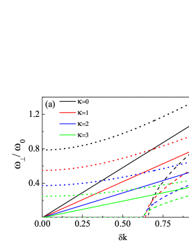
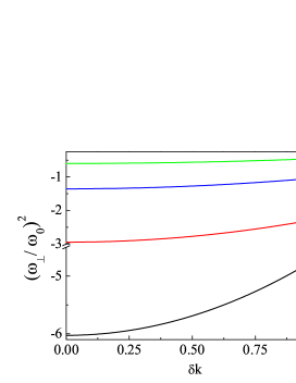
Figure 9: (Color online) (a) Dispersion relation $\omega_{\perp}$ as a function of $\delta k$ for parabolic confinement (i.e. $\alpha=2$) where dashed, solid and dotted lines represent the results for $\upsilon=0.95\upsilon_{c}$, $\upsilon=\upsilon_{c}$ and $\upsilon=1.05\upsilon_{c}$ respectively. (b) Square transverse frequency $\omega_{\perp}^{2}$ as a function of $\delta k$ for $\alpha>2$. We have considered $n=1$, $\eta=1$ and different values of $\kappa$ as shown in (a).

III.2 Case $\alpha>2$

In this case the most simple configuration of the particles is restricted to a 2-chains structure, however from Monte-Carlo simulations we know that there is a transition to a 4-chains structure after some value of the linear density. This is shown in Fig. 10, where we plot the distance from the $y=0$ axis of the particles as a function of the density considering a dipole inter-particle interaction for different values of $\alpha$. In those figures the 2-chains to 4-chains transition point is marked with a vertical dashed line. In our theoretical model we have found from Eqs. (15a) and (16a) that $\omega_{\perp}^{2}<0$ as shown in Fig. 9(b) and thus the transverse frequency is imaginary and therefore the one-chain structure is unstable for any value of the density and the confinement strength.

Figure 10: Distance of the particles from the $y$-axis as a function of the density, for different values of $\alpha$ and $\upsilon=1$. The inter-particle interaction is a dipole potential. The symbols represent the results from Monte-Carlo simulations and the dashed vertical lines indicate the transition point from the 2-chains to the 4-chains configuration.

This is illustrated in more detail in Fig. 11 where we plot the distance of the particles from the $x$-axis for different values of $\eta$. Note that our mean-field results from Eq. (27) agree with the simulation for small values of $\eta$. Note that for small values the confinement potential energy is significantly larger than the inter-particle potential energy and therefore the fluctuations of the order parameter are smaller. With increasing $\eta$ the interaction between the particles start to dominant and all curves converge to each other (without crossing) for $\eta>1$.

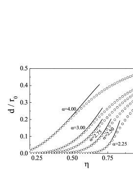
Figure 11: Order parameter as a function of the linear density in the 2-chains region for different values of the exponent of the confinement potential $\alpha$. The solid curves represent the solutions of Eq. (27) and open circles the results of our Monte-Carlo simulation. We took the parameters $\upsilon=1$, $\kappa=1$ and $n=1$.

IV Conclusions

In this work, we studied the critical behavior of a system of particles confined in a 2D channel through a $y^{\alpha}$ potential with different functional forms for the inter-particle interaction potential. We derived a Ginzburg-Landau equation for the system and determine the behavior of the system close to the transition point where the single chain configuration becomes unstable. We determined the order parameter and its dependence on the external confinement and the particle density.

For $\alpha=2$ the critical frequency for the zig-zag transition is larger than for smaller values of $\alpha$, which shows that the stability of the linear chain configuration is lower for parabolic confinement. However for low densities ($\eta<1$) the one-chain configuration is the most stable state for $\alpha\leq 2$.

For $\alpha>2$ the single chain configuration is unstable for any value of the particle density and the strength of the confinement potential. We found the distance between the two chains as function of the particle density. With increasing density a first-order phase transition is found to the 4-chains configuration.

For $\alpha<2$ we found analytically no continuous zig-zag configuration irrespective of the inter-particle potential. The instability of the single chain configuration occurs through the expulsion of single particles from the chain to $y\neq 0$ positions.

The instability point for $\alpha=2$ is given by $\upsilon_{c}=\eta_{c}^{2/(n+2)}$ which becomes an almost linear relation, i.e. $\upsilon_{c}\sim\eta_{c}$ for $\alpha=1$ and $n=1$.

In a future work we plan to generalize the present analysis to the quantum regime. for the special case of electrons confined by a parabolic potential, i.e. $\alpha=2$, $n=1$ and $\lambda=\infty$, such an analysis was presented by J. S. Meyer et. al. 038_Meyer ; 039_Meng . Subsequently the strongly correlated regime which results in Wigner crystal physics in quantum wires, was addressed in Ref. [040_Meyer, ]. Such a quantum analysis will address the effect of quantum statistics of the particles and the effect of quantum fluctuations on the zig-zag transition.

V Acknowledgments

This work was supported by the Flemish Science Foundation (FWO-Vl).

References

- (1) H. Ikegami, H. Akimoto, and K. Kono, Phys. Rev. Lett. 102, 046807 (2009)
- (2) W. M. Itano, J. J. Bollinger, J. N. Tan, B. Jelenkovic, X.-P. Huang, and D. J. Wineland, Science 279, 686 (1998)
- (3) I. Waki, S. Kassner, G. Birkl, and H. Walther, Phys. Rev. Lett. 68, 2007 (1992)
- (4) D. H. E. Dubin and T. M. O’Neil, Rev. Mod. Phys. 71, 87 (1999)
- (5) A. Mortensen, E. Nielsen, T. Matthey, and M. Drewsen, Phys. Rev. Lett. 96, 103001 (2006)
- (6) J. I. Cirac and P. Zoller, Phys. Rev. Lett. 74, 4091 (1995)
- (7) D. Leibfried, B. DeMarco, V. Meyer, D. Lucas, M. Barret, J. Britton, W. M. Itano, B. Jelenkovic, C. Langer, T. Rosenband, and D. J. Wineland, Nature 422, 412 (2003)
- (8) J. M. Taylor and T. Calarco, Phys. Rev. A. 78, 062331 (2008)
- (9) Y. G. Cornelissens, B. Partoens, and F. M. Peeters, Physica E 8, 314 (2000)
- (10) R. W. Hasse and V. V. Avilov, Phys. Rev. A 44, 4506 (1991)
- (11) I. V. Schweigert, V. A. Schweigert, and F. M. Peeters, Phys. Rev. B 54, 10827 (1996)
- (12) V. A. Schweigert and F. M. Peeters, Phys. Rev. B 51, 7700 (1995)
- (13) B. Partoens, V. A. Schweigert, and F. M. Peeters, Phys. Rev. Lett. 79, 3990 (1997)
- (14) G. Piacente, I. V. Schweigert, J. J. Betouras, and F. M. Peeters, Phys. Rev. B 69, 045324 (2004)
- (15) S. Fishman, G. DeChiara, T. Calarco, and G. Morigi, Phys. Rev. B 77, 064111 (2008)
- (16) W. Yang, M. Kong, M. V. Milosevic, Z. Zeng, and F. M. Peeters, Phys. Rev. E 76, 041404 (2007)
- (17) A. Valkering, J. Klier, and P. Leiderer, Physica B 284, 172 (2000)
- (18) T. Y. M. Chan and S. John, Phys. Rev. A. 78, 033812 (2008)
- (19) C. Lutz, M. Kollmann, P. Leiderer, and C. Bechinger, J. Phys.: Condens. Matter 16, S4075 (2004)
- (20) C. Lutz, M. Kollmann, and C. Bechinger, Phys. Rev. Lett. 93, 026001 (2004)
- (21) D. Lucena, D. V. Tkachenko, K. Nelissen, V. R. Misko, W. P. Ferreira, G. A. Farias, and F. M. Peeters, preprint cond-mat/1010.4540v1(2010)
- (22) J. B. Delfau, C. Coste, and M. S. Jean, preprint cond-mat/1103.3642v1(2011)
- (23) G. Piacente, G. Q. Hai, and F. M. Peeters, Phys. Rev. B 81, 024108 (2010)
- (24) A. del Campo, G. D. Chiara, G. Morigi, M. B. Plenio, and A. Retzker, New J. Phys. 12, 115003 (2010)
- (25) T. E. Sheridan and A. L. Magyar, Phys. Plasmas 17, 113703 (2010)
- (26) T. L. L. Closson and M. R. Roussel, Can. J. Chem. 87, 1425 (2009)
- (27) T. E. Sheridan and K. D. Wells, Phys. Rev. E 81, 016404 (2010)
- (28) K. Yosida, Functional Analysis, 3rd ed. (Springer, Berlin, 1971) pp. 153–154
- (29) L. D. Landau and E. M. Lifshitz, Statistical Physics, 3rd ed. (Pergamon Press, New York, 1986) pp. 179–181
- (30) J. S. Meyer, K. A. Matveev, and A. I. Larkin, Phys. Rev. Lett. 98, 126404 (2007)
- (31) T. Meng, M. Dixit, M. Garst, and J. S. Meyer, Phys. Rev. B 83, 125323 (2011)
- (32) J. S. Meyer and K. A. Matveev, J. Phys.: Condens. Matter 21, 023203 (2009)