Structural transitions in vertically and horizontally coupled parabolic channels of Wigner crystals

Abstract

Structural phase transitions in two vertically or horizontally coupled channels of strongly interacting particles are investigated. The particles are free to move in the $x$-direction but are confined by a parabolic potential in the $y$-direction. They interact with each other through a screened power-law potential ($r^{-n}e^{-r/\lambda}$). In vertically coupled systems the channels are stacked above each other in the direction perpendicular to the $(x,y)$-plane, while in horizontally coupled systems both channels are aligned in the confinement direction. Using Monte Carlo (MC) simulations we obtain the ground state configurations and the structural transitions as a function of the linear particle density and the separation between the channels. At zero temperature the vertically coupled system exhibits a rich phase diagram with continuous and discontinuous transitions. On the other hand the vertically coupled system exhibits only a very limited number of phase transitions due to its symmetry. Further we calculated the normal modes for the Wigner crystals in both cases. From MC simulations we found that in the case of vertically coupled systems the zigzag transition is only possible for low densities. A Ginzburg-Landau theory for the zigzag transition is presented, which predicts correctly the behavior of this transition from which we interpret the structural phase transition of the Wigner crystal through the reduction of the Brillouin zone.

I Introduction

Self-organized systems are of fundamental importance in different areas of physics. can be seen in the accelerated progress in that area. It all started in 1934 when Wigner045_wigner surmised that, if considering an electron gas, where the electrons have no kinetic energy, as occurs in low density systems, then these electrons “would settle in configurations which correspond to the absolute minima of the potential energy. These are closed-packed lattice configurations, with energies very near to that of the body-centered lattice.” This was the first prediction about self-organized systems of electrons and charged particles, which today is known as Wigner crystals.

At the present it is known that Wigner crystals form a body-centered cubic (BCC) lattice in three-dimensional008_hasse ; 005_cornelissens (3D) space, a triangular lattice in two-dimensional004_schweigert ; 009_partoens (2D) systems, while in one-dimensional (1D) systems, the energetically more favorable array is given by an evenly spaced lattice. Wigner crystals have been the study object of several experiments020_itano ; 021_waki ; 022_ikegami ; 023_mortensen ; 033_dubin and theoretical works 006_piacente ; 014_fishman ; 001_kwinten ; 002_kwinten ; 003_kwinten ; 004_kwinten in recent years.

Recently, the transition between 1D and 2D systems has been analyzed, known as quasi-one-dimensional (Q1D) systems. Several studies003_piacente ; 006_piacente have investigated different properties of the Wigner crystal in that regime. When increasing the density, the linear chain structure undergoes a zigzag transition that occurs always through a continuous transition. This zigzag transition has been observed in different experiments029_lutz ; 031_chan and analyzed in different systems: colloidal systems027_saintjean ; 005_kwinten ; 006_kwinten ; 007_kwinten ; 008_kwinten , vortices in superconductor/ferromagnetic hybrids043_karapetrov . They have also been proposed as a possible implementation of a quantum information processor026_leibfried .

The zigzag transition for a system of Coulomb particles subjected to a parabolic confinement potential011_delcampo was analyzed through a Ginzburg-Landau theory. Later this theory was applied to more complex particle interactions and generalized for a power-law confining potential041_galvan . In the latter work it was shown that this theory leads to a better representation of the phase transition behavior close to the critical point.

In the present work we analyze the phase transitions between two vertically and horizontally coupled Q1D channels as function of the inter-channel distance and linear particle density in each channel. Further the zigzag transition of the vertically coupled channels is compared with the analytical results obtained from the Ginzburg-Landau approach.

The present paper is organized as follows. In Sect. II the model system is formulated. In Sect. III the numerical results are presented with an analysis about the behavior of the system in the different structural phases. In Sect. IV the Ginzburg-Landau Lagrangian is derived and the theoretical results are discussed and compared with our numerical simulations. Our conclusions are given in Sect. V.

II Model system

In this work we consider a system consisting of two quasi-one-dimensional channels each with $N$ identical particles with mass $m$ and charge $q$, which are restricted to move in the $(x,y)$-plane. The system is subjected to an external magnetic field $\mathbf{B}$, which is applied in the direction perpendicular to the channels. The particles are confined by a one-dimensional potential limiting their motion in the $y$-direction in each channel. The channels are separated by a distance $d_{y}$ from each other in the $y$-direction and a distance $d_{z}$ in the $z$-direction as shown in Fig. 1.

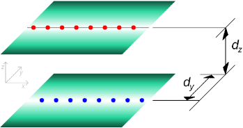
Figure 1: (Color online) Schematic representation of the model system, where the filled circles represent the particles in each channel, $d_{y}$ and $d_{z}$ indicate the distance between the channels in the $y$- and $z$- axis respectively. The darker colors in each plane represent the increases of the strength of the confinement potential in the channel.

The charged particles interact through a repulsive interaction potential. The kinetic energy of the system is given by:

$$T=\sum_{i=1}^{N}{\frac{\mathbf{p}_{1i}^{2}}{2m}}+\sum_{i=1}^{N}{\frac{\mathbf{p}_{2i}^{2}}{2m}},$$ (1)

where $\mathbf{p}_{ki}=m\mathbf{v}_{ki}+q\mathbf{A}_{ki}$ represents the canonical momentum of particle $i$ in channel $k$, which is moving with velocity $\mathbf{v}_{ki}$. $\mathbf{A}_{ki}$ is the vector potential related to the magnetic field through the relation $\mathbf{B}=\nabla\times\mathbf{A}_{ki}$. The total energy of the system is given by:

$$E = \frac{m}{2}\sum_{i=1}^{N}(\dot{\mathbf{r}}_{1i}^{2}+\dot{\mathbf{r}}_{2i}^{2})+q\sum_{i=1}^{N}(\dot{\mathbf{r}}_{1i}\cdot\mathbf{A}_{1i}+\dot{\mathbf{r}}_{2i}\cdot\mathbf{A}_{2i})$$ (2)

$$+\frac{q}{2m}\sum_{i=1}^{N}(\mathbf{A}_{1i}^{2}+\mathbf{A}_{2i}^{2})+V_{conf}+V_{int},$$

where the confinement and the interaction potential are, respectively, given by:

$$V_{conf}=\frac{1}{2}m\upsilon_{t}^{2}\sum_{i=1}^{N}\left(y_{1i}-\frac{d_{y}}{2}\right)^{2}+\frac{1}{2}m\upsilon_{t}^{2}\sum_{i=1}^{N}\left(y_{2i}+\frac{d_{y}}{2}\right)^{2},$$ (3a)

$$V_{int} = \sum_{i=1}^{N}\sum_{j>i}^{N}V_{pair}(r_{1i,1j})+\sum_{i=1}^{N}\sum_{j>i}^{N}V_{pair}(r_{2i,2j})$$ (3b)

$$+\sum_{i=1}^{N}\sum_{j=1}^{N}V_{pair}(r_{1i,2j}).$$

Here, $V_{pair}(r)$ represents the inter-particle potential which is taken as a screened power-law potential, which will allow for the simulations of both long- and short-range interactions, as follows:

$$V_{pair}(r)=\frac{q^{2}}{\epsilon R}\frac{R^{n}e^{-r/\lambda}}{r^{n}}.$$ (4)

In general $r_{Ai,Bj}=|\mathbf{r}_{Ai}-\mathbf{r}_{Bj}|$ represents the relative position between the $i$-th particle in channel $A$ and the $j$-th particle in channel $B$. The exponent $n$ is an integer and $\epsilon$ is the dielectric constant of the medium where the particles are moving in. In the above, $R$ is an arbitrary length parameter which we introduced to guarantee the correct units. The magnetic field is taken to be constant and is applied in the direction perpendicular to the plane formed by the channels, through the vector potential defined by $\mathbf{A}_{ki}=-By_{ki}\mathbf{e_{x}}$. The total energy can be written in dimensionless form as follows:

$$E = \sum_{i=1}^{N}(\dot{\mathbf{r}}_{1i}^{2}+\dot{\mathbf{r}}_{2i}^{2})-B\sum_{i=1}^{N}(\dot{x}_{1i}y_{1i}+\dot{x}_{2i}y_{2i})$$ (5)

$$+\left(\upsilon^{2}+\frac{B^{2}}{4}\right)\sum_{i=1}^{N}(y_{1i}^{2}+y_{2i}^{2})$$

$$+d_{y}\upsilon^{2}\sum_{i=1}^{N}\left(y_{1i}-y_{2i}-\frac{d_{y}}{2}\right)$$

$$+\sum_{i=1}^{N}\sum_{j>i}^{N}\frac{e^{-\kappa r_{1i,1j}}}{r_{1i,1j}^{n}}+\sum_{i=1}^{N}\sum_{j>i}^{N}\frac{e^{-\kappa r_{2i,2j}}}{r_{2i,2j}^{n}}$$

$$+\sum_{i=1}^{N}\sum_{j=1}^{N}\frac{e^{-\kappa r_{1i,2j}}}{r_{1i,2j}^{n}},$$

where the dimensionless frequency is given by $\upsilon=\upsilon_{t}/\omega_{0}$, while $\omega_{0}$ measures the strength of the confinement potential and $t_{0}=1/\omega_{0}$ is the unit of time. The unit of the energy is given by: $E_{0}=\left(m\omega_{0}^{2}/2\right)^{n/(n+2)}\left(q^{2}/\epsilon\right)^{2/(n+2)}R^{2(n-1)/(n+2)}$, the distances are scaled with $r_{0}=\left(2q^{2}/m\omega_{0}^{2}\epsilon\right)^{1/(n+2)}R^{(n-1)/(n+2)}$, and the strengths of the magnetic field and the vector potential are measured in units of $B_{0}=2m\omega_{0}/q$ and $A_{0}=B_{0}r_{0}$, respectively. Additionally, the dimensionless parameter $\kappa=r_{0}/\lambda$ represents the screening parameter of the potential. In order to describe better the behavior of the transitions in the system, we define a dimensionless linear density $\eta$ as the number of particles per unit of length along the unconfined direction in each channel. This density is chosen to be equal in both channels.

III Numerical Model

In order to understand the behavior of coupled systems, we consider two different cases. Case A corresponds to two vertically coupled channels where the distance between the channels in the $y$-direction is taken zero. In this case the channels are arranged above each other. Case B consists of two horizontally coupled channels with $d_{z}=0$, which are aligned parallel to each other separated by a distance $d_{y}$. In order to find the ground state configuration for each case we have performed Monte Carlo simulations, complemented with the Newton optimization technique004_schweigert ; 002_schweigert . Using those methods we construct the phase diagram of the ground state configuration of the system at zero temperature as a function of the separation between the two channels and the linear density.

III.1 Case A: Vertical Coupling

The phase diagram of vertically coupled channels is shown in Fig. 2 for an interaction potential with parameters $n=1$ and $\kappa=1$ and fixed value of the frequency $\upsilon=1$. The phases are represented by the number in each delimited region, the solid lines represent first order transitions and the dashed lines second order transitions.

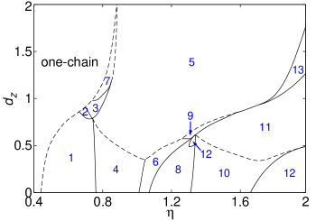
Figure 2: Phase diagram of vertically coupled channels as a function of the linear particle density and the distance between the channels in the $z$-direction. Solid and dashed lines represent first and second order transitions, respectively. The different phases are discussed in the text and shown in Fig. 3.

From this phase diagram we see that the zigzag transition occurs only between the one-chain configuration and phase $1$ where particles of each channel are organized in a single chain, this transition is continuous and of second order. The different phases are shown in Fig. 3. One can see that the activation point, defined as the point where the one-chain arrangement is no longer the only possible ground state configuration for any value of $d_{z}$, is given by $\eta_{act}=0.447302$ for $d_{z}=0$. This value of the linear density represents exactly half the value of the critical density ($\eta_{c}$) for the zigzag transition in the case of a single Q1D channel as was found in Refs. 006_piacente, ; 041_galvan, . Notice that for increasing $d_{z}$, the critical density increases as well, which means a change in the total dimensionality of the system. Additionally, one can observe that for $d_{z}>0.5$, $\eta_{c}$ increases more quickly than for $d_{z}<0.5$. This implies that the system tends to behave as two decoupled channels, until the point where the zigzag transition disappears.

The different ground state configurations identified in Fig. 2 are shown in Fig. 3. In this figure, the red filled circles represent the particles in channel A and the blue open circles the particles in channel B. The gray arrows between two configurations indicate that the transition between them occurs continuously, following the process described through the small black arrows inside each phase configuration. The small black arrows above each particle represent the displacement direction when the separation between the channels is increased. It is interesting to observe that the phases $7$, $8$ and $13$ are composed of several configurations whose transition occurs through a continuous phase transition indicated by the small black arrows plotted inside the pictures.

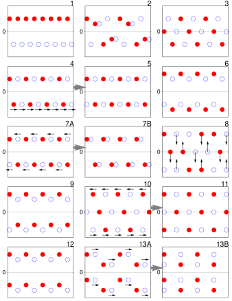
Figure 3: (Color online) Configurations of the different crystalline phases of the particles as enumerated in the phase diagram presented in Fig. 2. The red solid (blue open) symbols are the particles in the top (bottom) channel.

The eigenvectors of the first non-zero eigenfrequency for each ground state configuration is shown in Fig. 4. The direction of the eigenvector is of particular interest because it contains information about the onset of melting in that crystal, when temperature is increased.

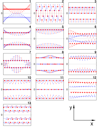
Figure 4: (Color online) Eigenvectors of the first non-zero frequency of each phase for vertically coupled systems.

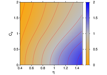
Figure 5: (Color online) Contour plots of the energy per particle as a function of the linear density $\eta$ in each channel and the vertical separation $d_{z}$ between the channels. The red lines represent the iso-energy lines of the system.

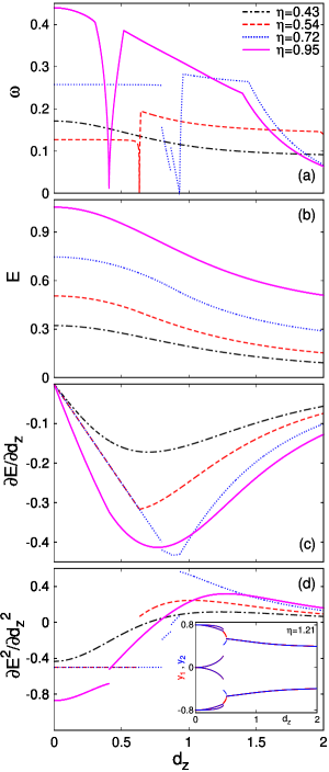
Figure 6: (Color online) (a) First non-zero eigenfrequency; (b) Energy per particle; (c) First derivative of the energy; (d) Second derivative of the energy. In all figures we have plotted as a function of the vertical separation between the channels. The colors showed at the top represent the different densities. The inset in (d) shows the distance of the chains from the $x$-axis of the channels as a function of the vertical separation for $\eta=1.21$.

In order to know the evolution of the system it is interesting to show the behavior of the total energy as a function of the control parameter. This can be seen in Fig. 5, where the contour plots of the energy per particle are plotted as a function of the linear density and the vertical separation between channels. The color scale indicates the magnitude of the energy and the lines show the iso-energy lines on the plot. Notice that by increasing the density, the iso-energy lines become increasingly curved showing the decoupling of the channels, due to the increase of the interaction between particles in the same channel, while the energy contribution from the interaction between channels becomes significantly smaller with increasing $d_{z}$.

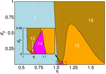
Figure 7: (Color online) Phase diagram of the system as a function of the linear density ($\eta$) and the distance between the channels in $y$-direction ($d_{y}$). All phase transitions are first order transitions.

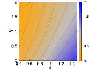
Figure 8: (Color online) Contour plots of the energy per particle as a function of the linear density $\eta$ in each channel and the horizontal separation $d_{y}$ between channels. The red lines represent the iso-energy lines of the system.

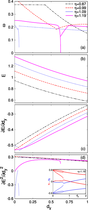
Figure 9: (Color online) (a) First non-zero eigenfrequency; (b) Energy per particle; (c) First derivative of the energy; (d) Second derivative of the energy. All figures are plotted as a function of the horizontal distance between the channels. The colors showed at the top represent the different densities. The inset in (d) shows the distance of the chains from the center of each channel as a function of the horizontal separation for $\eta=1.19$.

With the aim to explain the order of the transitions, we plot in Fig. 6 the first non-zero eigenfrequency for different densities. We also plot the energy per particle and its two first derivatives with respect to the vertical separation. In all cases the figures show the behavior of these quantities as a function of the separation between channels, and the value of the density taken for each curve is printed at the top of the figure. From the smooth and monotonic behavior of the energy in Fig. 6(b) and the jumps in its derivatives (see Figs. 6(c,d)), we can deduce the order of each phase transition, which following the Ehrenfest classification B03_Uzunov are given by the order of the lowest derivative of the energy which exhibits a discontinuity. From Fig. 6(a) we note that the transitions between phase 1 and phase 2 (shown for $\eta=0.72$ around $d_{z}=0.798$) and between phase 2 and phase 3 (shown for $\eta=0.72$ around $d_{z}=0.866$) are of first order which can be seen by the jumps in the first derivative of the energy at the transition points. The transitions of second order are characterized by the softening of an eigenmode, i.e. $\omega=0$. The inset in Fig. 6(d) shows the $y$-position of each chain for $\eta=1.21$, where one can see the continuous transition from $3$ to $6$ chains, the first order transition between $6$ and $4$ chains and the second and continuous transitions between $4$ and $2$ chains. The red and blue lines represent the positions of the particles in channel A and channel B.

III.2 Case B: Horizontal Coupling

In this part we analyze horizontally coupled channels ($d_{z}=0$) for the same parameters as in case A. The phase diagram in this case is shown in Fig. 7 as a function of the linear density $\eta$ and the vertical separation between the channels $d_{y}$.

From this phase diagram we notice that the zigzag transition does not occur in horizontally coupled channels. The one-chain configuration only exists when $d_{y}=0$ and for $\eta<\eta_{act}$. Additionally the small number of phases is a result of the weaker interaction between channels.

In Fig. 8 we show a contour plot of the energy per particle and iso-energy lines as a function of the linear density and the horizontal separation between the channels. Notice the smooth and monotonic behavior of the iso-energy lines, which align parallel to each other with increasing linear density. When increasing $d_{y}$, the interaction between the channels decreases quickly due to the separation between channels which is directly related with the confinement potential as can be seen in Eq. (5), where $d_{y}$ contributes to the total energy of the system introducing a linear term of the relative position between particles in the $y$-direction. This contribution leads to the disappearance of the harmonicity of the system.

In Fig. 9(a) we show the first non-zero frequency as a function of the horizontal separation for different densities, which shows clearly the phase transition points. The monotonic and continuous behavior of the energy (Fig. 9(b)) and the jumps in the first derivative of the energy, as shown in Fig. 9(c), indicates, that all phase transitions are of first order. In those transition points we also can see that the first non-zero eigenfrequency has a jump, which shows the abrupt change in the vibration mode of the system in the phase transitions. As an illustration about the first order transitions in the system, we show in the inset of Fig. 9(d) the $y$-distance of the chains from the center of each channel, where one can see the transitions between $3$, $8$ and $4$ chains for $\eta=1.19$. In this figure the red and blue lines represent the particles in channel A and channel B, respectively.

The different configurations of the phases shown in the phase diagram of the horizontally coupled system, are plotted in Fig. 10(a), where the gray arrows and the small black arrows have the same meaning as previously. Notice that phases $14$ and $15$ consist of several phases. The transition between those phases occurs through continuous transitions. In Fig. 10(b) the normal mode of the first non-zero frequency is plotted for each configuration.

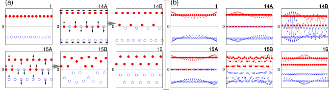
Figure 10: (Color online) (a) Configurations of the crystalline organization of particles enumerated in the phase diagram presented in Fig. 7. (b) Eigenvector of the first non-zero frequency of each phase configuration.

IV Ginzburg-Landau Model for linear-zigzag transition

The results of previous section indicates that the transition between the one-chain arrangement and the zigzag configuration occurs in the low density region and only in the case of a vertically coupled system. To analyze this transition (i.e. $d_{y}=0$), we start by considering the system in the situation that the one-chain configuration is stable in each channel and close to the zigzag transition point. The equilibrium positions of all particles are given by $\mathbf{r}_{ki}^{lin}=(x_{ki}^{lin},0,(k-1)d_{z})$ with $x_{ki}^{lin}=[2i+(2-k)]/2\eta$, where $k$ represents the channel number (i.e. $1$ or $2$) and $i$ the particle number in that channel. Further we consider small oscillations around the equilibrium positions in the $y$-direction. The position of each particle becomes thus $\mathbf{r}_{ki}=\mathbf{r}_{ki}^{lin}+\Delta\mathbf{r}_{ki}$, where the small displacements are given by $\Delta\mathbf{r}_{ki}=(0,y_{ki},0)$. Now, ensuring that the particles are oscillating around these ground state positions, and assuming that these oscillations are much smaller than the distance between the two nearest particles, we expand $r_{1i,2j}$ into a power series.

As found numerically, this transition is continuous and the configuration after the transition point consists of a zigzag configuration (phase $1$ in Fig. 2), but with all particles forming a single off-center chain in each channel (i.e. $y_{1i}=c$ and $y_{2i}=-c$, with $c$ as a real number). From that configuration we can observe that there is a competition between the interaction potentials $V_{11}$, $V_{22}$ and $V_{12}$ which are defined as the last three terms in Eq. (5) respectively. The subindexes represent the interacting channels. The first two interaction potentials ($V_{11}$, $V_{22}$) do not contribute to the solution in this case, since all particles in the same channel are aligned parallel to the $x$-axis. Thus, the interaction between the particles in the different channels, as well as the confinement potential, are responsible for this transition.

Following Ref. 041_galvan, , we obtain the Lagrangian density of the system in the continuum limit by considering only the interaction potential $V_{12}$:

$$\mathcal{L}=\frac{1}{2} \Big{[} h^{2}(n,\tilde{\kappa},c_{z})(\partial_{x}\psi(x))^{2}+\delta_{\upsilon}(n,\tilde{\kappa},c_{z})\psi^{2}(x)$$ (6)

$$+\mathcal{A}(n,\tilde{\kappa},c_{z})\psi^{4}(x)\Big{]},$$

where $\tilde{\kappa}=\kappa/\eta$, $c_{z}=\eta d_{z}$, $\delta_{\upsilon}(n,\tilde{\kappa},c_{z})=2(\upsilon^{2}+B^{2}/4)-\varpi^{2}(n,\tilde{\kappa},c_{z})$ and the order parameter $\psi(x)$ represents the separation between channels (i.e. $\psi=2c$). The coefficients are given by:

$$h^{2}(n,\tilde{\kappa},c_{z}) = \eta^{n}\Bigg{[}n\sum_{j=0}^{\infty}\frac{e^{-\tilde{\kappa}R_{j}}}{R_{j}^{n}}\left(1-2\sin^{2}\left(\frac{R_{j}\tilde{k}_{0}}{2}\right)\right)+\tilde{\kappa}\sum_{j=0}^{\infty}\frac{e^{-\tilde{\kappa}R_{j}}}{R_{j}^{n-1}}\left(1-2\sin^{2}\left(\frac{R_{j}\tilde{k}_{0}}{2}\right)\right)\Bigg{]}$$ (7)

$$\varpi^{2}(n,\tilde{\kappa},c_{z}) = 4\eta^{n+2}\Bigg{[}n\sum_{j=0}^{\infty}\frac{e^{-\tilde{\kappa}R_{j}}}{R_{j}^{n+2}}\sin^{2}\left(\frac{R_{j}\tilde{k}_{0}}{2}\right)+\tilde{\kappa}\sum_{j=0}^{\infty}\frac{e^{-\tilde{\kappa}R_{j}}}{R_{j}^{n+1}}\sin^{2}\left(\frac{R_{j}\tilde{k}_{0}}{2}\right)\Bigg{]}$$ (8)

$$\mathcal{A}(n,\tilde{\kappa},c_{z}) = 2n\eta^{n+4}\Bigg{[}\frac{n+2}{2}\sum_{j=0}^{\infty}\frac{e^{-\tilde{\kappa}R_{j}}}{R_{j}^{n+4}}\sin^{4}\left(\frac{R_{j}\tilde{k}_{0}}{2}\right)+\tilde{\kappa}\sum_{j=0}^{\infty}\frac{e^{-\tilde{\kappa}R_{j}}}{R_{j}^{n+3}}\sin^{4}\left(\frac{R_{j}\tilde{k}_{0}}{2}\right)\Bigg{]},$$ (9)

where $R_{j}=\sqrt{(j+1/2)^{2}+c_{z}^{2}}$ and $\tilde{k}_{0}=k_{0}/\eta$ represent the value of the wavevector in the stability point.

IV.1 Stability Point

The stability point is calculated numerically, as the location of the minimum of the second order term of the total energy, and the value of the wavevector is called $k_{0}$. Then the stability point is found from the condition $\min\delta_{\upsilon}(n,\tilde{\kappa},c_{z})$. Notice that the value of $\tilde{k}_{0}$ depends on the distance between channels. For $c_{z}=0$ we can find analytically that $\tilde{k}_{0}=2\pi$, which implies that the particle density ($\eta$) of the system in each channel will be reduced to half of the density required to find the stability point in one channel as found previously006_piacente ; 041_galvan . Next, from the stability condition we find for $\upsilon=1$ that the activation point (minimum value of density to find the zigzag transition) is $\eta_{c(min)}=0.447302$.

Figure 11: Wavevector corresponding to the second lowest eigenvalue as a function of the particle density in each channel. System parameters: $\upsilon=1$, $n=1$, and $\kappa=1$

.

We show in Fig. 11 the behavior of $\tilde{k}_{0}$ as a function of the particle density in each channel. Notice that for densities lower than $\eta_{c(min)}$, which represents the region of the one-chain configuration, the value is $\tilde{k}_{0}=2\pi$. This value indicates that the first Brillouin zone is twice as large as in the one channel case. This value is related to $\eta$, because the total linear density of the system is $2\eta$ when $c_{z}=0$ and it decreases by increasing $\eta$. For lower densities ($\eta<\eta_{c(min)}$) the linear arrangement is preserved due to the weaker interaction potential between the particles as compared to the confinement potential and this for any separation between the channels. However, when $\eta>\eta_{c(min)}$, the zigzag configuration is found to result in a lower interaction energy between the particles in the different channels. This behavior can be reduced by increasing $c_{z}$ and therefore reducing by the total density of the system. In that situation $\tilde{k}_{0}$ is of major importance, because while the separation increases and the total density decreases the first Brillouin zone becomes smaller reducing the dimensionality of the crystal in each channel. This behavior is shown in Fig. 11 where one can see the monotonic decrease of $\tilde{k}_{0}$ with $\eta$, when the linear density exceeds the critical density.

In order to find the ground state configuration, we minimize Eq. (6) and we obtain the equation of motion of the system. Then, after minimization, the solution is reduced to the well-known analytical expression $\psi=\sqrt{-\delta_{\upsilon}(n,\tilde{\kappa},c_{z})/2\mathcal{A}(n,\tilde{\kappa},c_{z})}$ which is valid when the density is lower than the critical density, as was found in Ref. 041_galvan, for parabolic confinement.

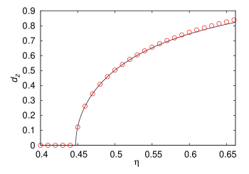
Figure 12: (Color online) Critical value of distance between channels as a function of the particle density in each channel. The solid line is the theoretical result and the open circles are the results from our MC simulations. We took the parameters $\upsilon=1$, $n=1$, and $\kappa=1$

Fig. 12 represents the critical separation between channels as a function of the particle density. This critical value corresponds to the separation $c_{z}$ where the zigzag transition takes place. This critical separation is calculated as the lower value of $c_{z}$ at which $\psi=0$ for a given $\eta$. For points below the curve in Fig. 12 the zigzag arrangement is the ground state configuration. The open red circles are the results for the zigzag transition points calculated from our MC simulations. The plotted region corresponds to the region where the zigzag transition is allowed, as was analyzed in previous section. One can see that there is perfect agreement between our theoretical results and the results from the MC simulations.

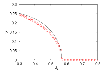
Figure 13: (Color online) Distance between channels as a function of the vertical separation between the channels, where the linear density in each channel is $\eta=0.52$. We took the parameters $\upsilon=1$, $n=1$, $\kappa=1$.

In Fig. 13 we show the distance between chains in the confinement direction as a function of the separation between the channels $c_{z}$ for a linear density $\eta=0.52$. The open circles show the results from our MC simulations and the solid line represents the value of the order parameter $\psi$ calculated from the present theory. The good agreement indicates that the Ginzburg-Landau theory is able to describe correctly the behavior of the system close to the zigzag transition point.

V Conclusions

We studied two coupled Q1D channels, consisting of a system of interacting charged particles confined by a parabolic trap in each channel, where the linear particle density in both channels is given by $\eta$. The ground state configuration at zero temperature was analyzed.

The structural transitions between phases were studied as a function of the linear density and the separation between the channels. We found a very rich phase diagram in case of vertically coupled channels, with first and second order transitions. The horizontally coupled system, on the other hand, exhibits a very restricted number of phases and all transitions are of first order. The latter can be traced back to the linear term in the relative distance between particles in the different channels, which appears in the energy expression. This linear term results in a rapid decrease of the interaction between channels.

Our simulations show that the zigzag transition occurs only in case of vertically coupled channels, which represent another effect of the linear term in the energy. In order to understand the behavior of this zigzag transition, we derived a Ginzburg-Landau equation and determined the behavior of the system close to the zigzag transition point. We analyzed the order parameter and its dependence on the linear density and the separation between channels. From theory we found that, for vertically coupled channels, an increase of the density produces a reduction of the first Brillouin zone of the Wigner crystal after the activation point $\eta_{act}$.  Within the density range where the zigzag transition is allowed, the vertical separation could be used as a tunable parameter to modulate the transition point. This result was found from theory and there is a perfect agreement with our numerical results, which shows that the presented theory is sufficient to understand the behavior and the nature of the zigzag transition in Q1D coupled channels.

VI Acknowledgments

This work was supported by the Flemish Science Foundation (FWO-Vl).

References

- (1) E. Wigner, Phys. Rev. 46, 1002 (1934)
- (2) R. W. Hasse and V. V. Avilov, Phys. Rev. A 44, 4506 (1991)
- (3) Y. G. Cornelissens, B. Partoens, and F. M. Peeters, Physica E 8, 314 (2000)
- (4) V. A. Schweigert and F. M. Peeters, Phys. Rev. B 51, 7700 (1995)
- (5) B. Partoens, V. A. Schweigert, and F. M. Peeters, Phys. Rev. Lett. 79, 3990 (1997)
- (6) W. M. Itano, J. J. Bollinger, J. N. Tan, B. Jelenkovic, X.-P. Huang, and D. J. Wineland, Science 279, 686 (1998)
- (7) I. Waki, S. Kassner, G. Birkl, and H. Walther, Phys. Rev. Lett. 68, 2007 (1992)
- (8) H. Ikegami, H. Akimoto, and K. Kono, Phys. Rev. Lett. 102, 046807 (2009)
- (9) A. Mortensen, E. Nielsen, T. Matthey, and M. Drewsen, Phys. Rev. Lett. 96, 103001 (2006)
- (10) D. H. E. Dubin and T. M. O’Neil, Rev. Mod. Phys. 71, 87 (1999)
- (11) G. Piacente, G. Q. Hai, and F. M. Peeters, Phys. Rev. B 81, 024108 (2010)
- (12) S. Fishman, G. De Chiara, T. Calarco, and G. Morigi, Phys. Rev. B 77, 064111 (2008)
- (13) K. Nelissen, B. Partoens, and C. Van den Broeck, Europhys. Lett. 88, 30001 (2009)
- (14) F. F. Munarin, K. Nelissen, W. P. Ferreira, G. A. Farias, and F. M. Peeters, Phys. Rev. E 77, 031608 (2008)
- (15) K. Nelissen, B. Partoens, and F. M. Peeters, Europhys. Lett. 79, 66001 (2007)
- (16) K. Nelissen, A. Matulis, B. Partoens, M. Kong, and F. M. Peeters, Phys. Rev. E 73, 016607 (2006)
- (17) G. Piacente, I. V. Schweigert, J. J. Betouras, and F. M. Peeters, Phys. Rev. B 69, 045324 (2004)
- (18) C. Lutz, M. Kollmann, and C. Bechinger, Phys. Rev. Lett. 93, 026001 (2004)
- (19) T. Y. M. Chan and S. John, Phys. Rev. A 78, 033812 (2008)
- (20) J. B. Delfau, C. Coste, and M. Saint Jean, Phys. Rev. E 84, 011101 (2011)
- (21) K. Nelissen, V. R. Misko, and F. M. Peeters, Europhys. Lett. 80, 56004 (2007)
- (22) J. C. N. Carvalho, K. Nelissen, W. P. Ferreira, G. A. Farias, and F. M. Peeters, Phys. Rev. E 85, 021136 (2012)
- (23) D. Lucena, D. V. Tkachenko, K. Nelissen, V. R. Misko, W. P. Ferreira, G. A. Farias, and F. M. Peeters, Phys. Rev. E 85, 031147 (2012)
- (24) W. Yang, K. Nelissen, M. Kong, Z. Zeng, and F. M. Peeters, Phys. Rev. E 79, 041406 (2009)
- (25) G. Karapetrov, M. V. Milosevic, M. Iavarone, J. Fedor, A. Belkin, V. Novosad, and F. M. Peeters, Phys. Rev. B 80, 180506 (2009)
- (26) D. Leibfried, B. DeMarco, V. Meyer, D. Lucas, M. Barret, J. Britton, W. M. Itano, B. Jelenkovic, C. Langer, T. Rosenband, and D. J. Wineland, Nature (London) 422, 412 (2003)
- (27) A. del Campo, G. De Chiara, G. Morigi, M. B. Plenio, and A. Retzker, New J. Phys. 12, 115003 (2010)
- (28) J. E. Galván-Moya and F. M. Peeters, Phys. Rev. B 84, 134106 (2011)
- (29) I. V. Schweigert, V. A. Schweigert, and F. M. Peeters, Phys. Rev. B 54, 10827 (1996)
- (30) D. I. Uzunov, Introduction to the Theory of Critical Phenomena (World Scientific Publishing, Singapore, 1993) pp. 63–66