Differentially Private Filtering

Abstract

Emerging systems such as smart grids or intelligent transportation systems often require end-user applications to continuously send information to external data aggregators performing monitoring or control tasks. This can result in an undesirable loss of privacy for the users in exchange of the benefits provided by the application. Motivated by this trend, this paper introduces privacy concerns in a system theoretic context, and addresses the problem of releasing filtered signals that respect the privacy of the user data streams. Our approach relies on a formal notion of privacy from the database literature, called differential privacy, which provides strong privacy guarantees against adversaries with arbitrary side information. Methods are developed to approximate a given filter by a differentially private version, so that the distortion introduced by the privacy mechanism is minimized. Two specific scenarios are considered. First, the notion of differential privacy is extended to dynamic systems with many participants contributing independent input signals. Kalman filtering is also discussed in this context, when a released output signal must preserve differential privacy for the measured signals or state trajectories of the individual participants. Second, differentially private mechanisms are described to approximate stable filters when participants contribute to a single event stream, extending previous work on differential privacy under continual observation.

I Introduction

A rapidly growing number of applications requires users to release private data streams to third-party applications for signal processing and decision-making purposes. Examples include smart grids, population health monitoring, online recommendation systems, traffic monitoring, fuel consumption optimization, and cloud computing for industrial control systems. For privacy or security reasons, the participants benefiting from the services provided by these systems generally do not want to release more information than strictly necessary. In a smart grid for example, a customer could receive better rates in exchange of continuously sending to the utility company her instantaneous power consumption, thereby helping to improve the demand forecast mechanism. In doing so however, she is also informing the utility or a potential eavesdropper about the type of appliances she owns as well as her daily activities [1]. Similarly, individual private signals can be recovered from published outputs aggregated from many users, and anonymizing a dataset is not enough to guarantee privacy, due to the existence of public side information. This is demonstrated in [2, 3] for example, where private ratings and transactions from individuals on commercial websites are successfully inferred with the help of information from public recommendation systems. Emerging traffic monitoring systems using position measurements from smartphones [4] is another application area where individual position traces can be re-identified by correlating them with public information such as a person’s location of residence or work [4]. Hence the development of rigorous privacy preserving mechanisms is crucial to address the justified concerns of potential users and thus encourage an increasing level of participation, which can in turn greatly improve the efficiency of these large-scale systems.

Precisely defining what constitutes a breach of privacy is a delicate task. A particularly successful recent definition of privacy used in the database literature is that of differential privacy [5], which is motivated by the fact that any useful information provided by a dataset about a group of people can compromise the privacy of specific individuals due to the existence of side information. Differentially private mechanisms randomize their responses to dataset analysis requests and guarantee that whether or not an individual chooses to contribute her data only marginally changes the distribution over the published outputs. As a result, even an adversary cross-correlating these outputs with other sources of information cannot infer much more about specific individuals after publication than before [6].

Most work related to privacy is concerned with the analysis of static databases [5, 7, 8, 9], whereas cyber-physical systems clearly emphasize the need for mechanisms working with dynamic, time-varying data streams. Recently, the problem of releasing differentially private statistics when the input data takes the form of a binary stream has been considered in [10, 11, 12]. This work is discussed in more details in Section VI-B. A differentially private version of the iterative averaging algorithm for consensus is considered in [13]. In this case, the input data to protect consists of the initial values of the participants and is thus a single vector, but the update mechanism subject to privacy attacks is dynamic. Information-theoretic approaches have also been proposed to guarantee some level of privacy when releasing time series [14, 15]. However, the resulting privacy guarantees only hold if the statistics of the participants’ data streams obey the assumptions made (typically stationarity, dependence and distributional assumptions), and require the explicit statistical modeling of all available side information. This task is very difficult in general as new, as-yet-unknown side information can become available after releasing the results. In contrast, differential privacy is a worst-case notion that holds independently of any probabilistic assumption on the dataset, and controls the information leakage against adversaries with arbitrary side information [6]. Once such a privacy guarantee is enforced, one can still leverage potential additional statistical information about the dataset to improve the quality of the outputs.

The main contribution of this paper is to introduce privacy concerns in the context of systems theory. Section II provides some technical background on differential privacy. We then formulate in Section III the problem of releasing the output of a dynamical system while preserving differential privacy for the driving inputs, assumed to originate from different participants. It is shown that accurate results can be published for systems with small incremental gains with respect to the individual input channels. These results are extended in Section IV to the problem of designing a differentially private Kalman filter, as an example of situation where additional information about the process generating the individual signals can be leveraged to publish more accurate results. Finally, Section VI is motivated by the recent work on “differential privacy under continual observation” [10, 11], and considers systems processing a single integer-valued signal describing the occurrence of events originating from many individual participants. Differentially private approximations of the systems are proposed with the goal of minimizing the mean squared error introduced by the privacy preserving mechanism. Some additional references to the related literature are provided in Section VI-B.

II Differential Privacy

In this section we review the notion of differential privacy [5] as well as some basic mechanisms that can be used to achieve it when the released data belongs to a finite-dimensional vector space. In the original papers on differential privacy [16, 5, 7], a sanitizing mechanism has access to a database and provides noisy answers to queries submitted by data analysts wishing to draw inference from the data. However, the notion of differential privacy can be defined for fairly general types of datasets. Most of the results in this section are known, but in some cases we provide more precise or slightly different versions of some statements made in previous work. We refer the reader to the surveys by Dwork, e.g., [17], for additional background on differential privacy.

II-A Definition

Let us fix some probability space $(\Omega,\mathcal{F},\mathbb{P})$. Let $\mathsf{D}$ be a space of datasets of interest (e.g., a space of data tables, or a signal space). A mechanism is just a map $M:\mathsf{D}\times\Omega\to\mathsf{R}$, for some measurable output space $(\mathsf{R},\mathcal{M})$, where $\mathcal{M}$ denotes a $\sigma$-algebra, such that for any element $d\in\mathsf{D}$, $M(d,\cdot)$ is a random variable, typically written simply $M(d)$. A mechanism can be viewed as a probabilistic algorithm to answer a query $q$, which is a map $q:\mathsf{D}\to\mathsf{R}$. In some cases, we index the mechanism by the query $q$ of interest, writing $M_{q}$.

Example 1.

Let $\mathsf{D}=\mathbb{R}^{n}$, with each real-valued entry of $d\in\mathsf{D}$ corresponding to some sensitive information for an individual contributing her data, e.g., her salary. A data analyst would like to know the average of the entries of $d$, i.e., the query is $q:\mathsf{D}\to\mathbb{R}$ with $q(d)=\frac{1}{n}\sum_{i=1}^{n}d_{i}$. As detailed in Section II-B, a typical mechanism $M_{q}$ to answer this query in a differentially private way computes $q(d)$ and blurs the result by adding a random variable $Y:\Omega\to\mathbb{R}$, so that $M_{q}:\mathsf{D}\times\Omega\to\mathbb{R}$ with $M_{q}(d)=\frac{1}{n}\sum_{i=1}^{n}d_{i}+Y$. Note that in the absence of perturbation $Y$, an adversary who knows $n$ and all $d_{j}$ for $j\geq 2$ can recover the remaining entry $d_{1}$ exactly if he learns $q(d)$. This can deter people from contributing their data, even though broader participation improves the accuracy of the analysis, which can provide useful knowledge to the population as a whole.

Next, we introduce the definition of differential privacy [5, 7]. Intuitively, in the following definition, $\mathsf{D}$ is a space of datasets of interest, and we have a symmetric binary relation Adj on $\mathsf{D}$, called adjacency, such that $\text{Adj}(d,d^{\prime})$ if and only if $d$ and $d^{\prime}$ differ by the data of a single participant.

Definition 1.

Let $\mathsf{D}$ be a space equipped with a symmetric binary relation denoted Adj, and let $(\mathsf{R},\mathcal{M})$ be a measurable space. Let $\epsilon,\delta\geq 0$. A mechanism $M:\mathsf{D}\times\Omega\to\mathsf{R}$ is $(\epsilon,\delta)$-differentially private if for all $d,d^{\prime}\in\mathsf{D}$ such that $\text{Adj}(d,d^{\prime})$, we have

$$\mathbb{P}(M(d)\in S)\leq e^{\epsilon}\mathbb{P}(M(d^{\prime})\in S)+\delta,\;\;\forall S\in\mathcal{M}.$$ (1)

If $\delta=0$, the mechanism is said to be $\epsilon$-differentially private.

Intuitively, this definition says that for two adjacent datasets, the distributions over the outputs of the mechanism should be close. The choice of the parameters $\epsilon,\delta$ is set by the privacy policy. Typically $\epsilon$ is taken to be a small constant, e.g., $\epsilon\approx 0.1$ or perhaps even $\ln 2$ or $\ln 3$. The parameter $\delta$ should be kept small as it controls the probability of certain significant losses of privacy, e.g., when a zero probability event for input $d^{\prime}$ becomes an event with positive probability for input $d$ in (1).

Remark 1.

The definition of differential privacy depends on the choice of $\sigma$-algebra $\mathcal{M}$ in Definition 1. When we need to state this $\sigma$-algebra explicitly, we write $M:\mathsf{D}\times\Omega\to(\mathsf{R},\mathcal{M})$. In particular, this $\sigma$-algebra should be sufficiently large, since (1) is trivially satisfied by any mechanism if $\mathcal{M}=\{\emptyset,\mathsf{R}\}$.

The next lemma provides alternative technical characterizations of differential privacy and appears to be new. First, we introduce some notation. We call a signed measure $\nu$ on $(\mathsf{R},\mathcal{M})$ $\delta$-bounded if it satisfies $\nu(S)\leq\delta$ for all $S\in\mathcal{M}$ [18, p.180]. A measure is sometimes called positive measure for emphasis. For $(\mathsf{R},\mathcal{M})$ a measurable space, we denote by $\mathcal{F}_{b}(\mathsf{R})$ the space of bounded real-valued measurable functions on $\mathsf{R}$ and we define $\mu g:=\int g\,d\mu$ for $g\in\mathcal{F}_{b}(\mathsf{R})$ and $\mu$ a positive measure on $\mathcal{M}$.

Lemma 1.

The following are equivalent:

1. $M$ is $(\epsilon,\delta)$-differentially private, satisfying (1).

2. For all $d,d^{\prime}\in\mathsf{D}$ such that $\text{Adj}(d,d^{\prime})$, there exists a $\delta$-bounded positive measure $\mu^{d,d^{\prime}}$ on $(\mathsf{R},\mathcal{M})$ such that we have

   $$\mathbb{P}(M(d)\in S)\leq e^{\epsilon}\mathbb{P}(M(d^{\prime})\in S)+\mu^{d,d^{\prime}}(S),\;\;\forall S\in\mathcal{M}.$$ (2)

3. For all $d,d^{\prime}\in\mathsf{D}$ such that $\text{Adj}(d,d^{\prime})$, there exists a $\delta$-bounded positive measure $\mu^{d,d^{\prime}}$ on $(\mathsf{R},\mathcal{M})$ such that for all $g\in\mathcal{F}_{b}(\mathsf{R})$, we have

   $$\mathbb{E}(g(M(d)))\leq e^{\epsilon}\mathbb{E}(g(M(d^{\prime})))+\mu^{d,d^{\prime}}g.$$ (3)

Proof.

(a) $\Rightarrow$ (b). Suppose that $M$ is $(\epsilon,\delta)$-differentially private. Define the signed measure $\nu^{d,d^{\prime}}$ by $S\mapsto\nu^{d,d^{\prime}}(S):=\mathbb{P}(M(d)\in S)-e^{\epsilon}\mathbb{P}(M(d^{\prime})\in S)$ [18, Section 5.6]. By the definition (1), $\nu^{d,d^{\prime}}$ is $\delta$-bounded. Let $\mu^{d,d^{\prime}}$ be the positive variation of $\nu^{d,d^{\prime}}$, i.e., $\mu^{d,d^{\prime}}(S)=\sup\{\nu(G):G\subset S\}$, for all $S\in\mathcal{M}$. Then $\mu^{d,d^{\prime}}$ is a positive measure [18, Section 5.6], is $\delta$-bounded since $\nu_{d,d^{\prime}}$ is, and since $\nu^{d,d^{\prime}}(S)\leq\mu^{d,d^{\prime}}(S)$ for all $S\in\mathcal{M}$, we have (2).

(b) $\Rightarrow$ (c): Let $B$ be a bound on $g$. For any $k\geq 1$, we divide the interval $[-B,B]$ in $k$ consecutive intervals $I_{i}$ of length $2B/k$, and we let $A_{i}=g^{-1}(I_{i})$ and $c_{i}$ be the mid-point of the interval $I_{i}$. Then (c) holds for the simple function $\sum_{i=1}^{k}c_{i}1_{A_{i}}$, and these functions approximate $g$. We conclude using the dominated convergence theorem.

(c) $\Rightarrow$ (a): Take $g=1_{S}$ and use the fact that $\mu^{d,d^{\prime}}$ is $\delta$-bounded. ∎

A fundamental property of the notion of differential privacy is that no additional privacy loss can occur by simply manipulating an output that is differentially private. This result is similar in spirit to the data processing inequality from information theory [19]. To state it, recall that a probability kernel between two measurable spaces $(\mathsf{R}_{1},\mathcal{M}_{1})$ and $(\mathsf{R}_{2},\mathcal{M}_{2})$ is a function $k:\mathsf{R}_{1}\times\mathcal{M}_{2}\to[0,1]$ such that $k(\cdot,S)$ is measurable for each $S\in\mathcal{M}_{2}$ and $k(r,\cdot)$ is a probability measure for each $r\in\mathsf{R}_{1}$.

Theorem 1 (Resilience to post-processing).

Let $M_{1}:\mathsf{D}\times\Omega\to(\mathsf{R}_{1},\mathcal{M}_{1})$ be an $(\epsilon,\delta)$-differentially private mechanism. Let $M_{2}:\mathsf{D}\times\Omega\to(\mathsf{R}_{2},\mathcal{M}_{2})$ be another mechanism, such that there exists a probability kernel $k:\mathsf{R}_{1}\times\mathcal{M}_{2}\to[0,1]$ verifying

$$\mathbb{P}(M_{2}(d)\in S|M_{1}(d))=k(M_{1}(d),S),\;\text{a.s.},\forall S\in\mathcal{M}_{2},\forall d\in\mathsf{D}.$$ (4)

Then $M_{2}$ is $(\epsilon,\delta)$-differentially private.

Note that in (4), the kernel $k$ is not allowed to depend on the dataset $d$. In other words, this condition says that once $M_{1}(d)$ is known, the distribution of $M_{2}(d)$ does not further depend on $d$. The theorem shows that a mechanism $M_{2}$ accessing a dataset only indirectly via the output of a differentially private mechanism $M_{1}$ cannot weaken the privacy guarantee. Hence post-processing can be used freely to improve the accuracy of an output, as in Section VI for example, without worrying about a possible loss of privacy.

Proof.

To the best of our knowledge, there is no previous proof of the resilience to post-processing theorem available for the case of randomized post-processing and $\delta>0$. Let $M_{1}$ be $(\epsilon,\delta)$-differentially private. We have, for two adjacent elements $d,d^{\prime}\in\mathsf{D}$ and for any $S\in\mathcal{M}_{2}$

$$\mathbb{P}(M_{2}(d)\in S) =\mathbb{E}[\mathbb{P}(M_{2}\in S|M_{1}(d))]=\mathbb{E}[k(M_{1}(d),S)]$$

$$\leq e^{\epsilon}\mathbb{E}[k(M_{1}(d^{\prime}),S)]+\int_{\mathsf{R}_{1}}k(m_{1},S)\;d\mu^{d,d^{\prime}}(m_{1})$$

$$=e^{\epsilon}\mathbb{P}(M_{2}(d^{\prime})\in S)+\nu^{d,d^{\prime}}(S).$$

The first equality is just the smoothing property of conditional expectations, and the inequality comes from (3) applied to the function $k(\cdot,S)$. Since $k$ is a probability kernel, the integral on the second line defines a measure $\nu^{d,d^{\prime}}$ on $\mathsf{R}_{2}$, which is $\delta$-bounded since $\nu^{d,d^{\prime}}(\mathsf{R}_{2})=\int_{\mathsf{R}_{1}}k(m_{1},\mathsf{R}_{2})d\mu^{d,d^{\prime}}(m_{1})=\int_{\mathsf{R}_{1}}1\;d\mu^{d,d^{\prime}}(m_{1})=\mu^{d,d^{\prime}}(\mathsf{R}_{1})\leq\delta$. ∎

II-B Basic Differentially Private Mechanisms

A mechanism that throws away all the information in a dataset is obviously private, but not useful, and in general one has to trade off privacy for utility when answering specific queries. We recall below two basic mechanisms that can be used to answer queries in a differentially private way. We are only concerned in this section with queries that return numerical answers, i.e., here a query is a map $q:\mathsf{D}\to\mathsf{R}$, where the output space $\mathsf{R}$ equals $\mathbb{R}^{k}$ for some $1\leq k<\infty$, is equipped with a norm denoted $\|\cdot\|_{\mathsf{R}}$, and the $\sigma$-algebra $\mathcal{M}$ on $\mathsf{R}$ is taken to be the standard Borel $\sigma$-algebra, denoted $\mathcal{R}^{k}$. The following quantity plays an important role in the design of differentially private mechanisms [5].

Definition 2.

Let $\mathsf{D}$ be a space equipped with an adjacency relation Adj. The sensitivity of a query $q:\mathsf{D}\to\mathsf{R}$ is defined as $\Delta_{\mathsf{R}}q:=\max_{d,d^{\prime}:\text{Adj}(d,d^{\prime})}\|q(d)-q(d^{\prime})\|_{\mathsf{R}}.$ In particular, for $\mathsf{R}=\mathbb{R}^{k}$ equipped with the $p$-norm $\|x\|_{p}=\left(\sum_{i=1}^{k}|x_{i}|^{p}\right)^{1/p}$ for $p\in[1,\infty]$, we denote the $\ell_{p}$ sensitivity by $\Delta_{p}q$.

II-B1 The Laplace Mechanism

This mechanism, proposed in [5], modifies an answer to a numerical query by adding i.i.d. zero-mean noise distributed according to a Laplace distribution. Recall that the Laplace distribution with mean zero and scale parameter $b$, denoted $\text{Lap}(b)$, has density $p(x;b)=\frac{1}{2b}\exp\left(-\frac{|x|}{b}\right)$ and variance $2b^{2}$. Moreover, for $w\in\mathbb{R}^{k}$ with $w_{i}$ iid and $w_{i}\sim\text{Lap}(b)$, denoted $w\sim\text{Lap}(b)^{k}$, we have $p(w;b)=(\frac{1}{2b})^{k}\exp\left(-\frac{\|w\|_{1}}{b}\right)$, $\mathbb{E}[\|w\|_{1}]=b$, and $\mathbb{P}(\|w\|_{1}\geq tb)=e^{-t}$.

Theorem 2.

Let $q:\mathsf{D}\to\mathbb{R}^{k}$ be a query. Then the Laplace mechanism $M_{q}:\mathsf{D}\times\Omega\to\mathbb{R}^{k}$ defined by $M_{q}(d)=q(d)+w$, with $w\sim\text{Lap}\left(b\right)^{k}$ and $b\geq\frac{\Delta_{1}q}{\epsilon}$ is $\epsilon$-differentially private.

Note that the mechanism requires each coordinate of $w$ to have standard deviation proportional to $\Delta_{1}q$, as well as inversely proportional to the privacy parameter $\epsilon$ (here $\delta=0)$. For example, if $q$ simply consists of $k$ repetitions of the same scalar query, then $\Delta_{1}q$ increases linearly with $k$, and the quadratically growing variance of the noise added to each coordinate prevents an adversary from averaging out the noise.

Proof.

We have, for $S\subset\mathbb{R}^{k}$ measurable and $d,d^{\prime}$ two adjacent datasets in $\mathsf{D}$,

$$P(M_{q}(d)\in S) =\left(\frac{1}{2b}\right)^{k}\int_{\mathbb{R}^{k}}1_{S}(q(d)+w)e^{-\frac{\|w\|_{1}}{b}}dw=\left(\frac{1}{2b}\right)^{k}\int_{\mathbb{R}^{k}}1_{S}(u)e^{-\frac{\|u-q(d)\|_{1}}{b}}dw$$

$$\leq e^{\frac{\|q(d)-q(d^{\prime})\|_{1}}{b}}\left(\frac{1}{2b}\right)^{k}\int_{\mathbb{R}^{k}}1_{S}(u)e^{-\frac{\|u-q(d^{\prime})\|_{1}}{b}}dw,$$

since $-\|u-q(d)\|_{1}\leq-\|u-q(d^{\prime})\|_{1}+\|q(d)-q(d^{\prime})\|_{1}$ by the triangle inequality. With the choice of $b=\Delta_{1}q/\epsilon$, we obtain the definition (1) of differential privacy (i.e., with $\delta=0$). ∎

II-B2 The Gaussian Mechanism

This mechanism, proposed in [7], is similar to the Laplace mechanism but adds i.i.d. Gaussian noise to obtain $(\epsilon,\delta)$-differential privacy, with $\delta>0$ but typically a smaller $\epsilon$ for the same utility. Recall the definition of the $\mathcal{Q}$-function

$$\mathcal{Q}(x):=\frac{1}{\sqrt{2\pi}}\int_{x}^{\infty}e^{-\frac{u^{2}}{2}}du.$$

The following theorem tightens the analysis from [7].

Theorem 3.

Let $q:\mathsf{D}\to\mathbb{R}^{k}$ be a query. Then the Gaussian mechanism $M_{q}:\mathsf{D}\times\Omega\to\mathbb{R}^{k}$ defined by $M_{q}(d)=q(d)+w$, with $w\sim\mathcal{N}\left(0,\sigma^{2}I_{k}\right)$, where $\sigma\geq\frac{\Delta_{2}q}{2\epsilon}(K+\sqrt{K^{2}+2\epsilon})$ and $K=\mathcal{Q}^{-1}(\delta)$, is $(\epsilon,\delta)$-differentially private.

Proof.

Let $d,d^{\prime}$ be two adjacent elements in $\mathsf{D}$, and denote $v:=q(d)-q(d^{\prime})$. We use the notation $\|\cdot\|$ for the $2$-norm in this proof. For $S\in\mathcal{R}^{k}$, we have

$$\mathbb{P}(M_{q}(d)\in S)=\frac{1}{(2\pi\sigma^{2})^{k/2}}\int_{\mathbb{R}^{k}}1_{S}(q(d)+w)e^{-\frac{\|w\|^{2}}{2\sigma^{2}}}dw=\frac{1}{(2\pi\sigma^{2})^{k/2}}\int_{\mathbb{R}^{k}}1_{S}(u)e^{-\frac{\|u-q(d)\|^{2}}{2\sigma^{2}}}du$$

$$=\frac{1}{(2\pi\sigma^{2})^{k/2}}\int_{S}e^{-\frac{\|u-q(d^{\prime})\|^{2}}{2\sigma^{2}}}e^{\frac{2(u-q(d^{\prime}))^{T}v-\|v\|^{2}}{2\sigma^{2}}}du$$

$$\leq e^{\epsilon}\mathbb{P}(M_{q}(d^{\prime})\in S)+\frac{1}{(2\pi\sigma^{2})^{k/2}}\int_{S}\bigg{[}e^{-\frac{\|u-q(d)\|^{2}}{2\sigma^{2}}}1\Big{\{}2(u-q(d^{\prime}))^{T}v\geq\|v\|^{2}+2\epsilon\sigma^{2}\Big{\}}\bigg{]}du.$$

The last integral term defines a measure $S\mapsto\mu^{d,d^{\prime}}(S)$ on $\mathbb{R}^{k}$ that we wish to bound by $\delta$. With the change of variables $y=(u-q(d))/\sigma$ and the choice $S=\mathbb{R}^{k}$ in the integral, we can rewrite it as $\mathbb{P}(Y^{T}v\geq\epsilon\sigma-\|v\|^{2}/2\sigma),$ with $Y\sim\mathcal{N}(0,I_{k})$. In particular, $Y^{T}v\sim\mathcal{N}(0,\|v\|^{2})$, hence is equal to $\|v\|Z$ in distribution, with $Z\sim\mathcal{N}(0,1)$. We are then led to set $\sigma$ sufficiently large so that $\mathbb{P}(Z\geq\epsilon\sigma/\|v\|-\|v\|/2\sigma)\leq\delta$, i.e., $\mathcal{Q}(\epsilon\sigma/\|v\|-\|v\|/2\sigma)\leq\delta$. The result then follows by straightforward calculation. ∎

As an illustration of the theorem, to guarantee $(\epsilon,\delta)$-differential privacy with $\epsilon=\ln 2$ and $\delta=0.05$, the standard deviation of the Gaussian noise should be about $2.65$ times the $\ell_{2}$ sensitivity of $q$. For the rest of the paper, we define $\kappa(\delta,\epsilon)=\frac{1}{2\epsilon}(K+\sqrt{K^{2}+2\epsilon}),$ so that the standard deviation $\sigma$ in Theorem 3 can be written $\sigma(\delta,\epsilon)=\kappa(\epsilon,\delta)\Delta_{2}q$. It can be shown that $\kappa(\delta,\epsilon)$ can be bounded by $O(\ln(1/\delta))^{1/2}/\epsilon$.

III Differentially Private Dynamic Systems

In this section we introduce the notion of differential privacy for dynamic systems. We start with some notations and technical prerequisites. All signals are discrete-time signals, start at time $0$, and all systems are assumed to be causal. For each time $T$, let $P_{T}$ be the truncation operator, so that for any signal $x$ we have

$$(P_{T}x)_{t}=\begin{cases}x_{t},&t\leq T\\ 0,&t>T.\end{cases}$$

Hence a deterministic system $\mathcal{G}$ is causal if and only if $P_{T}\mathcal{G}=P_{T}\mathcal{G}P_{T}$. We denote by $\ell_{p,e}^{m}$ the space of sequences with values in $\mathbb{R}^{m}$ and such that $x\in\ell_{p,e}^{m}$ if and only if $P_{T}x$ has finite $p$-norm for all integers $T$. The $\mathcal{H}_{2}$ norm and $\mathcal{H}_{\infty}$ norm of a stable transfer function $\mathcal{G}$ are defined respectively as $\|\mathcal{G}\|_{2}=\left(\frac{1}{2\pi}\int_{-\pi}^{\pi}\text{Tr}(\mathcal{G}^{*}(e^{i\omega})\mathcal{G}(e^{i\omega}))d\omega\right)^{1/2},\|\mathcal{G}\|_{\infty}=\text{ess}\sup_{\omega\in[-\pi,\pi)}\sigma_{\max}(\mathcal{G}(e^{i\omega})),$ where $\sigma_{\max}(A)$ denotes the maximum singular value of a matrix $A$.

We consider situations in which private participants contribute input signals driving a dynamic system and the queries consist of output signals of this system. First, in this section, we assume that the input of a system consists of $n$ signals, one for each participant. An input signal is denoted $u=(u_{1},\ldots,u_{n})$, with $u_{i}\in\ell_{r_{i},e}^{m_{i}}$ for some $m_{i}\in\mathbb{N}$ and $r_{i}\in[1,\infty]$. A simple example is that of a dynamic system releasing at each period the average over the past $l$ periods of the sum of the input values of the participants, i.e., with output $\frac{1}{l}\sum_{k=t-l+1}^{t}\sum_{i=1}^{n}u_{i,k}$ at time $t$, see Fig. 1. For $r=(r_{1},\ldots,r_{n})$ and $m=(m_{1},\ldots,m_{n})$, an adjacency relation can be defined on $l_{r,e}^{m}=\ell_{r_{1},e}^{m_{1}}\times\ldots\times\ell_{r_{n},e}^{m_{n}}$ for example by $\text{Adj}(u,u^{\prime})$ if and only if $u$ and $u^{\prime}$ differ by exactly one component signal, and moreover this deviation is bounded. That is, let us fix a set of nonnegative numbers $b=(b_{1},\ldots,b_{n})$, $b_{i}\geq 0$, and define

$$\text{Adj}^{b}(u,u^{\prime})\text{ iff for some }i,\|u_{i}-u_{i}^{\prime}\|_{r_{i}}\leq b_{i},\text{ and }u_{j}=u_{j}^{\prime}\text{ for all }j\neq i.$$ (5)

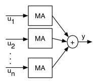
Figure 1: Illustrative example of a system computing the sum of the moving averages (MA) of input signals contributed by $n$ individual participants. A differentially private version of this system, for the adjacency relation (5), will guarantee to user $i$ that the distribution of the output signal does not vary significantly when her input varies in $r_{i}$-norm by at most $b_{i}$. In particular, the distribution of the output signal will not change significantly if user $i$’s input is zero ($u_{i}\equiv 0$, e.g., because the user is not present), or is not zero but satisfies $\|u_{i}\|_{r_{i}}\leq b_{i}$.

III-A Finite-Time Criterion for Differential Privacy

To approximate dynamic systems by versions respecting the differential privacy of the individual participants, we consider mechanisms of the form $M:\ell_{r,e}^{m}\times\Omega\to\ell_{s,e}^{m^{\prime}}$, i.e., producing for any input signal $u\in\ell_{r,e}^{m}$ a stochastic process $Mu$ with sample paths in $\ell_{s,e}^{m^{\prime}}$. As in the previous section, this requires that we first specify the measurable sets of $\ell_{s,e}^{m^{\prime}}$. We start by defining in a standard way the measurable sets of $(\mathbb{R}^{m^{\prime}})^{\mathbb{N}}$, the space of sequences with values in $\mathbb{R}^{m^{\prime}}$, to be the $\sigma$-algebra denoted $\mathcal{M}^{m^{\prime}}$ generated by the so-called finite-dimensional cylinder sets of the form $\{y\in(\mathbb{R}^{m^{\prime}})^{\mathbb{N}}:y_{0:T}\in H_{T}\},\text{for }T\geq 0$ and $H_{T}\in\mathcal{R}^{(T+1)m^{\prime}},$ where $y_{0:T}$ denotes the vector $[y_{0}^{T},\ldots,y_{T}^{T}]^{T}$ (see, e.g., [20, chapter 2]). The measurable sets considered for the output of $M$ are then obtained by intersection of $\ell_{s,e}^{m^{\prime}}$ with the sets of $\mathcal{M}^{m^{\prime}}$. The resulting $\sigma$-algebra is denoted $\mathcal{M}_{s,e}^{m^{\prime}}$ and is generated by the sets of the form

$$\tilde{H}_{T}=\{y\in\ell_{s,e}^{m^{\prime}}:y_{0:T}\in H_{T}\},\text{ for }T\geq 0,H_{T}\in\mathcal{R}^{(T+1)m^{\prime}}.$$ (6)

As for the dynamic systems of interest, we constrain in this paper the mechanisms to be causal, i.e., the distribution of $P_{T}Mu$ should be the same as that of $P_{T}MP_{T}u$ for any $u\in\ell_{r,e}^{m}$ and any time $T$. In other words, the values $u_{t}$ for $t>T$ do not influence the values of the mechanism output up to time $T$. The following technical lemma is useful to show that a mechanism on signal spaces is $(\epsilon,\delta)$-differentially private by considering only finite dimensional problems.

Lemma 2.

Consider an adjacency relation Adj on $\ell_{r,e}^{m}$. For a mechanism $M:\ell_{r,e}^{m}\times\Omega\to\ell_{s,e}^{m^{\prime}}$, the following are equivalent

1. $M$ is $(\epsilon,\delta)$-differentially private.

2. For all $u,u^{\prime}$ in $\ell_{r,e}^{m}$ such that $\text{Adj}(u,u^{\prime})$, we have

   $$\mathbb{P}((Mu)_{0:T}\in A)\leq e^{\epsilon}\,\mathbb{P}((Mu^{\prime})_{0:T}\in A)+\delta,\;\;\forall T\geq 0,\forall A\in\mathcal{R}^{(T+1)m^{\prime}}.$$ (7)

Proof.

$\ref{FTDP - enum 1})\Rightarrow\ref{FTDP - enum 2})$ If $M$ is $(\epsilon,\delta)$-differentially private, then for $u,u^{\prime}$ adjacent, and for all $H\in\mathcal{M}_{s,e}^{m^{\prime}}$, we have $\mathbb{P}(Mu\in H)\leq e^{\epsilon}\;\mathbb{P}(Mu^{\prime}\in H)+\delta$. In particular, for a given integer $T\geq 0$, we can restrict our attention to the sets $\tilde{H}_{T}$ of the form (6). In this case, we have immediately $\mathbb{P}(Mu\in\tilde{H}_{T})=\mathbb{P}((Mu)_{0:T}\in H_{T})$ since the events are the same.

$\ref{FTDP - enum 2})\Rightarrow\ref{FTDP - enum 1})$ Conversely, consider two adjacent signal $u,u^{\prime}\in\ell_{r,e}^{m}$, and let $S\in\mathcal{M}^{m^{\prime}}_{s,e}$, for which we want to show (1). Fix $\eta>0$. There exists $T\geq 0$ and $H_{T}\in\mathcal{R}^{(T+1)m^{\prime}}$ such that $\mathbb{P}(Mu\in S\Delta\tilde{H}_{T})\leq\eta$ and $\mathbb{P}(Mu^{\prime}\in S\Delta\tilde{H}_{T})\leq\eta$, where $A\Delta B:=(A\setminus B)\cup(B\setminus A)$ denotes the symmetric difference. This is a consequence for example of the fact that the finite-dimensional cylinder sets form an algebra and of the argument in the proof of [18, Theorem 3.1.10]. We then have

$$\mathbb{P}(Mu\in S) \leq\mathbb{P}(Mu\in\tilde{H}_{T})+\eta=\mathbb{P}((Mu)_{0:T}\in H_{T})+\eta$$

$$\leq e^{\epsilon}\,\mathbb{P}((Mu^{\prime})_{0:T}\in H_{T})+\delta+\eta=e^{\epsilon}\,\mathbb{P}(Mu^{\prime}\in\tilde{H}_{T})+\delta+\eta$$

$$\leq e^{\epsilon}\,\mathbb{P}(Mu^{\prime}\in S)+\delta+\eta(1+e^{\epsilon}).$$

Since $\eta$ can be taken arbitrarily small, the differential privacy definition (1) holds. ∎

III-B Basic Dynamic Mechanisms

Recall (see, e.g., [21]) that for a system $\mathcal{G}$ with inputs in $\ell_{r,e}^{m}$ and output in $\ell_{s,e}^{m^{\prime}}$, its $\ell_{r}$-to-$\ell_{s}$ incremental gain $\gamma^{inc}_{r,s}(\mathcal{G})$ is defined as the smallest number $\gamma$ such that

$$\|P_{T}\mathcal{G}u-P_{T}\mathcal{G}u^{\prime}\|_{s}\leq\gamma\|P_{T}u-P_{T}u^{\prime}\|_{r},\;\;\forall u,u^{\prime}\in\ell_{r,e}^{m},\;\forall T.$$

Now consider, for $r=(r_{1},\ldots,r_{n})$ and $m=(m_{1},\ldots,m_{n})$, a system $\mathcal{G}:l^{m}_{r,e}\to\ell_{s,e}^{m^{\prime}}$ defined by

$$\mathcal{G}(u_{1},\ldots,u_{n})=\sum_{i=1}^{n}\mathcal{G}_{i}u_{i},$$ (8)

where $\mathcal{G}_{i}:\ell_{r_{i},e}^{m_{i}}\to\ell_{s,e}^{m^{\prime}}$, for all $1\leq i\leq n$. The next theorem generalizes the Laplace and Gaussian mechanisms of Theorems 2 and 3 to causal dynamic systems.

Theorem 4.

Let $\mathcal{G}$ be defined as in (8) and consider the adjacency relation (5). Then the mechanism $Mu=\mathcal{G}u+w$, where $w$ is a white noise with $w_{t}\sim\text{Lap}(B/\epsilon)^{m^{\prime}}$ and $B\geq\max_{1\leq i\leq n}\{\gamma^{inc}_{r_{i},1}(\mathcal{G}_{i})\,b_{i}\}$, is $\epsilon$-differentially private. The mechanism is $(\epsilon,\delta)$-differentially private if $w_{t}\sim\mathcal{N}(0,\sigma^{2}I_{m^{\prime}})$, with $\sigma\geq\kappa(\delta,\epsilon)\max_{1\leq i\leq n}\{\gamma^{inc}_{r_{i},2}(\mathcal{G}_{i})\,b_{i}\}$.

Proof.

Consider two adjacent signals $u,u^{\prime}$, differing say in their $i^{\text{th}}$ component. Then, for $\alpha\in\{1,2\}$, we have

$$\|P_{T}\mathcal{G}u-P_{T}\mathcal{G}u^{\prime}\|_{\alpha} =\|P_{T}\mathcal{G}_{i}u_{i}-P_{T}\mathcal{G}_{i}u_{i}^{\prime}\|_{\alpha}\leq\gamma_{r_{i},\alpha}\|P_{T}u_{i}-P_{T}u_{i}^{\prime}\|_{r_{i}}$$

$$\leq\gamma_{r_{i},\alpha}\|u_{i}-u_{i}^{\prime}\|_{r_{i}}\leq\gamma_{r_{i},\alpha}b_{i}.$$

This leads to a bound on the $\ell_{1}$ and $\ell_{2}$ sensitivity of $P_{T}\mathcal{G}$, valid for all $T$. The result is then an application of Theorems 2 and 3 and Lemma 2, since (7) is satisfied for all $T$. ∎

Corollary 1.

Let $\mathcal{G}$ be defined as in (8) with each system $\mathcal{G}_{i}$ linear, and $r_{i}=2$ for all $1\leq i\leq n$. Then the mechanism $Mu=\mathcal{G}u+w$, where $w$ is a white Gaussian noise with $w_{t}\sim\mathcal{N}(0,\sigma^{2}I_{m^{\prime}})$ and $\sigma\geq\kappa(\delta,\epsilon)\max_{1\leq i\leq n}\{\|\mathcal{G}_{i}\|_{\infty}\,b_{i}\}$, is $(\epsilon,\delta)$-differentially private for (5).

III-C Filter Approximation Set-ups for Differential Privacy

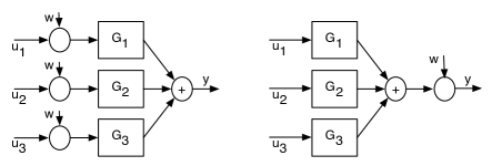
Figure 2: Two architectures for differential privacy. (a) Input perturbation. (b) Output perturbation.

Let $r_{i}=2$ for all $i$ and $\mathcal{G}$ be linear as in the Corollary 1, and assume for simplicity the same bound $b_{1}^{2}=\ldots=b_{n}^{2}=B$ for the allowed variations in energy of each input signal. We have then two simple mechanisms producing a differentially private version of $\mathcal{G}$, depicted on Fig. 2. The first one directly perturbs each input signal $u_{i}$ by adding to it a white Gaussian noise $w_{i}$ with $w_{i,t}\sim\mathcal{N}(0,\sigma^{2}I_{m_{i}})$ and $\sigma^{2}=\kappa(\delta,\epsilon)^{2}B$. These perturbations on each input channel are then passed through $\mathcal{G}$, leading to a mean squared error (MSE) for the output equal to $\kappa(\delta,\epsilon)^{2}B\|\mathcal{G}\|^{2}_{2}=\kappa(\delta,\epsilon)^{2}B\sum_{i=1}^{n}\|\mathcal{G}_{i}\|^{2}_{2}$. Alternatively, we can add a single source of noise at the output of $\mathcal{G}$ according to Corollary 1, in which case the MSE is $\kappa(\delta,\epsilon)^{2}B\max_{1\leq i\leq n}\{\|\mathcal{G}_{i}\|_{\infty}^{2}\}$. Both of these schemes should be evaluated depending on the system $\mathcal{G}$ and the number $n$ of participants, as none of the error bound is better than the other in all circumstances. For example, if $n$ is small or if the bandwidths of the individual transfer functions $\mathcal{G}_{i}$ do not overlap, the error bound for the input perturbation scheme can be smaller. Another advantage of this scheme is that the users can release differentially private signals themselves without relying on a trusted server. However, there are cryptographic means for achieving the output perturbation scheme without centralized trusted server as well, see, e.g., [22].

Example 2.

Consider again the problem of releasing the average over the past $l$ periods of the sum of the input signals, i.e., $\mathcal{G}=\sum_{i=1}^{n}\mathcal{G}_{i}$ with $(\mathcal{G}_{i}u_{i})_{t}=\frac{1}{l}\sum_{k=t-l+1}^{t}u_{i,k}$, for all $i$. Then $\|\mathcal{G}_{i}\|_{2}^{2}=1/l$, whereas $\|\mathcal{G}_{i}\|_{\infty}=1$, for all $i$. The MSE for the scheme with the noise at the input is then $\kappa(\delta,\epsilon)^{2}Bn/l$. With the noise at the output, the MSE is $\kappa(\delta,\epsilon)^{2}B$, which is better exactly when $n>l$, i.e., the number of users is larger than the averaging window.

IV Differentially Private Kalman Filtering

We now discuss the Kalman filtering problem subject to a differential privacy constraint. Compared to the previous section, for Kalman filtering it is assumed that more is publicly known about the dynamics of the processes producing the individual signals. The goal here is to guarantee differential privacy for the individual state trajectories. Section V describes an application of the privacy mechanisms presented here to a traffic monitoring problem.

IV-A A Differentially Private Kalman Filter

Consider a set of $n$ linear systems, each with independent dynamics

$$x_{i,t+1}=A_{i}x_{i,t}+B_{i}w_{i,t},\;\;t\geq 0,\;\;1\leq i\leq n,$$ (9)

where $w_{i}$ is a standard zero-mean Gaussian white noise process with covariance $\mathbb{E}[w_{i,t}w_{i,t^{\prime}}]=\delta_{t-t^{\prime}}$, and the initial condition $x_{i,0}$ is a Gaussian random variable with mean $\bar{x}_{i,0}$, independent of the noise process $w_{i}$. System $i$, for $1\leq i\leq n$, sends measurements

$$y_{i,t}=C_{i}x_{i,t}+D_{i}w_{i,t}$$ (10)

to a data aggregator. We assume for simplicity that the matrices $D_{i}$ are full row rank. Figure 3 shows this initial set-up.

The data aggregator aims at releasing a signal that asymptotically minimizes the minimum mean squared error with respect to a linear combination of the individual states. That is, the quantity of interest to be estimated at each period is $z_{t}=\sum_{i=1}^{n}L_{i}x_{i,t}$, where $L_{i}$ are given matrices, and we are looking for a causal estimator $\hat{z}$ constructed from the signals $y_{i},1\leq i\leq n$, solution of

$$\min_{\hat{z}}\lim_{T\to\infty}\frac{1}{T}\sum_{t=0}^{T-1}\mathbb{E}\left[\|z_{t}-\hat{z}_{t}\|_{2}^{2}\right].$$

The data $\bar{x}_{i,0},A_{i},B_{i},C_{i},D_{i},L_{i},1\leq i\leq n,$ are assumed to be public information. For all $1\leq i\leq n$, we assume that the pairs $(A_{i},C_{i})$ are detectable and the pairs $(A_{i},B_{i})$ are stabilizable. In the absence of privacy constraint, the optimal estimator is $\hat{z}_{t}=\sum_{i=1}^{n}L_{i}\hat{x}_{i,t}$, with $\hat{x}_{i,t}$ provided by the steady-state Kalman filter estimating the state of system $i$ from $y_{i}$ [23], and denoted $\mathcal{K}_{i}$ in the following.

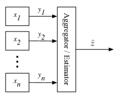
Figure 3: Kalman filtering set-up.

Suppose now that the publicly released estimate should guarantee the differential privacy of the participants. This requires that we first specify an adjacency relation on the appropriate space of datasets. Let $x=[x_{1}^{T},\ldots,x_{n}^{T}]^{T}$ and $y=[y_{1}^{T},\ldots,y_{n}^{T}]^{T}$ denote the global state and measurement signals. Assume that the mechanism is required to guarantee differential privacy with respect to a subset $\mathcal{S}_{i}:=\{i_{1},\ldots,i_{k}\}$ of the coordinates of the state trajectory $x_{i}$. Let the selection matrix $S_{i}$ be the diagonal matrix with $[S_{i}]_{jj}=1$ if $j\in\mathcal{S}_{i}$, and $[S_{i}]_{jj}=0$ otherwise. Hence $S_{i}v$ sets the coordinates of a vector $v$ which do not belong to the set $\mathcal{S}_{i}$ to zero. Fix a vector $\rho\in\mathbb{R}_{+}^{n}$. The adjacency relation considered here is

$$\text{Adj}_{\mathcal{S}}^{\rho}(x,x^{\prime})\text{ iff }\text{for some }i, \;\|S_{i}x_{i}-S_{i}x_{i}^{\prime}\|_{2}\leq\rho_{i},(I-S_{i})x_{i}=(I-S_{i})x_{i}^{\prime},$$ (11)

$$\text{and }x_{j}=x_{j}^{\prime}\text{ for all }j\neq i.$$

In words, two adjacent global state trajectories differ by the values of a single participant, say $i$. Moreover, for differential privacy guarantees we are constraining the range in energy variation in the signal $S_{i}x_{i}$ of participant $i$ to be at most $\rho_{i}^{2}$. Hence, the distribution on the released results should be essentially the same if a participant’s state signal value $S_{i}x_{i,t_{0}}$ at some single specific time $t_{0}$ were replaced by $S_{i}x^{\prime}_{i,t_{0}}$ with $\|S_{i}(x_{i,t_{0}}-x^{\prime}_{i,t_{0}})\|\leq\rho_{i}$, but the privacy guarantee should also hold for smaller instantaneous deviations on longer segments of trajectory. Other adjacency relations could be considered, e.g., directly on the measured signals $y$ or more generally on linear combinations of the components of individual states.

Depending on which signals on Fig. 3 are actually published, and similarly to the discussion of Section III-C, there are different points at which a privacy inducing noise can be introduced. First, for the input noise injection mechanism, the noise can be added by each participant directly to their transmitted measurement signal $y_{i}$. Namely, since for two state trajectories $x_{i},x_{i}^{\prime}$ adjacent according to (11) we have $x_{i}-x_{i}^{\prime}=S_{i}(x_{i}-x_{i}^{\prime})$, the variation for the corresponding measured signals can be bounded as follows

$$\|y_{i}-y_{i}^{\prime}\|_{2}=\|C_{i}S_{i}(x_{i}-x_{i}^{\prime})\|_{2}=\|C_{i}S_{i}S_{i}(x_{i}-x_{i}^{\prime})\|_{2}\leq\sigma_{\max}(C_{i}S_{i})\rho_{i}.$$

Hence differential privacy can be guaranteed if participant $i$ adds to $y_{i}$ a white Gaussian noise with covariance matrix $\kappa(\delta,\epsilon)^{2}\rho_{i}^{2}\sigma^{2}_{\max}(C_{i}S_{i})I_{p_{i}}$, where $p_{i}$ is the dimension of $y_{i,t}$. Note that in this sensitivity computation the measurement noise $D_{i}w_{i}$ has the same realization independently of the considered variation in $x_{i}$. At the data aggregator, the privacy-preserving noise can be taken into account in the design of the Kalman filter, since it can be viewed as an additional measurement noise. Again, an advantage of this mechanism is its simplicity of implementation when the participants do not trust the data aggregator, since the transmitted signals are already differentially private.

Next, consider the output noise injection mechanism. Since we assume that $\bar{x}^{i}_{0}$ is public information, the initial condition $\hat{x}_{i,0}$ of each state estimator is fixed. Consider now two state trajectories $x,x^{\prime}$, adjacent according to (11), and let $\hat{z},\hat{z}^{\prime}$ be the corresponding estimates produced by the Kalman filters. We have

$$\hat{z}-\hat{z}^{\prime}=L_{i}\mathcal{K}_{i}(y_{i}-y_{i}^{\prime})=L_{i}\mathcal{K}_{i}C_{i}S_{i}(x_{i}-x_{i}^{\prime}),$$

where we recall that $\mathcal{K}_{i}$ is the $i^{th}$ Kalman filter. Hence $\|\hat{z}-\hat{z}^{\prime}\|_{2}\leq\gamma_{i}\rho_{i},$ where $\gamma_{i}$ is the $\mathcal{H}_{\infty}$ norm of the transfer function $L_{i}\mathcal{K}_{i}C_{i}S_{i}$. We thus have the following theorem.

Theorem 5.

A mechanism releasing $\left(\sum_{i=1}^{n}L_{i}\mathcal{K}_{i}y_{i}\right)+\gamma\;\kappa(\delta,\epsilon)\;\nu$, where $\nu$ is a standard white Gaussian noise independent of $\{w_{i}\}_{1\leq i\leq n},\{x_{i,0}\}_{1\leq i\leq n}$, and $\gamma=\max_{1\leq i\leq n}\{\gamma_{i}\rho_{i}\}$, with $\gamma_{i}$ the $\mathcal{H}_{\infty}$ norm of $L_{i}\mathcal{K}_{i}C_{i}S_{i}$, is differentially private for the adjacency relation (11).

IV-B Filter Redesign for Stable Systems

In the case of the output perturbation mechanism, one can potentially improve the MSE performance of the filter with respect to the Kalman filter used in the previous subsection. Namely, consider the design of $n$ filters of the form

$$\hat{x}_{i,t+1} =F_{i}\hat{x}_{i,t}+G_{i}y_{i,t}$$ (12)

$$\hat{z}_{i,t} =H_{i}\hat{x}_{i,t}+K_{i}y_{i,t},$$ (13)

for $1\leq i\leq n$, where $F_{i},G_{i},H_{i},K_{i}$ are matrices to determine. The estimator considered is $\hat{z}_{t}=\sum_{i=1}^{n}\hat{z}_{i,t}$, so that each filter output $\hat{z}_{i}$ should minimize the steady-state MSE with $z_{i}=L_{i}x_{i}$, and the released signal should guarantee differential privacy with respect to (11). Assume first in this section that the system matrices $A_{i}$ are stable, in which case we also restrict the filter matrices $F_{i}$ to be stable. Moreover, we only consider the design of full order filters, i.e., the dimensions of $F_{i}$ are greater or equal to those of $A_{i}$, for all $1\leq i\leq n$.

Denote the overall state for each system and associated filter by $\tilde{x}_{i}=[x_{i}^{T},\hat{x}_{i}^{T}]^{T}$. The combined dynamics from $w_{i}$ to the estimation error $e_{i}:=z_{i}-\hat{z}_{i}$ can be written

$$\tilde{x}_{i,t+1} =\tilde{A}_{i}\tilde{x}_{i,t}+\tilde{B}_{i}w_{i,t}$$

$$e_{i,t} =\tilde{C}_{i}\tilde{x}_{i,t}+\tilde{D}_{i}w_{i,t},$$

where

$$\tilde{A}_{i}=\begin{bmatrix}A_{i}&0\\ G_{i}C_{i}&F_{i}\end{bmatrix},\;\;\tilde{B}_{i}=\begin{bmatrix}B_{i}\\ G_{i}D_{i}\end{bmatrix},\;\;\tilde{C}_{i}=\begin{bmatrix}L_{i}-K_{i}C_{i}&-H_{i}\end{bmatrix},\;\;\tilde{D}_{i}=-K_{i}D_{i}.$$

The steady-state MSE for the $i^{th}$ estimator is then $\lim_{t\to\infty}\mathbb{E}[e_{i,t}^{T}e_{i,t}]$. Moreover, we are interested in designing filters with small $\mathcal{H}_{\infty}$ norm, in order to minimize the amount of noise introduced by the privacy-preserving mechanism, which ultimately also impacts the overall MSE. Considering as in the previous subsection the sensitivity of filter $i$’s output to a change from a state trajectory $x$ to an adjacent one $x^{\prime}$ according to (11), and letting $\delta x_{i}=x_{i}-x_{i}^{\prime}=S_{i}(x_{i}-x_{i}^{\prime})=S_{i}\delta x_{i}$, we see that the change in the output of filter $i$ follows the dynamics

$$\delta\hat{x}_{i,t+1} =F_{i}\delta\hat{x}_{i,t}+G_{i}C_{i}S_{i}\delta x_{i}$$

$$\delta\hat{z}_{i} =H_{i}\delta\hat{x}_{i,t}+K_{i}C_{i}S_{i}\delta x_{i}.$$

Hence the $\ell_{2}$-sensitivity can be measured by the $\mathcal{H}_{\infty}$ norm of the transfer function

$$\left[\begin{array}[]{c|c}{F_{i}}&{G_{i}C_{i}S_{i}}\\ \hline\cr{H_{i}}&{K_{i}C_{i}S_{i}}\end{array}\right].$$ (16)

Simply replacing the Kalman filter in Theorem 5, the MSE for the output perturbation mechanism guaranteeing $(\epsilon,\delta)$-privacy is then

$$\sum_{i=1}^{n}\|\tilde{C}_{i}(zI-\tilde{A}_{i})^{-1}\tilde{B}_{i}+\tilde{D}_{i}\|_{2}^{2}+\kappa(\delta,\epsilon)^{2}\max_{1\leq i\leq n}\{\gamma_{i}^{2}\rho_{i}^{2}\},$$

$$\text{with }\gamma_{i}:=\|H_{i}(zI-F_{i})^{-1}G_{i}C_{i}S_{i}+K_{i}C_{i}S_{i}\|_{\infty}.$$

Hence minimizing this MSE leads us to the following optimization problem

$$\min_{\mu_{i},\lambda,F_{i},G_{i},H_{i},K_{i}}\quad\sum_{i=1}^{n}\mu_{i}+\kappa(\delta,\epsilon)^{2}\lambda$$ (17)

$$\text{s.t. }\forall\;1\leq i\leq n,\|\tilde{C}_{i}(zI-\tilde{A}_{i})^{-1}\tilde{B}_{i}+\tilde{D}_{i}\|_{2}^{2}\leq\mu_{i},$$ (18)

$$\rho_{i}^{2}\|H_{i}(zI-F_{i})^{-1}G_{i}C_{i}S_{i}+K_{i}C_{i}S_{i}\|^{2}_{\infty}\leq\lambda.$$ (19)

Assume without loss of generality that $\rho_{i}>0$ for all $i$, since the privacy constraint for the signal $x_{i}$ vanishes if $\rho_{i}=0$. The following theorem gives a convex sufficient condition in the form of Linear Matrix Inequalities (LMIs) guaranteeing that a choice of filter matrices $F_{i},G_{i},H_{i},K_{i}$ satisfies the constraints (18)-(19).

Theorem 6.

The constraints (18)-(19), for some $1\leq i\leq n$, are satisfied if there exists matrices $W_{i},Y_{i},Z_{i},\hat{F}_{i},\hat{G}_{i},\hat{H}_{i},\hat{K}_{i}$ such that $\text{Tr}(W_{i})<\mu_{i}$,

$$\begin{bmatrix}W_{i}&(L_{i}-\hat{K}_{i}C_{i}-\hat{H}_{i})&(L_{i}-\hat{K}_{i}C_{i})&-\hat{K}_{i}D_{i}\\ *&Z_{i}&Z_{i}&0\\ *&*&Y_{i}&0\\ *&*&*&I\end{bmatrix}\succ 0,$$

$$\begin{bmatrix}Z_{i}&Z_{i}&Z_{i}A_{i}&Z_{i}A_{i}&Z_{i}B_{i}\\ *&Y_{i}&(Y_{i}A_{i}+\hat{G}_{i}C_{i}+\hat{F}_{i})&(Y_{i}A_{i}+\hat{G}_{i}C_{i})&(Y_{i}B_{i}+\hat{G}_{i}D_{i})\\ *&*&Z_{i}&Z_{i}&0\\ *&*&*&Y_{i}&0\\ *&*&*&*&I\end{bmatrix}\succ 0,$$

$$\text{and }\;\;\begin{bmatrix}Z_{i}&Z_{i}&0&0&0&0\\ *&Y_{i}&0&\hat{F}_{i}&0&\hat{G}_{i}C_{i}S_{i}\\ *&*&\frac{\lambda}{\rho^{2}_{i}}I&\hat{H}_{i}&0&\hat{K}_{i}C_{i}S_{i}\\ *&*&*&Z_{i}&Z_{i}&0\\ *&*&*&*&Y_{i}&0\\ *&*&*&*&*&I\end{bmatrix}\succ 0.$$

If these conditions are satisfied, one can recover admissible filter matrices $F_{i},G_{i},H_{i},K_{i}$ by setting

$$F_{i}=V_{i}^{-1}\hat{F}_{i}\hat{Z}_{i}^{-1}U_{i}^{-T},\;\;G_{i}=V_{i}^{-1}\hat{G}_{i},\;\;H_{i}=\hat{H}_{i}Z_{i}^{-1}U_{i}^{-T},\;\;K_{i}=\hat{K}_{i}$$ (20)

where $U_{i},V_{i}$ are any two nonsingular matrices such that $V_{i}U_{i}^{T}=I-Y_{i}Z_{i}^{-1}$.

Proof.

For simplicity of notation, let us remove the subscript $i$ in the constraints (18)-(19), since we are considering the design of the filters individually. Also, define $\bar{\lambda}=\lambda/\rho^{2}$. The condition (18) is satisfied if and only if there exist matrices $W,\tilde{P}_{1}$ such that [24]

$$\text{Tr}(W)<\mu,\quad\begin{bmatrix}W&\tilde{C}&\tilde{D}\\ *&\tilde{P}_{1}&0\\ *&*&I\end{bmatrix}\succ 0,\quad\begin{bmatrix}\tilde{P}_{1}&\tilde{P}_{1}\tilde{A}&\tilde{P}_{1}\tilde{B}\\ *&\tilde{P}_{1}&0\\ *&*&I\end{bmatrix}\succ 0.$$ (21)

For the constraint (19), first note that we have equality of the transfer functions

$$\left[\begin{array}[]{c|c}{F}&{GCS}\\ \hline\cr{H}&{KCS}\end{array}\right]=\left[\begin{array}[]{c|c}{\begin{array}[]{cc}A_{1}&0\\ 0&F\end{array}}&{\begin{array}[]{c}0\\ GCS\end{array}}\\ \hline\cr{\begin{array}[]{cc}0&H\end{array}}&{KCS}\end{array}\right]$$

for any matrix $A_{1}$, in particular for $A_{1}$ the zero matrix of the same dimensions as $A$. With this choice, denote

$$\bar{A}=\begin{bmatrix}0&0\\ 0&F\end{bmatrix},\;\;\bar{B}=\begin{bmatrix}0\\ GCS\end{bmatrix},\bar{C}=\begin{bmatrix}0&H\end{bmatrix},\bar{D}=KCS.$$

Then the constraint (19) can be rewritten $\|\bar{C}(sI-\bar{A})^{-1}\bar{B}+\bar{D}\|_{\infty}<\bar{\lambda},$ and is satisfied if and only if there exists a matrix $\tilde{P}_{2}$, of the same dimensions as $\tilde{P}_{1}$, such that [24]

$$\begin{bmatrix}\tilde{P}_{2}&0&\tilde{P}_{2}\bar{A}&\tilde{P}_{2}\bar{B}\\ *&\bar{\lambda}I&\bar{C}&\bar{D}\\ *&*&\tilde{P}_{2}&0\\ *&*&*&I\end{bmatrix}\succ 0.$$ (22)

The sufficient condition of the theorem is obtained by adding the constraint

$$\tilde{P}:=\tilde{P}_{1}=\tilde{P}_{2}$$ (23)

and using the change of variable suggested in [25, p. 902]. Namely, assume that there are matrices $F,G,H,K,\tilde{P}$, and $W$ satisfying (21), (22), (23). We partition the positive definite matrix $\tilde{P}$ and its inverse as

$$\tilde{P}=\begin{bmatrix}Y&V\\ V^{T}&\hat{Y}\end{bmatrix},\quad\tilde{P}^{-1}=\begin{bmatrix}X&U\\ U^{T}&\hat{X}\end{bmatrix}.$$

Note that $YX+VU^{T}=I$. Define

$$J_{1}=\begin{bmatrix}X&I\\ U^{T}&0\end{bmatrix},\quad J_{2}=\begin{bmatrix}I&Y\\ 0&V^{T}\end{bmatrix}.$$ (24)

Then we have $\tilde{P}J_{1}=J_{2}$. Moreover

$$J_{1}^{T}\tilde{P}J_{1}=\begin{bmatrix}X&I\\ I&Y\end{bmatrix},\quad J_{1}^{T}\tilde{P}\tilde{A}J_{1}=\begin{bmatrix}AX&A\\ YAX+VGCX+VFU^{T}&YA+VGC\end{bmatrix},$$

$$J_{1}^{T}\tilde{P}\tilde{B}=\begin{bmatrix}B\\ YB+VGD\end{bmatrix},\quad\tilde{C}J_{1}=\begin{bmatrix}(L-KC)X-HU^{T}&L-KC\end{bmatrix}.$$

Similarly,

$$J_{1}^{T}\tilde{P}\bar{A}J_{1}=\begin{bmatrix}0&0\\ VFU^{T}&0\end{bmatrix},\quad J_{1}^{T}\tilde{P}\bar{B}=\begin{bmatrix}0\\ VGCS\end{bmatrix},\quad\bar{C}J_{1}=\begin{bmatrix}HU^{T}&0\end{bmatrix}.$$

Let $Z=X^{-1}$. Consider first the congruence transformations

• of the first LMI in (21) by $\text{diag}(I,J_{1},I)$ and then by $\text{diag}(I,Z,I,I)$,

• of the second LMI in (21) by $\text{diag}(J_{1},J_{1},I)$, and then by $\text{diag}(Z,I,Z,I,I)$,

• and of the LMI (22) by $\text{diag}(J_{1},I,J_{1},I)$, and then by $\text{diag}(Z,I,I,Z,I,I)$.

Then, the transformation $\hat{F}=VFU^{T}Z,\hat{G}=VG,\hat{H}=HU^{T}Z,$ between the filter matrix variables $F,G,H$ and the new variables $\hat{F},\hat{G},\hat{H}$ leads to the LMIs of the theorem. Hence these LMIs are necessarily satisfied if the constraints (21), (22) are satisfied together with (23).

Now suppose that the LMIs of the theorem are satisfied. Since $Z\succ 0$, we can define $X=Z^{-1}$. Moreover, since $\begin{bmatrix}Z&Z\\ Z&Y\end{bmatrix}\succ 0$, we have $Y\succ X^{-1}$ by taking the Schur complement, and so $I-XY$ is nonsingular. Hence we can find two $n\times n$ nonsingular matrices $U,V$ such that $UV^{T}=I-XY$. Then define the nonsingular matrices $J_{1},J_{2}$ as in (24), let $\tilde{P}=J_{2}J_{1}^{-1}$, and define the matrices $F,G,H,K$ as in (20). Since $J_{1}$ is nonsingular, we can then reverse the congruence transformations to recover (21), (22), which shows that the constraints (18), (19) are satisfied. ∎

Note that the problem (17) is also linear in $\mu_{i},\lambda$. These variables can then be minimized subject to the LMI constraints of Theorem 6 in order to design a good filter trading off estimation error and $\ell^{2}$-sensitivity to minimize the overall MSE. However, including these variables directly in the optimization problem can lead to ill-conditioning in the inversion of the matrices $U_{i},V_{i}$ in (20), a phenomenon discussed together with a recommended fix in [25, p. 903].

IV-C Unstable Systems

If the dynamics (9) are not stable, the linear filter design approach presented in the previous paragraph is not valid. To handle this case, we can further restrict the class of filters. As before we minimize the estimation error variance together with the sensitivity measured by the $\mathcal{H}_{\infty}$ norm of the filter. Starting from the general linear filter dynamics (12), (13), we can consider designs where $\hat{x}_{i}$ is an estimate of $x_{i}$, and set $H_{i}=L_{i},K_{i}=0,$ so that $\hat{z}_{i}=L_{i}\hat{x}_{i}$ is an estimate of $z_{i}=L_{i}x_{i}$. The error dynamics $e_{i}:=x_{i}-\hat{x}_{i}$ then satisfies

$$e_{i,t+1}=(A_{i}-G_{i}C_{i})x_{i,t}-F_{i}\hat{x}_{i,t}+(B_{i}-G_{i}D_{i})w_{i,t}.$$

Setting $F_{i}=(A_{i}-G_{i}C_{i})$ gives an error dynamics independent of $x_{i}$

$$e_{i,t+1}=(A_{i}-G_{i}C_{i})e_{i,t}+(B_{i}-G_{i}D_{i})w_{i,t},$$ (25)

and leaves the matrix $G_{i}$ as the only remaining design variable. Note however that the resulting class of filters contains the (one-step delayed) Kalman filter. To obtain a bounded error, there is an implicit constraint on $G_{i}$ that $A_{i}-G_{i}C_{i}$ should be stable.

Now, following the discussion in the previous subsection, minimizing the MSE while enforcing differential privacy leads to the following optimization problem

$$\min_{\mu_{i},\lambda,G_{i}}\quad\sum_{i=1}^{n}\mu_{i}+\kappa(\delta,\epsilon)^{2}\lambda$$ (26)

$$\text{s.t. }\;\forall\;1\leq i\leq n,\;\;\|L_{i}(zI-(A_{i}-G_{i}C_{i}))^{-1}(B_{i}-G_{i}D_{i})\|_{2}^{2}\leq\mu_{i},$$ (27)

$$\rho_{i}^{2}\|L_{i}(zI-(A_{i}-G_{i}C_{i}))^{-1}G_{i}C_{i}S_{i}\|^{2}_{\infty}\leq\lambda.$$ (28)

Again, one can efficiently check a sufficient condition, in the form of the LMIs of the following theorem, guaranteeing that the constraints (27), (28) are satisfied. Optimizing over the variables $\lambda_{i},\mu_{i},G_{i}$ can then be done using semidefinite programming.

Theorem 7.

The constraints (27)-(28), for some $1\leq i\leq n$, are satisfied if there exists matrices $Y_{i},X_{i},\hat{G}_{i}$ such that

$$\text{Tr}(Y_{i}L_{i}^{T}L_{i})<\mu_{i},\;\;\begin{bmatrix}Y_{i}&I\\ I&X_{i}\end{bmatrix}\succ 0,\;\;\begin{bmatrix}X_{i}&X_{i}A_{i}-\hat{G}_{i}C_{i}&X_{i}B_{i}-\hat{G}_{i}D_{i}\\ *&X_{i}&0\\ *&*&I\end{bmatrix}\succ 0,$$ (29)

$$\text{and }\begin{bmatrix}X_{i}&0&X_{i}A_{i}-\hat{G}_{i}C_{i}&\hat{G}_{i}C_{i}S_{i}\\ *&\frac{\lambda}{\rho_{i}^{2}}I&L_{i}&0\\ *&*&X_{i}&0\\ *&*&*&I\end{bmatrix}\succ 0.$$ (30)

If these conditions are satisfied, one can recover an admissible filter matrix $G_{i}$ by setting

$$G_{i}=X_{i}^{-1}\hat{G}_{i}.$$

Proof.

As in Theorem (6), we simplify the notation below by omitting the subscript $i$. First, from the error dynamics (25), the constraint (27) is satisfied if and only if there exists a positive definite matrix $P$ such that [24]

$$\text{Tr}(PL^{T}L)<\mu,\;\;(A_{i}-G_{i}C_{i})P(A_{i}-G_{i}C_{i})^{T}+(B_{i}-G_{i}D_{i})(B_{i}-G_{i}D_{i})^{T}\prec P.$$

Letting $X=P^{-1}$, introducing the slack variable $Y$, the change of variable $\hat{G}=XG$, and using the Schur complement shows that these conditions are equivalent to the existence of two positive definite matrices $X,Y$ such that (29) is satisfied. The LMI (30) derived from (28) is standard [24], see also (22). As in Theorem 6, we restrict the search in this LMI to the same matrix $X$ as in (29), which results in a convex problem but introduces some conservatism. ∎

V A Traffic Monitoring Example

Consider a simplified description of a traffic monitoring system, inspired by real-world implementations and associated privacy concerns as discussed in [26, 4] for example. There are $n$ participating vehicles traveling on a straight road segment. Vehicle $i$, for $1\leq i\leq n$, is represented by its state $x_{i,t}=[\xi_{i,t},\dot{\xi}_{i,t}]^{T}$, with $\xi_{i}$ and $\dot{\xi}_{i}$ its position and velocity respectively. This state evolves as a second-order system with unknown random acceleration inputs

$$x_{i,t+1}=\begin{bmatrix}1&T_{s}\\ 0&1\end{bmatrix}x_{i,t}+\sigma_{i1}\begin{bmatrix}T_{s}^{2}/2&0\\ T_{s}&0\end{bmatrix}w_{i,t},$$

where $T_{s}$ is the sampling period, $w_{i,t}$ is a standard white Gaussian noise, and $\sigma_{i1}>0$. Assume for simplicity that the noise signals $w_{j}$ for different vehicles are independent. The traffic monitoring service collects GPS measurements from the vehicles [4], i.e., receives noisy readings of the positions at the sampling times

$$y_{i,t}=\begin{bmatrix}1&0\end{bmatrix}x_{i,t}+\sigma_{i2}\begin{bmatrix}0&1\end{bmatrix}w_{i,t},$$

with $\sigma_{i2}>0$.

The purpose of the traffic monitoring service is to continuously provide an estimate of the traffic flow velocity on the road segment, which is approximated by releasing at each sampling period an estimate of the average velocity of the participating vehicles, i.e., of the quantity

$$z_{t}=\frac{1}{n}\sum_{i=1}^{n}\dot{\xi}_{i,t}.$$ (31)

With a larger number of participating vehicles, the sample average (31) represents the traffic flow velocity more accurately. However, while individuals are generally interested in the aggregate information provided by such a system, e.g., to estimate their commute time, they do not wish their individual trajectories to be publicly revealed, since these might contain sensitive information about their driving behavior, frequently visited locations, etc. Privacy-preserving mechanisms for such location-based services are often based on ad-hoc temporal and spatial cloaking of the measurements [27, 4]. However, in the absence of a quantitative definition of privacy and a clear model of the adversary capabilities, it is common that proposed techniques are later argued to be deficient [28, 29]. The temporal cloaking scheme proposed in [4] for example aggregates the speed measurements of $k$ users successively crossing a given line, but does not necessarily protect individual trajectories against adversaries exploiting temporal relationships between these aggregated measurements [28].

V-1 Numerical Example

We now discuss some differentially private estimators introduced in Section IV, in the context of this example. All individual systems are identical, hence we drop the subscript $i$ in the notation. Assume that the selection matrix is $S=\begin{bmatrix}1&0\\ 0&0\end{bmatrix}$, that $\rho=100$ m, $T_{s}=1s$, $\sigma_{i1}=\sigma_{i2}=1$, and $\epsilon=\ln 3$, $\delta=0.05$. A single Kalman filter denoted $\mathcal{K}$ is designed to provide an estimate $\hat{x}_{i}$ of each state vector $x_{i}$, so that in absence of privacy constraint the final estimate would be

$$\hat{z}=\begin{bmatrix}0&\frac{1}{n}\end{bmatrix}\sum_{i=1}^{n}\mathcal{K}y_{i}=\begin{bmatrix}0&1\end{bmatrix}\mathcal{K}\left(\frac{1}{n}\sum_{i=1}^{n}y_{i}\right).$$

Finally, assume that we have $n=200$ participants, and that their mean initial velocity is $45$ km/h.

In this case, the input noise injection scheme without modification of the Kalman filter is essentially unusable since its steady-state Root-Mean-Square-Error (RMSE) is almost $26$ km/h. However, modifying the Kalman filter to take the privacy preserving noise into account as additional measurement noise leads to the best RMSE of all the schemes discussed here, of about $0.31$ km/h. Using the Kalman filter $\mathcal{K}$ with the output noise injection scheme leads to an RMSE of $2.41$ km/h. Moreover in this case $\|\mathcal{K}\|_{\infty}=0.57$ is quite small, and trying to balance estimation with sensitivity using the LMI of Theorem 7 (by minimizing the MSE while constraining the $\mathcal{H}_{\infty}$ norm rather than using the objective function (26)) only allowed us to reduce this RMSE to $2.31$ km/h. However, an issue that is not captured in these steady-state estimation error measures is that of convergence time of the filters. This is illustrated on Fig. 4, which shows a trajectory of the average velocity of the participants, together with the estimates produced by the input noise injection scheme with compensating Kalman filter and the output noise injection scheme following $\mathcal{K}$. Although the steady-state RMSE of the first scheme is much better, its convergence time of more than $1$ min, due to the large privacy-preserving noise, is also much larger. This can make this scheme impractical, e.g., if the system is supposed to respond quickly to an abrupt change in average velocity.

Figure 4: Two differentially private average velocity estimates, with $n=200$ users. The Kalman filters are initialized with the same incorrect initial mean velocity ($75$ km/h), in order to illustrate their convergence time.

VI Filtering Event Streams

This section considers an application scenario motivated by the work of [10, 30]. Assume now that an input signal is integer valued, i.e., $u_{t}\in\mathbb{Z}$ for all $t\geq 0$. Such a signal can record the occurrences of events of interest over time, e.g., the number of transactions on a commercial website, or the number of people newly infected with a virus. As in [10, 30], two signals $u$ and $u^{\prime}$ are adjacent if and only if they differ by one at a single time, or equivalently

$$\text{Adj}(u,u^{\prime})\text{ iff }\|u-u^{\prime}\|_{1}=1.$$ (32)

The motivation for this adjacency relation is that a given individual contributes a single event to the stream, and we want to preserve event-level privacy [10], that is, hide to some extent the presence or absence of an event at a particular time. This could for example prevent the inference of individual transactions from publicly available collaborative filtering outputs, as in [3]. Even though individual events should be hidden, we are still interested in producing approximate filtered versions of the original signal, e.g., a privacy-preserving moving average of the input tracking the frequency of events. The papers [10, 30] consider specifically the design of a private counter or accumulator, i.e., a system producing an output signal $y$ with $y_{t}=y_{t-1}+u_{t}$, where $u$ is binary valued. Note that this system is unstable. A number of other filters with slowly and monotonically decreasing impulse responses are considered in [12], using a technique similar to [30] based on binary trees. Here we show certain approximations of a general linear stable filter $\mathcal{G}$ that preserve event-level privacy. We first make the following remark.

Lemma 3.

Let $\mathcal{G}$ be a single-input single-output linear system with impulse response $g$. Then for the adjacency relation (32) on integer-valued input signals, the $\ell_{p}$ sensitivity of $\mathcal{G}$ is $\Delta_{p}\mathcal{G}=\|g\|_{p}$. In particular for $p=2$, we have $\Delta_{2}\mathcal{G}=\|\mathcal{G}\|_{2}$, the $\mathcal{H}_{2}$ norm of $\mathcal{G}$.

Proof.

For two adjacent binary-valued signals $u,u^{\prime}$, we have that $u-u^{\prime}$ is a positive or negative impulse signal $\delta$, and hence

$$\|\mathcal{G}u-\mathcal{G}u^{\prime}\|_{p} =\|\mathcal{G}(u-u^{\prime})\|_{p}=\|\mathcal{G}\delta\|_{p}=\|g*\delta\|_{p}=\|g\|_{p}.$$

∎

We measure the utility of specific schemes throughout this section by the MSE between the published and desired outputs. Similarly to our discussion at the end of Section III, there are two straightforward mechanisms that provide differential privacy. One can add white noise $w$ directly on the input signal, with $w_{t}\sim\text{Lap}(1/\epsilon)$ for the Laplace mechanism and $w_{t}\sim\mathcal{N}(0,\kappa(\delta,\epsilon))$ for the Gaussian mechanism. Or one can add noise at the output of the filter $\mathcal{G}$, with $w_{t}\sim\text{Lap}(\|g\|_{1}/\epsilon)$ for the Laplace mechanism and $w_{t}\sim\mathcal{N}(0,\|g\|_{2}\kappa(\delta,\epsilon))$ for the Gaussian mechanism. For the Gaussian mechanism, one obtains in both cases an MSE equal to $\|\mathcal{G}\|^{2}_{2}\;\kappa(\delta,\epsilon)^{2}$. For the Laplace mechanism, it is always better to add the noise at the input. Indeed, we obtain in this case an MSE of $2\|g\|_{2}^{2}/\epsilon^{2}$ instead of the greater $2\|g\|_{1}^{2}/\epsilon^{2}$ if the noise is added at the output.

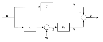
Figure 5: Differentially private filter approximation set-up.

We now generalize these mechanisms to the approximation set-up shown on Fig. 5. The previous mechanisms are recovered when $\mathcal{G}_{1}$ or $\mathcal{G}_{2}$ is the identity operator. To show that one can improve the utility of the mechanism with this set-up, consider the following choice of filters $\mathcal{G}_{1}$ and $\mathcal{G}_{2}$. Let $\mathcal{G}_{1}$ be a stable, minimum phase filter (hence invertible). Let $\mathcal{G}_{2}=\mathcal{G}\mathcal{G}_{1}^{-1}$. We call this particular choice the zero forcing equalization (ZFE) mechanism. To guarantee $(\epsilon,\delta)$-differential privacy, the noise $w$ is chosen to be white Gaussian with $\sigma=\kappa(\delta,\epsilon)\|\mathcal{G}_{1}\|_{2}$. The MSE for the ZFE mechanism is

$$e^{ZFE}_{mse}:= \lim_{T\to\infty}\frac{1}{T}\sum_{t=0}^{\infty}\mathbb{E}[\|(\mathcal{G}u)_{t}-(\mathcal{G}u+\mathcal{G}\mathcal{G}_{1}^{-1}w)_{t}\|^{2}_{2}]$$

$$= \lim_{T\to\infty}\frac{1}{T}\sum_{t=0}^{\infty}\mathbb{E}[\|(\mathcal{G}\mathcal{G}_{1}^{-1}w)_{t}\|_{2}^{2}]=\kappa(\epsilon,\delta)^{2}\|\mathcal{G}_{1}\|_{2}^{2}\|\mathcal{G}\mathcal{G}_{1}^{-1}\|^{2}_{2}.$$

Hence we are lead to consider the following problem

$$\min_{\mathcal{G}_{1}}\|\mathcal{G}_{1}\|_{2}^{2}\|\mathcal{G}\mathcal{G}_{1}^{-1}\|^{2}_{2}=\min_{\mathcal{G}_{1}}\frac{1}{4\pi^{2}}\int_{-\pi}^{\pi}|\mathcal{G}_{1}(e^{j\omega})|^{2}d\omega\int_{-\pi}^{\pi}\left|\frac{\mathcal{G}(e^{j\omega})}{\mathcal{G}_{1}(e^{j\omega})}\right|^{2}d\omega,$$

where the minimization is over the stable, minimum phase transfer functions $\mathcal{G}_{1}$.

Theorem 8.

We have, for any stable, minimum phase system $\mathcal{G}_{1}$,

$$e^{ZFE}_{mse}\geq\kappa(\epsilon,\delta)^{2}\left(\frac{1}{2\pi}\int_{-\pi}^{\pi}|\mathcal{G}(e^{j\omega})|d\omega\right)^{2}.$$

This lower bound on the mean-squared error of the ZFE mechanism is attained by letting $|\mathcal{G}_{1}(e^{j\omega})|^{2}=\lambda|\mathcal{G}(e^{j\omega})|$ for all $\omega\in[-\pi,\pi)$, where $\lambda$ is some arbitrary positive number. It can be approached arbitrarily closely by stable, rational, minimum phase transfer functions $\mathcal{G}_{1}$.

Proof.

By the Cauchy-Schwarz inequality, we have

$$\left(\int_{-\pi}^{\pi}|\mathcal{G}(e^{j\omega})|d\omega\right)^{2}=\left(\int_{-\pi}^{\pi}|\mathcal{G}_{1}(e^{j\omega})|\left|\frac{\mathcal{G}(e^{j\omega})}{\mathcal{G}_{1}(e^{j\omega})}\right|d\omega\right)^{2}\leq\int_{-\pi}^{\pi}|\mathcal{G}_{1}(e^{j\omega})|^{2}d\omega\int_{-\pi}^{\pi}\left|\frac{\mathcal{G}(e^{j\omega})}{\mathcal{G}_{1}(e^{j\omega})}\right|^{2}d\omega,$$

hence the bound. Moreover, equality is attained if and only if there exists $\lambda\in\mathbb{R}$ such that

$$|\mathcal{G}_{1}(e^{j\omega})|=\lambda\left|\frac{\mathcal{G}(e^{j\omega})}{\mathcal{G}_{1}(e^{j\omega})}\right|,\text{i.e., }|\mathcal{G}_{1}(e^{j\omega})|^{2}=\lambda|\mathcal{G}(e^{j\omega})|,\;\;\forall\omega\in\mathbb{R}.$$

To see that the bound can be approached using finite-dimensional filters, by Weierstrass theorem we can first approximate $|\mathcal{G}(e^{j\omega})|$ arbitrarily closely by a rational positive function $\hat{\mathcal{G}}$. We then set $\mathcal{G}_{1}$ to be the minimum-phase spectral factor of $\hat{\mathcal{G}}$. ∎

The MSE obtained for the best ZFE mechanism in Theorem 8 cannot be worse than the MSE for the scheme adding noise at the input, and is generally strictly smaller, since by Jensen’s inequality we have

$$\left(\int_{-\pi}^{\pi}|\mathcal{G}(e^{j\omega})|\frac{d\omega}{2\pi}\right)^{2}\leq\int_{-\pi}^{\pi}|\mathcal{G}(e^{j\omega})|^{2}\frac{d\omega}{2\pi}=\|\mathcal{G}\|_{2}^{2}.$$

In addition, the MSE of the ZFE mechanism is independent of the input signal $u$. However, a smaller error could be obtained with other schemes, in particular schemes that exploit some knowledge about the input signal. Note that once $\mathcal{G}_{1}$ is chosen, designing $\mathcal{G}_{2}$ is a standard equalization problem [31]. The name of the ZFE mechanism is motivated by the choice of trying to cancel the effect of $\mathcal{G}_{1}$ by using its inverse (zero forcing equalizer). Nonlinear components can be very useful as well. In particular if we add the hypothesis that the input signal is binary valued, as in [10, 30], we can modify the simple scheme adding noise at the input by including a detector $H$ in front of the system $\mathcal{G}$, namely, for $\hat{u}_{t}=u_{t}+w_{t}$,

$$H(\hat{u}_{t})=\begin{cases}1,\;\;\hat{u}_{t}\geq 1/2,\\ 0,\;\;\hat{u}_{t}<1/2.\end{cases}$$

This exploits the knowledge that the input signal is binary valued, preserves differential privacy by Theorem 1, and sometimes significantly improves the MSE, depending on other characteristics of the signal.

VI-A Exploiting Additional Public Knowledge

To further illustrate the idea of exploiting potentially available additional knowledge about the input signal, consider using a minimum mean squared error (MMSE) estimator for $\mathcal{G}_{2}$ rather than employing $\mathcal{G}\mathcal{G}_{1}^{-1}$, since the latter can significantly amplify the noise at frequencies where $\mathcal{G}_{1}$ is small. Let us assume that $\mathcal{G}_{1}$ is already chosen, e.g., according to Theorem 8 (this choice is not optimal any more if $\mathcal{G}_{2}$ is not $\mathcal{G}\mathcal{G}_{1}^{-1}$). Moreover, assume that that it is publicly known that $u$ is wide-sense stationary with mean and autocorrelation denoted

$$\mathbb{E}[u_{t}]=\mu,\;\;\mathbb{E}[u_{s}u_{t}]=:R_{u}[s-t].$$

From this data, the second order statistics of $y$ and $z$ on Fig. $1$ are also known, in particular

$$R_{z}=f*\tilde{f}*R_{u}+\sigma^{2}\delta,R_{yz}=g*\tilde{f}*R_{u},$$

where $\sigma^{2}=\kappa(\delta,\epsilon)^{2}\|\mathcal{G}_{1}\|_{2}^{2}$, $\delta$ is the impulse signal, $f$ is the impulse response of $\mathcal{G}_{1}$, and $\tilde{f}_{t}=f_{-t}$. We then design $\mathcal{G}_{2}$ to minimize the MSE

$$\mathbb{E}[|y_{t}-\hat{y}_{t}|^{2}].$$

For simplicity, consider the case where $\mathcal{G}_{2}$ is restricted to be a finite-impulse response filter, i.e.,

$$\hat{y}_{t}=(\mathcal{G}_{2}z)_{t}=\sum_{k=0}^{N}h_{k}z_{t-k},$$

where $N$ is the order of the filter. The vector $h=[h_{0},\ldots,h_{N}]^{T}$ is the solution of the Yule-Walker equations [32]

$$\begin{bmatrix}R_{z}[0]&R_{z}[1]&\ldots&R_{z}[N]\\ R_{z}[1]&R_{z}[0]&\ldots&R_{z}[N-1]\\ \vdots&\vdots&\vdots&\vdots\\ R_{z}[N]&\ldots&\ldots&R_{z}[0]\end{bmatrix}h=\begin{bmatrix}R_{yz}[0]\\ \vdots\\ R_{yz}[N]\end{bmatrix}$$

According to Theorem 1, differential privacy is preserved since the filter $\mathcal{G}_{2}$ only processes the already differentially private signal $z$. Even if the statistical assumptions turn out not to be satisfied by $u$, the privacy guarantee still holds and only performance is impacted.

Example 3.

Fig. 6 illustrates the differentially private output obtained by the MMSE mechanism approximating the filter $\mathcal{G}=1/(s(z)+0.05)$, with $s(z$) the bilinear transformation

$$s(z)=2\frac{1-z^{-1}}{1+z^{-1}}.$$

The input signal is binary valued and the privacy parameters are set to $\epsilon=\ln 3$, $\delta=0.05$. For this specific input, the empirical MSE of the ZFE is $5.8$, compared to $4.6$ for the MMSE mechanism. The simpler scheme with noise added at the input is essentially unusable, since its MSE is $\kappa(\delta,\epsilon)^{2}\|\mathcal{G}\|_{2}^{2}\approx 30.1$. Adding a detector reduces this MSE to about $17$.

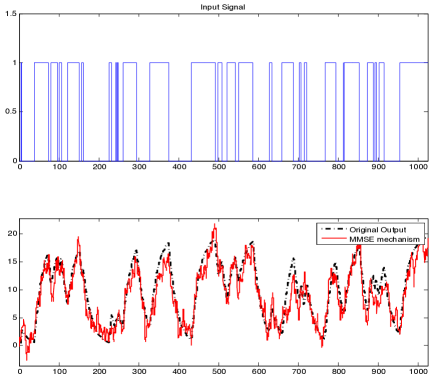
Figure 6: Sample path for the MMSE mechanism.

VI-B Related Work

Some papers closely related to the event filtering problem considered in this section are [10, 33, 11, 12]. As previously mentioned, [10, 33] consider an unstable filter, the accumulator. The techniques employed there are quite different, relying essentially on binary trees to keep track of intermediate calculations and reduce the amount of noise introduced by the privacy mechanism. Bolot et al. [12] extend this technique to the differentially private approximation of certain filters with monotonic, slowly decaying impulse response. In fact, this technique can be extended to general linear systems by using a state-space realization and keeping track of the system state at carefully chosen times in a binary tree. However, the usefulness of this approach seems to be limited for most practical stable filters, the resulting MSE being typically too large and the implementation of the scheme significantly more complex than for a simple recursive filter.

Finally, as with the MMSE estimation mechanism, one can try to use additional information about the input signals to calibrate the amount of noise introduced by the privacy mechanism. For example, if there exists a sparse representation of the signal in some basis (such as a Fourier or a wavelet basis), then one can try to perturb the representation coefficients in this alternate basis. For example, [33] perturbs the largest coefficients of the Discrete Fourier Transform of the signal. A difficulty with such approaches is that they are typically not causal and not recursive, requiring an amount of processing that increases with time.

VII Conclusion

We have discussed mechanisms for preserving the differential privacy of individual users transmitting time-varying signals to a trusted central server releasing sanitized filtered outputs based on these inputs. Decentralized versions of the mechanism of Section III can in fact be implemented in the absence of trusted server by means of cryptographic techniques [33]. We believe that research on privacy issues is critical to encourage the development of future cyber-physical systems, which typically rely on the users data to improve their efficiency. Numerous directions of study are open for dynamical systems, including designing better filtering mechanisms, and understanding design trade-offs between privacy or security and performance in large-scale control systems.

References

- [1] G. W. Hart, “Nonintrusive appliance load monitoring,” Proceedings of the IEEE, vol. 80, no. 12, pp. 1870–1891, December 1992.
- [2] A. Narayanan and V. Shmatikov, “Robust de-anonymization of large sparse datasets (how to break anonymity of the Netflix Prize dataset),” in Proceedings of the 2008 IEEE Symposium on Security and Privacy, 2008.
- [3] J. A. Calandrino, A. Kilzer, A. Narayanan, E. W. Felten, and V. Shmatikov, ““you might also like”: Privacy risks of collaborative filtering,” in IEEE Symposium on Security and Privacy, 2011.
- [4] B. Hoh, T. Iwuchukwu, Q. Jacobson, M. Gruteser, A. Bayen, J.-C. Herrera, R. Herring, D. Work, M. Annavaram, and J. Ban, “Enhancing privacy and accuracy in probe vehicle based traffic monitoring via virtual trip lines,” IEEE Transactions on Mobile Computing, 2011.
- [5] C. Dwork, F. McSherry, K. Nissim, and A. Smith, “Calibrating noise to sensitivity in private data analysis,” in Proceedings of the Third Theory of Cryptography Conference, 2006, pp. 265–284.
- [6] S. P. Kasiviswanathan and A. Smith, “A note on differential privacy: Defining resistance to arbitrary side information,” March 2008. [Online]. Available: http://arxiv.org/abs/0803.3946
- [7] C. Dwork, K. Kenthapadi, F. McSherry, I. M. M. Naor, and Naor, “Our data, ourselves: Privacy via distributed noise generation,” Advances in Cryptology-EUROCRYPT 2006, pp. 486–503, 2006.
- [8] A. Roth, “New algorithms for preserving differential privacy,” Ph.D. dissertation, Carnegie Mellon University, 2010.
- [9] C. Li, M. Hay, V. Rastogi, G. Miklau, and A. McGregor, “Optimizing linear counting queries under differential privacy,” in Principles of Database Systems (PODS), 2010.
- [10] C. Dwork, M. Naor, T. Pitassi, and G. N. Rothblum, “Differential privacy under continual observations,” in STOC’10, Cambridge, MA, June 2010.
- [11] T.-H. H. Chan, E. Shi, and D. Song, “Private and continual release of statistics,” ACM Transactions on Information and System Security, vol. 14, no. 3, pp. 26:1–26:24, November 2011.
- [12] J. Bolot, N. Fawaz, S. Muthukrishnan, A. Nikolov, and N. Taft, “Private decayed sum estimation under continual observation,” September 2011, http://arxiv.org/abs/1108.6123.
- [13] Z. Huang, S. Mitra, and G. Dullerud, “Differentially private iterative synchronous consensus,” in Proceedings of the CCS Workshop on Privacy in the Electronic Society (WPES), Raleigh, North Carolina, October 2012, to appear.
- [14] D. Varodayan and A. Khisti, “Smart meter privacy using a rechargeable battery: minimizing the rate of information leakage,” in Proceedings of the IEEE International Conference on Acoustics, Speech, and Signal Processing, Prag, Czech Republic, 2011.
- [15] L. Sankar, S. R. Rajagopalan, and H. V. Poor, “A theory of privacy and utility in databases,” Princeton University, Tech. Rep., February 2011.
- [16] A. Blum, C. Dwork, F. McSherry, and K. Nissim, “Practical privacy: the SuLQ framework,” in Proceedings of the twenty-fourth ACM SIGMOD-SIGACT-SIGART symposium on Principles of database systems (PODS), New York, NY, USA, 2005, pp. 128–138.
- [17] C. Dwork, “Differential privacy,” in Proceedings of the 33rd International Colloquium on Automata, Languages and Programming (ICALP), ser. Lecture Notes in Computer Science, vol. 4052. Springer-Verlag, 2006.
- [18] R. M. Dudley, Real Analysis and Probability, 2nd ed. Cambridge University Press, 2002.
- [19] T. M. Cover and J. A. Thomas, Elements of Information Theory. New York, NY: John Wiley and Sons, 1991.
- [20] L. Breiman, Probability, ser. Classics in Applied Mathematics. SIAM, 1992.
- [21] A. van der Schaft, L2-gain and passivity techniques in nonlinear control. Springer Verlag, 2000.
- [22] E. Shi, T.-H. H. Chan, E. Rieffel, R. Chow, and D. Song, “Privacy-preserving aggregation of time-series data,” in Proceedings of 18th Annual Network and Distributed System Security Symposium (NDSS 2011), February 2011.
- [23] B. D. O. Anderson and J. B. Moore, Optimal Filtering. Dover, 2005.
- [24] R. E. Skelton, T. Iwasaki, and K. Grigoriadis, A Unified Algebraic Approach to Linear Control Design. Taylor and Francis, 1998.
- [25] C. Scherer, P. Gahinet, and M. Chilali, “Multiobjective output-feedback control via LMI optimization,” IEEE Transactions on Automatic Control, vol. 42, no. 7, pp. 896–911, July 1997.
- [26] X. Sun, L. Munoz, and R. Horowitz, “Mixture Kalman filter based highway congestion mode and vehicle density estimator and its application,” in Proceedings of the American Control Conference, July 2004, pp. 2098–2103.
- [27] M. Gruteser and D. Grunwald, “Anonymous usage of location-based services through spatial and temporal cloaking,” in ACM MobiSys, 2003.
- [28] R. Shokri, J. Freudiger, M. Jadliwala, and J.-P. Hubaux, “A distortion-based metric for location privacy,” in Proceedings of the CCS Workshop on Privacy in the Electronic Society (WPES), 2009.
- [29] R. Shokri, C. Troncoso, C. Diaz, J. Freudiger, and J.-P. Hubaux, “Unraveling an old cloak: -anonymity for location privacy,” in ACM Workshop on Privacy in the Electronic Society (WPES). ACM, 2010.
- [30] T.-H. H. Chan, E. Shi, and D. Song, “Private and continual release of statistics,” University of California at Berkeley, Tech. Rep., 2010.
- [31] J. Proakis, Digital Communications. McGraw-Hill, 2000.
- [32] H. V. Poor, An Introduction to Signal Detection and Estimation, 2nd ed. Springer, 1994.
- [33] V. Rastogi and S. Nath, “Differentially private aggregation of distributed time-series with transformation and encryption,” in Proceedings of the ACM Conference on Management of Data (SIGMOD), Indianapolis, IN, June 2010.