Quantum Trajectory Approach to Molecular Dynamics Simulation with Surface Hopping

Abstract

The powerful molecular dynamics (MD) simulation is basically based on a picture that the atoms experience classical-like trajectories under the exertion of classical force field determined by the quantum mechanically solved electronic state. In this work we propose a quantum trajectory approach to the MD simulation with surface hopping, from an insight that an effective “observation” is actually implied in the MD simulation through tracking the forces experienced, just like checking the meter’s result in the quantum measurement process. This treatment can build the nonadiabatic surface hopping on a dynamical foundation, instead of the usual artificial and conceptually inconsistent hopping algorithms. The effects and advantages of the proposed scheme are preliminarily illustrated by a two-surface model system.

A full quantum mechanical treatment for molecular dynamics (MD) would break down along the increase of atomic degrees of freedom. As a result, in practice the MD technique based on an assumption that atomic motions are governed by classical mechanics has proved to be a very powerful tool MD-1 ; MD-2 ; MD-4 ; Tul98a ; Bar11 . The MD simulations usually rely on the Born-Oppenheimer (BO) approximation, which decouples the electronic and atomic motions. That is, the atoms experience classical-like trajectories under the exertion of appropriate classical force field, which is determined by a single potential energy surface (PES) associated with a single electronic state. On the other aspect, the electronic states are solved from the time-independent Schrödinger equation for a series of atomic geometries (configurations).

In many situations, however, when the energy separation of different PESs becomes comparable with the magnitude of the nonadiabatic coupling (typically in the proximity of conical intersection, see Fig. 1), the BO approximation may often fail. In this case, since each nondegenerate electronic state defines a distinct BO PES, a transition between electronic states would change, often drastically, the forces experienced by the atoms. Proper account for this nonadiabatic effect is of crucial importance in practice. The treatment of nonadiabatic effects in MD has a long history. The most widely applied include the so-called “Ehrenfest” or “time-dependent-Hartree mean-field (TDHMF)” approach Rat82 ; Mic83 ; Tul98a ; Fri05 , the “trajectory surface-hopping (TSH) methods Nik68 ; Tul71 ; Mi72 ; Kun79 ; Bla83 ; Mi83 ; Tul90 ; Tul94 , and their mixed schemes Kun91 ; Zhu04 ; Jan09 . The former approach views that the electronic wavefunction might in general be a linear combination of the BO adiabatic functions, the atomic effective potential is thus calculated by averaging the electronic Hamiltonian over such wavefunction, while the BO adiabatic functions are determined self-consistently with the atomic trajectory. The TSH, a more appropriate methodology for dynamics propagation of nonadiabatic systems, is however based on an insight that the trajectories should split into branches, i.e., each trajectory should be on one state or another, not somewhere in between. And, the trajectories distribution is achieved by allowing hops between surfaces according to some probability distribution.

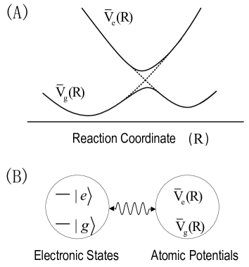
Figure 1: (A) Schematic atomic potentials in terms of adiabatic (solid) and diabatic (dashed) representations for the electronic ground and first excited states along the reaction coordinate. (B) Measurement analogy by dividing the molecular system into two subsystems, and regarding the atomic part as a “measurement apparatus” which continuously probes the distinct electronic states by the experienced distinct forces.

A variety of trajectory-based methods have been developed. Among them, the most typical one is Tully’s fewest switches surface hopping (FSSH) algorithm Tul90 . This algorithm is based on the following insights/arguments: (i) The atomic trajectories determine the probabilities of electronic transitions and the electronic transitions, in turn, strongly influence the forces governing the trajectories. (ii) The atoms evolve on individual single PES and the nonadiabatic effects are included by allowing hopping from one PES to another according to the weight of the respective electronic state. In the past two decades, stimulated by Tully’s work, a variety of variants of the FSSH algorithm and a large number of applications have been carried out Cok9192 ; Cok93 ; Tul9495 ; Ros97 ; Tul98 ; Fri91a ; Fri94 ; Las08a ; Las08b ; Fab08 ; Hay09 .

Nevertheless, the coherence between states, maintained in the FSSH algorithm is usually wrong because of the independent trajectory approach (see the recent review Bar11 ). The underlying conceptual difficulty can be further understood as follows. In the FSSH algorithm, the nonadiabatic effect is treated by allowing hopping from one PES to another, with the hopping probability determined by the weight change of the respective electronic states in quantum superposition. Physically, however, the atomic classical trajectory along a specific individual PES implies that it must collapse the electronic state onto the corresponding BO wavefunction, according to the distinct classical force experienced. In other words, we can no longer treat the electronic state in a quantum superposition of the many different components, as in contrast proposed in the FSSH approach Tul90 . As shown in Fig. 1(B), through an analogy with quantum measurement or with the more popular Schrödinger’s Cat paradox, the FSSH algorithm simply means that we are still treating the radioactive decay in a quantum superposition state, while having found the Cat definitely “alive” or “dead”.

In this work, rather than designing certain wiser algorithms for the TSH probability, we would like to view the problem in an alternative way and accordingly propose a quantum trajectory approach to the MD simulation. That is, we are able to develop a self-consistent in physics and hopefully highly implementable stochastic MD scheme, which quite naturally renders the TSH in the most fundamental notion of quantum jump.

Formulation.— For the purpose to be clear soon, we introduce the electronic Hamiltonian by subtracting the atomic kinetic energy from the total Hamiltonian as

$$H_{el}(r,\textbf{R})=-\sum_{j}\frac{\hbar^{2}}{2m_{j}}\nabla_{j}^{2}+V(r,\textbf{R}).$$ (1)

Here, the first term describes the kinetic energy of electrons. We use $r$ denoting all the electronic coordinates, i.e., $r\equiv\{r_{j};j=1,2,\cdots\}$. And, formally, R denotes the atomic configuration.

We expand the electronic wavefunction by a set of known basis functions, $\Psi(r,\textbf{R})=\sum_{j}c_{j}(t)\phi_{j}(r,\textbf{R})$. In principle, $\{\phi_{j}(r,\textbf{R})\}$ can be any electronic basis functions, while in practice it would be convenient to chose them as the Born-Oppenheimer adiabatic wavefunctions. That is, $H_{el}(r,\textbf{R})\phi_{j}(r,\textbf{R})=\varepsilon_{j}(\textbf{R})\phi_{j}(r,\textbf{R})$, which means that $\phi_{j}(r,\textbf{R})$ are the instantaneous eigenstates of $H_{el}(r,\textbf{R})$, for a given $\textbf{R}\equiv\textbf{R}(t)$. These basis wavefunctions, together with the corresponding eigen-energies $\varepsilon_{j}(\textbf{R})$, are the standard output of the usual quantum chemistry computation. Using the selected basis functions, we further introduce

$$V_{jk}(\textbf{R}) = \langle\phi_{j}(r,\textbf{R})|H_{el}(r,\phi_{j}(r,\textbf{R}))|\phi_{k}(r,\textbf{R})\rangle,$$ (2)

$$\textbf{d}_{jk}(\textbf{R}) = \langle\phi_{j}(r,\textbf{R})|\nabla_{\textbf{R}}|\phi_{k}(r,\textbf{R})\rangle.$$ (3)

Obviously, for the BO adiabatic basis, $V_{jk}(\textbf{R})$ is diagonal, $V_{jk}(\textbf{R})=\varepsilon_{j}(\textbf{R})\delta_{jk}\equiv\bar{V}_{j}(\textbf{R})\delta_{jk}$. Each $\bar{V}_{j}(\textbf{R})$ is known as the BO potential energy surface (PES). The quantity $\textbf{d}_{jk}(\textbf{R})$ characterizes nonadiabatic coupling between the ($j$th and $k$th) PESs, which has an effect of driving surface hopping. This can be seen more clearly by the following. The coherent electronic evolution is governed by the Schrödinger equation $i\hbar\dot{\Psi}=H_{el}\Psi$, which results in a set of coupled equations for $c_{j}(t)$

$$i\hbar\dot{c}_{j} = \sum_{k}\left[V_{jk}(\textbf{R})-i\hbar\dot{\textbf{R}}\cdot\textbf{d}_{jk}(\textbf{R})\right]c_{k}$$ (4)

$$\equiv \sum_{jk}\tilde{H}_{jk}(\textbf{R})c_{k}.$$

In this expression, we can understand $\tilde{H}_{jk}(\textbf{R})$ as an effective Hamiltonian matrix in the selected basis, which straightforwardly describes the evolution of the state amplitudes $c_{j}(t)$. In terms of a projective operator form, the effective Hamiltonian can be expressed as $\tilde{H}(\textbf{R})=\sum_{jk}\tilde{H}_{jk}(\textbf{R})|\phi_{j}(\textbf{R})\rangle\langle\phi_{k}(\textbf{R})|$. Using the property $\textbf{d}^{*}_{jk}(\textbf{R})=-\textbf{d}_{kj}(\textbf{R})$, one can prove that $\tilde{H}(\textbf{R})$ is Hermitian, as it should be. Moreover, corresponding to the BO adiabatic basis, we have even simpler results: $\tilde{H}_{jj}(\textbf{R})\equiv\varepsilon_{j}(\textbf{R})$; and $\tilde{H}_{jk}(\textbf{R})\equiv\Omega_{jk}(\textbf{R})=-i\hbar\dot{\textbf{R}}\cdot\textbf{d}_{jk}(\textbf{R})$, if $j\neq k$. In this way, we see that it is the product of $\dot{\textbf{R}}$ and $\textbf{d}_{jk}(\textbf{R})$ that characterizes the nonadiabatic coupling between the BO potential surfaces.

It was merely based on Eq. (4), which describes the quantum mechanical evolution of the superposition amplitudes of electronic states, that the highly celebrated FSSH algorithm was proposed Tul90 , with the following central idea. From the “normalized” population change of the electronic state $|\phi_{j}(\textbf{R})\rangle$, defined as $p_{j}(t)=[|c_{j}(t)|^{2}-|c_{j}(t+\Delta t)|^{2}]/|c_{j}(t)|^{2}$, one performs a standard Monte-Carlo choice (with this probability $p_{j}(t)$) to determine whether or not a hopping event should take place, from the BO potential surface $\bar{V}_{j}(\textbf{R})$ to another one.

Intuitively, this looks indeed a promising algorithm, since the BO potential surface $\bar{V}_{j}(\textbf{R})$ is anyhow associated with the electronic state $|\phi_{j}(\textbf{R})\rangle$, one can then conclude that the change of the electronic occupation probability must imply a surface-hopping event occurred. Nevertheless, in each single realization of MD trajectory, the atomic motion experiences a series of distinct PESs (but not their weighted superposition), together with successive hopping between them. Based on the entanglement-type correlation between the electronic states and the atomic PESs, see Fig. 1(B), the classical trajectory treatment for the atomic motion must collapse the electronic state to an individual one, with the result determined by the classical force experienced by the atoms. In other words, we can no longer inappropriately maintain the electronic state in a quantum superposition of two (or many) different components $|\phi_{j}(\textbf{R})\rangle$, as in contrast assumed in the FSSH approach Tul90 . In essence, using the term of Schrödinger’s Cat paradox, the mixed quantum-classical FSSH treatment is equivalent to treating the radioactive decay still in “quantum superposition”, while one has definitely found the Cat “alive” or “dead”.

In order to eliminate the above inconsistency in the FSSH algorithm, we propose that one should apply a measurement-based description to the electronic state evolution, instead of using the R-dependent Schrödinger equation. Indeed, since R enters the Schrödinger equation, this partly accounts for the effect of the atomic motion on the electronic state evolution. But this is not enough. Actually, the atomic motion is continuously getting the state information of the electrons, via the correlation between the PES and the electronic state. As a result, in addition to involving “R” as an external parameter in the electronic Schrödinger equation, one should at the same time account for the backaction of the electronic-state information gain. This means that the atomic motion is in essence making a continuous quantum measurement on the electronic state. The distinct “force” experienced by the atomic trajectory motion, effectively, plays the same role as the meter’s output in quantum measurement process.

After the above conceptual preparation, we can then apply the established quantum trajectory equation (QTE) to account for the backaction effect owing to state information gain as follows WM10

$$\dot{\rho} = -\frac{i}{\hbar}\left[\tilde{H}(\textbf{R}),\rho\right]+\sum_{j}\Gamma_{\phi j}{\cal D}\left[M_{j}(\textbf{R})\right]\rho$$ (5)

$$+\sum_{j}\sqrt{\Gamma_{\phi j}}{\cal H}\left[M_{j}(\textbf{R})\right]\rho~{}\xi_{j}(t).$$

Here, $\rho$ is the electronic state density matrix, with elements $\rho_{jk}$. The diagonal elements describe population probabilities on the BO states, while the off-diagonal elements describe quantum coherence between them. Note that, on the left hand side of Eq. (5), we have made a convention that $\dot{\rho}$ represents $\sum_{jk}\dot{\rho}_{jk}|\phi_{j}(\textbf{R})\rangle\langle\phi_{k}(\textbf{R})|$, but not $\frac{d}{dt}[\sum_{jk}\rho_{jk}|\phi_{j}(\textbf{R})\rangle\langle\phi_{k}(\textbf{R})|]$. Accordingly, $\tilde{H}(\textbf{R})$ in the above QTE is the effective Hamiltonian defined in Eq. (4).

In Eq. (5), the measurement operator, $M_{j}(\textbf{R})=|\phi_{j}(\textbf{R})\rangle\langle\phi_{j}(\textbf{R})|$, corresponds to an identification (discrimination) to the electronic state $\phi_{j}(\textbf{R})$ by the atomic motion. It is well known that any state discrimination will destroy the quantum coherence (the quantum superposition). This effect is described by the second term in Eq. (5), with the dephasing rate $\Gamma_{\phi j}$ corresponding to discrimination of the state $\phi_{j}(\textbf{R})$. Here the Lindblad-type superoperator means, ${\cal D}[M_{j}]\rho=M_{j}\rho M_{j}^{\dagger}-\frac{1}{2}\{M_{j}^{\dagger}M_{j},\rho\}$. Finally and very importantly, the last term in Eq. (5) accounts for the effect of state information gain. The involved superoperator, more explicitly, is defined as ${\cal H}[M_{j}]\rho=M_{j}\rho+\rho M_{j}^{\dagger}-\langle M_{j}+M_{j}^{\dagger}\rangle\rho$, where $\langle M_{j}+M_{j}^{\dagger}\rangle\equiv{\rm Tr}[(M_{j}+M_{j}^{\dagger})\rho]$. $\xi_{j}(t)$ are the Gaussian stochastic noises, satisfying the ensemble average property ${\rm E}[\xi_{j}(t)\xi_{k}(t^{\prime})]=\delta_{jk}\delta(t-t^{\prime})$. Notice that the last term in Eq. (5) is not originated from any external noise, but from an intrinsic stochastic collapse (quantum jump) associated with “observation”, i.e., the quantum measurement postulate.

Applying Eq. (5) in a strong observation regime (with large $\Gamma_{\phi j}$), one can generate the desired TSH picture. That is, the large $\Gamma_{\phi j}$ correspond to MD simulation under distinct forces. Then, under the influence of the atomic trajectory motion, the nonadiabatic coupling will drive a series of stochastic jumps between the BO states. This is nothing but the desired “surface hopping” behavior which can be generated, in the existing schemes, only by constructing various hopping “algorithms”, non-dynamically.

Alternatively, applying Eq. (5) in a weaker observation regime (with smaller $\Gamma_{\phi j}$), while the atomic motion propagates along a single PES away from the level-crossing area, the Ehrenfest-type mean field approach is restored in the proximity of the level-crossing area. That is, by computing the potential energy via $\bar{V}(\textbf{R})={\rm Tr}[H_{el}(r,\textbf{R})\rho(t)]$, the effect of quantum superposition of the BO potential surfaces is taken into account. In our opinion, this effect should exist there. Using the term of quantum measurement, this simply corresponds to an incomplete observation in the level crossing area where the atomic motion, particularly in the case of strong nonadiabatic coupling, does not fully distinguish which potential surface, but only experiences a mixed force. We believe that applying the proposed approach to the above regime is a valuable extension of the hybrid TSH-TDHMF scheme.

Illustrative Demonstration.— Below we illustrate how the approach proposed above can generate the TSH behavior, dynamically (or physically in essence), instead of using the probability algorithms to generate the “hopping” events. For simplicity, we restrict our demonstration to a one-dimensional (1D) two-surface example. Because of the 1D nature, in what follows we denote “R” simply by “$R$”. To be specific, we model the two BO potential surfaces as schematically shown in Fig. 2(A). For $|R-R_{0}|>a$, we assume $\varepsilon_{2}(R)-\varepsilon_{1}(R)=\alpha|R-R_{0}|$; while for $|R-R_{0}|\leq a$, the adiabatic energy difference is a constant, $\varepsilon_{2}(R)-\varepsilon_{1}(R)=\Delta$. Here, the scale of the level-crossing area is determined by $a=\Delta/\alpha$. Rather than a real MD simulation, following the Landau-Zener model, we assume a constant speed for the atomic motion, i.e., $R(t)=vt$. Moreover, the nonadiabatic coupling is parameterized as $\tilde{H}_{12}=(\tilde{H}_{21})^{*}=-i\hbar v\beta\equiv-i\hbar\Omega$, from an assumption of $\dot{R}\cdot d_{12}(R)=v\beta$.

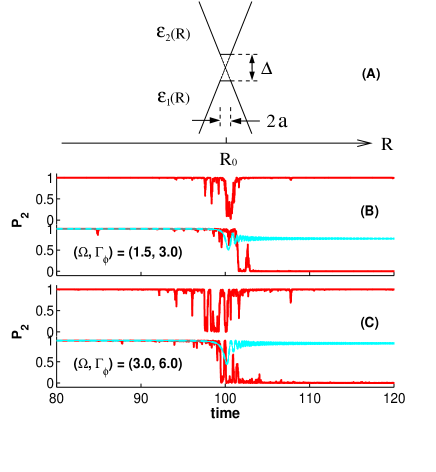
Figure 2: Demonstration of the surface-hopping behavior. (A): The model we used in our numerical simulation. (B) and (C): Four representative trajectories (red curves) from two groups of parameters, while the cyan curves stand for the results of $\Gamma_{\phi}=0$ in the absence of “observation”. Other parameters: $\Delta=1.0$ and $\alpha=10$. In the simulation (also in Fig. 3 and in the main-text discussion) we assume $\Gamma_{\phi 1}=\Gamma_{\phi 2}\equiv\Gamma_{\phi}$.

In Fig. 2(B) and (C) we display some representative quantum trajectories. First, we notice that the nonadiabatic coupling (with constant magnitude “$\Omega$”) can cause efficient transitions largely in the proximity of the conical intersection area, because of the relatively small energy separation between the PESs. Also, in the whole range, Eq. (5) will give a quantum mechanically pure (but not unitary) evolution for the electronic state. Fig. 2(B) corresponds to a situation with relatively weak coupling and weak observation. In this case, in the intersection area the electronic state consists of a superposition of the BO basis states. Using this state to calculate the atomic forces, desirably, should be an extension of the usual mean-field approach. However, if we increase $\Gamma_{\phi}$ further, as shown in Fig. 2(C), in the proximity of the central level-crossing area the sharp “surface hopping” behavior will appear eventually.

We emphasize in this context that, very importantly, even for a weak strength $\Gamma_{\phi}$ the trajectory will gradually and stochastically collapse onto one of the energy surfaces. This is in sharp contrast with the prediction of the Schrödinger equation. In that case, the state will remain in quantum superposition, after the evolution passes through the central intersection area. We demonstrate this feature by the cyan curves in both Fig. 2(B) and (C), where we see that the final state is indeed in superposition. However, a continuous “observation” will collapse the state, gradually, onto one of the basis states, either $|\phi_{1}\rangle$ or $|\phi_{2}\rangle$. Then the desired picture of trajectory propagation along a single energy surface is generated, by this dynamical and physical means.

In practice, to compare the stochastic MD simulation with experiments, one should ensemble-average the stochastic trajectories. For the assumed constant speed of atomic motion, the trajectory distribution can be simply predicted by averaging the QTE first. This can be done easily by removing the last (unraveling) term in Eq. (5) and remaining only the first two terms. We actually obtain the usual master equation. Then, from the density matrix, we get the probabilities $p_{1}(t)=\rho_{11}(t)$ and $p_{2}(t)=\rho_{22}(t)$, which give the distribution ratio of the atomic trajectories in the asymptotic limit ($t\rightarrow\infty$). We should note that, however, in practical MD simulations one cannot average first Eq. (5), since for different trajectories the stochastic atomic forces experienced would be different. Obviously, this feature cannot be captured by the averaged master equation. In other words, the averaged master equation does not allow us to correctly compute the atomic forces, we are then unable to propagate the atomic motion based on Newton’s law. This is the reason that in literature, when one attempts to introduce decoherence, the master equation approach does not work.

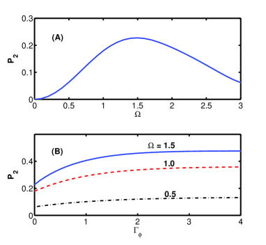
Figure 3: Nonadiabatic transition probability from the initial state $|\phi_{1}(R_{-\infty})\rangle$ to the final one $|\phi_{2}(R_{\infty})\rangle$. $R_{\mp\infty}$ represent the initial and final asymptotic reaction coordinates. This probability indicates the distribution of the final “products”. (A) Dependence on the nonadiabatic coupling strength in the absence of dephasing ($\Gamma_{\phi}=0$). (B) Dephasing effect on the transition probability. Parameters: $\Delta=1.0$ and $\alpha=10$.

In Fig. 3(A), we show the dependence of the nonadiabatic transition on the coupling strength. We take $\Gamma_{\phi}=0$ in order to reveal this mere dependence more clearly. We observe a turnover behavior, with an optimal nonadiabatic coupling to make the transition reach maximum. This feature indicates, in some counterintuitive manner, that a faster atomic motion may not necessarily enhance the transition probability. This behavior differs somehow from the prediction of the Landau-Zener formula, since that formula will give a larger transition probability for a faster speed. The reason is that, here, in the adiabatic BO basis, the faster atomic motion will enhance the nonadiabatic coupling between the energy surfaces, while in the Landau-Zener model, expressed in a diabatic basis, the passage speed across the intersection area has no such effect .

In Fig. 3(B), we show the decoherence effect on the nonadiabatic transition. Here we observe a decoherence-enhanced transition behavior. But, this feature is not universal. It only corresponds to a weak dynamic tunneling regime. Actually, not shown in Fig. 3(B), if we tune the coupling strength into an intermediate tunneling regime, a turnover behavior can appear, whereas a decoherence-suppressed transition will take place in strong tunneling regime. We also observe that, if an efficient coupling persists in the intersection area for longer time, the decoherence will result in a final equal occupation on the both energy surfaces, as shown by the curve with $\Omega=1.5$ in Fig. 3(B).

Finally, we remark that a decoherence in the TSH should arise because the MD simulation is propagated along a single trajectory determined by the gradients for an specific electronic state. In this propagation, the amplitudes of all other states are artificially restricted to be also propagated along the same trajectory, even though the gradients of these other states would dissipate these amplitudes along other directions. This effect has been discussed in detail and corrections to it have been proposed Sch96 ; Tha98 ; Zhu05 ; Gra07 ; Gra10 . For instance, in Ref. Gra07 , it was shown that the divergence between occupation and average population is caused by the missing decoherence, and that this discrepancy can be eliminated if the decoherence corrections are incorporated.

Acknowledgments.— We thank Jiushu Shao, Zhenggang Lan and Sheng Meng for stimulating discussions. This work was supported by the Major State Basic Research Project of China (No. 2011CB808502 & 2012CB932704) and the NNSF of China (No. 101202101 & 10874176).

Appendix A Measurement Interpretation

In this appendix we present a further discussion to relate the stochastic MD simulation with quantum measurement. As mentioned in the main text, we can divide the whole system into two coupled electronic and atomic subsystems, as shown in Fig. 1(B). Under the BO approximation, the relatively heavy and slowly moving atomic subsystem largely experiences a classical-like trajectory motion. Therefore, the atomic subsystem looks very like a measurement meter, which is continuously “measuring” the electronic states by its experienced distinct forces. In this context, the PES (or force) is the meter’s output (measurement result), from which the electronic state is inferred.

In a more heuristic manner, we may relate the problem to the paradox of Schrödinger’s Cat. As illustrated in Fig. 1(B), we assume two electronic states, $|g\rangle$ and $|e\rangle$. Accordingly, we have two PESs, $\bar{V}_{g}(R)$ and $\bar{V}_{e}(R)$, which correspond to the Cat states “alive” and “dead”. If we insist on regarding the whole system as a closed one, we will arrive to a (quantum) superposition of $\bar{V}_{g}(R)$ and $\bar{V}_{e}(R)$, exactly as the superposition of “alive” and “dead” states in the Cat paradox. But, as is well known, the Cat paradox can be resolved only by a neglect of the large number of microscopic degrees of freedom of the Cat and the surrounding environment. It is merely this treatment that can result in the emergence of classicality which shows the Cat in a state of either “alive” or “dead”, but not in between. We then arrive to two statements: (i) In the semi-classical stochastic MD simulation, the essential picture of classical trajectory and surface hopping has implied an incorporation of certain external environment and an effective observation. For a closed quantum system, there is no way to generate the jump (hopping) behavior. (ii) We hypothesize that the TSH-based MD simulations are more appropriate for many-atom system in condensed phase. For an “isolated (clean)” few-atom system, a full quantum mechanical simulation should be required.

In the TSH-MD simulations, we can imagine that the “observation” is realized through tracking the forces experienced, just like checking the meter’s result in the quantum measurement process. Together with the quantum nonadiabatic coupling, successive jumps then appear, exactly like in the continuous measurement of a driving systemWM10 . Moreover, this approach is quite versatile. For instance, it can describe the possible “partial” hopping behavior. That is, when the atomic motion passes through the conical intersection region, the atoms may not be able to resolve the experienced force from which PES. In this case, the resultant state is still in quantum superposition. However, the state evolution should obey the quantum trajectory equation, Eq. (5), but not the Schrödinger equation. We believe that this treatment is a valuable extension of the hybrid TSH-TDHMF approachKun91 ; Zhu04 ; Jan09 .

References

- (1) A. R. Leach, Molecular Modeling: Principles and Applications (2nd Ed., Pearson Education Limited, England, 2001).
- (2) D. Marx, J. Hütter, Ab Initio Molecular Dynamics: Basic Theory and Advanced Methods (Cambridge University Press, Cambridge, England, 2009).
- (3) G. Stock, M. Thoss, Adv. Chem. Phys. 131, 243-375 (2005).
- (4) J. C. Tully, Faraday Discuss 110, 407 C419 (1998).
- (5) M. Barbatti, Advanced Review 1, 620 (2011).
- (6) R. B. Gerber, V. Buch, and M. A. Ratner, J. Chem. Phys. 77, 3022 (1982).
- (7) D. A. Micha, J. Chem. Phys. 78, 7138 (1983).
- (8) X. Li, J. C. Tully, H. B. Schlegel, and M. J. Frisch, J. Chem. Phys. 123, 084106 (2005).
- (9) E. E. Nikitin, Theory of non-adiabatic transitions. Recent developments of the Landau-Zener (linear) model. In: H. Hartmann, J. Heidberg, H. Heydtmann, G. H. Kohlmaier, eds. Chemische Elementarprozesse (Berlin: Springer-Verlag; 1968, 43 C77).
- (10) J. C. Tully, P. K. Preston, J. Chem. Phys 55, 562 (1971).
- (11) W. H. Miller and T. F. George, J. Chem. Phys. 56, 5637 (1972).
- (12) P. J. Kuntz, J. Kendrick, and W. N. Whitton, Chem. Phys. 38, 147(1979).
- (13) N. C. Blais and D. G. Truhlar, J. Chem. Phys. 79, 1334 (1983).
- (14) D. P. Ali and W. H. Miller, J. Chem. Phys. 78, 6640 (1983).
- (15) J. C. Tully, J. Chem. Phys. 93, 1061 (1990).
- (16) S. Hammes-Schiffer and J. C. Tully, J. Chem. Phys. 101, 4657 (1994).
- (17) P. J. Kuntz, J. Chem. Phys. 95, 141 (1991).
- (18) C. Zhu, A. W. Jasper, and D. G. Truhlar, J. Chem. Phys. 120, 5543 (2004).
- (19) I. Janecek, S. Cintava, D. Hrivnak, R. Kalus, M. Farnik, and F. X. Gadea, J. Chem. Phys. 131, 114306 (2009).
- (20) B. Space and D. F. Coker, J. Chem. Phys. 94, 1976 (1991); J. Chem. Phys. 96, 652 (1992).
- (21) D. F. Coker, in Computer Simulations in Chemical Physics, edited by M.P. Allen and D. J. Tildesley (Kluwer, Netherlands, 1993), pp. 315 C377.
- (22) S. Hammes-Schiffer and J. C. Tully, J. Chem. Phys. 101, 4657 (1994); J. Phys. Chem. 99, 5793 (1995).
- (23) O. V. Prezhdo, and Peter J. Rossky, J. Chem. Phys. 107, 825 (1997).
- (24) D. S. Sholl and J. C. Tully, J. Chem. Phys. 109, 7702 (1998).
- (25) F. A. Webster, P. J. Rossky, and R. A. Friesner, Comp. Phys. Commun. 63, 494 (1991).
- (26) F. A. Webster, E. T. Wang, P. J. Rossky, and R. A. Friesner, J. Chem. Phys. 100, 4835 (1994).
- (27) C. Lasser and T. Swart, J. Chem. Phys. 129, 034302 (2008).
- (28) C. F. Kammerer and C. Lasser, J. Chem. Phys. 128, 144102 (2008).
- (29) E. Fabiano, G. Groenhof G, and W. Thiel, Chem. Phys. 351, 111 (2008).
- (30) S. Hayashi, E. Taikhorshid, and K. Schulten, Biophys. J. 96, 403 (2009).
- (31) H. M. Wiseman and G. J. Milburn, Quantum Measurement and Control (Cambridge University Press, 2010).
- (32) B. J. Schwartz, E. R. Bittner, O. V. Prezhdo, and P. J. Rossky, J. Chem. Phys. 104, 5942 (1996).
- (33) M. Thachuk, M. Y. Ivanov, and D. M. Wardlaw, J. Chem. Phys. 109, 5747 (1998).
- (34) C. Zhu, A. W. Jasper, and D. G. Truhlar, J. Chem. Theor. Comput. 1, 527 (2005).
- (35) G. Granucci, M. Persico, J. Chem. Phys. 126, 134114 (2007).
- (36) G. Granucci, M. Persico, and A. Zoccante, J. Chem. Phys. 133, 134111 (2010).