On the Statistical Efficiency of Multi-Task Learning of Gaussian Graphical Models
Abstract
In this paper, we present multi-task structure learning for Gaussian graphical models. We analyze the sufficient number of samples for the correct recovery of the support union and edge signs. We also analyze the necessary number of samples for any conceivable method by providing information-theoretic lower bounds. We compare the statistical efficiency of multi-task learning versus that of single-task learning. For experiments, we use a block coordinate descent method that is provably convergent and generates a sequence of positive definite solutions. We provide experimental validation on synthetic data as well as on two publicly available real-world data sets, including functional magnetic resonance imaging and gene expression data.
1 Introduction
Structure learning aims to discover the topology of a probabilistic graphical model that accurately represents a given data set. Accuracy of representation is measured by the likelihood that the model explains the observed data. One challenge faced by structure learning is that the number of possible structures is super-exponential in the number of variables. A computationally tractable method, -norm regularization, has been successfully used for learning sparse structures, cf., [Meinshausen and Bühlmann, 2006, Banerjee et al., 2006, Yuan and Lin, 2007]. Sparse structures are easier to be interpreted, given the small number of edges. Furthermore, sparsity guarantees the correct recovery of the edges [Ravikumar et al., 2011].
In several application domains, structure learning is very useful for analyzing data sets for which probabilistic dependencies are not known apriori. For instance, these techniques allow for modeling interactions between brain regions as well as the interactions between genes. Suppose that we want to learn the structure of interactions for one group under analysis (e.g., a specific collection site or a specific cancer type). We can expect that the interaction patterns of two groups are not exactly the same. On the other hand, when learning the structure for one group, we would like to use evidence from other groups as side information in our learning process. This becomes more important in settings with limited amount of data and high variability, such as in functional magnetic resonance imaging (fMRI) as well as in gene expression data. Multi-task learning allows for a more efficient use of training data which is available for multiple related tasks.
In this paper, we consider the multi-task structure learning problem, which generalizes the learning of sparse Gaussian graphical models to the multi-task setting by replacing the -norm regularization with an -norm, also known as the simultaneous prior [Turlach et al., 2005, Tropp, 2006] for , or the group-sparse prior [Yuan and Lin, 2006, Meier et al., 2008] for . Here, we assume that . This includes two specific instances previously evaluated experimentally: [Honorio and Samaras, 2010] when , and [Varoquaux et al., 2010] when . The regularizer in [Mohan et al., 2014] considers a general regularizer with an additional -norm regularization. In this manuscript, we perform a sample complexity analysis and provide further experimental validation.
Our main contributions and their implications are the following. First, we analyze the sufficient number of samples for correctly recovering the support union and edge signs for variables and tasks. For sub-Gaussian variables, the sufficient number of samples is . For random variables with finite high-order moment, the sufficient number of samples is for some integer . Second, we provide information-theoretic lower bounds and show that the necessary number of samples is for any conceivable algorithm. The latter has the same rate as the sufficient number of samples for sub-Gaussian variables. Thus, the polynomial-time method of regularization achieves optimal rates. Third, we compare the statistical efficiency of multi-task and single-task learning. For Gaussian variables, we show the sharp phase transition between the recovery success and failure of both multi-task and single-task learning. The sufficient number of samples is for both single-task and multi-task learning. The necessary number of samples is , and for the single-task, multi-task and multi-task problems respectively. Thus, as more tasks are available, multi-task regularization requires less samples in order to avoid failure.
The paper is organized as follows. Section 2 introduces Gaussian graphical models as well as techniques for learning such structures from data. Section 3 presents the multi-task structure learning problem. Section 4 analyzes the consistency of the method for correctly recovering the support union and edge signs, for both sub-Gaussian random variables and variables with finite high-order moment. We also include information-theoretic lower bounds, and compare the statistical efficiency of multi-task and single-task learning. Section 5 presents a block coordinate descent method that produces sparse and positive definite estimates. We briefly discuss the computational complexity and convergence of the algorithm. Section 6 presents experimental results on synthetic data as well as in two real-world data sets, including fMRI and gene expression data. The multi-task method compares favorably with others. Section 7 summarizes the main contributions and results.
2 Background
| Notation | Description |
|---|---|
| -norm of , i.e., | |
| -norm of , i.e., | |
| -norm of , i.e., for | |
| matrix with elements of on its diagonal | |
| is symmetric and positive semidefinite | |
| is symmetric and positive definite | |
| -norm of , i.e., | |
| -norm of , i.e., | |
| spectral norm of , i.e., the maximum eigenvalue of | |
| Frobenius norm of , i.e., | |
| matrix with diagonal elements of only | |
| scalar product of , i.e., | |
| Kronecker product of , i.e., |
A Gaussian graphical model is a Markov random field in which the random variables are jointly Gaussian distributed. This model corresponds to the multivariate Gaussian distribution for variables with covariance matrix . Conditional independence in a Gaussian graphical model is simply reflected in the zero entries of the precision matrix [Lauritzen, 1996]. Let , two variables and are conditionally independent given all the remaining variables, if and only if .
The concept of robust estimation by performing covariance selection was first introduced in [Dempster, 1972] where some elements of the precision matrix are set to zero. Finding the most sparse precision matrix which fits a data set, is a NP-hard problem [d’Aspremont et al., 2008]. In order to overcome this problem, several -regularization methods have been proposed for learning sparse Gaussian graphical models from data, cf., [Meinshausen and Bühlmann, 2006, Banerjee et al., 2006, Yuan and Lin, 2007].
In this paper, we use the notation in Table 1. Given a dense sample covariance matrix , the problem of finding a sparse precision matrix by regularized maximum likelihood estimation (MLE) is defined as the following non-smooth convex problem:
| (1) |
for regularization parameter . The term encourages sparsity of the precision matrix or conditional independence among variables, while the term is the Gaussian log-likelihood function, and it is defined as:111The average Gaussian log-likelihood is in fact . We consider the likelihood function in Eq. (2) for clarity of exposition.
| (2) |
Several algorithms have been proposed for solving Eq. (1): sparse regression [Meinshausen and Bühlmann, 2006, Zhou et al., 2011], linearly-constrained optimization [Yuan and Lin, 2007, Yuan, 2010, Cai et al., 2011], block coordinate descent [Banerjee et al., 2006, 2008, Friedman et al., 2007, Hsieh et al., 2013, Treister and Turek, 2014, Yun et al., 2011], Cholesky decomposition [Rothman et al., 2008], a projected gradient method [Duchi et al., 2008a], Nesterov’s smooth optimization [Lu, 2009], alternating linearization [Scheinberg et al., 2010], quadratic approximation [Hsieh et al., 2011, 2014], Newton-like methods [Schmidt et al., 2009, Olsen et al., 2012, Dinh et al., 2013], greedy optimization [Scheinberg and Rish, 2010, Johnson et al., 2012], divide and conquer [Hsieh et al., 2012], iterative thresholding [Guillot et al., 2012] and distributed optimization [Kambadur and Lozano, 2013, Wang et al., 2013].
Besides sparsity, several regularizers have been proposed for Gaussian graphical models for single-task learning: for enforcing diagonal structure [Levina et al., 2008], block structure for known block-variable assignments [Duchi et al., 2008a, Schmidt et al., 2009, Yang et al., 2013] and unknown block-variable assignments [Marlin and K.Murphy, 2009, Marlin et al., 2009, Sun et al., 2013], spatial coherence [Honorio et al., 2009], sparse changes in controlled experiments [Danaher et al., 2014, Kolar et al., 2009, Mohan et al., 2012, 2014, Zhang and Wang, 2010], power law regularization in scale free networks [Liu and Ihler, 2011] and variable selection [Honorio et al., 2012]. In Section 3, we discuss regularizers that are more relevant to our setting.
Multi-task learning has been applied to very diverse problems, such as: linear regression [Liu et al., 2009a, b], classification [Jebara, 2004], compressive sensing [Qi et al., 2008], reinforcement learning [Wilson et al., 2007] and structure learning of Bayesian networks [Niculescu-Mizil and Caruana, 2007, Oyen and Lane, 2012]. Structure learning through -regularization has been also proposed for different types of graphical models: Markov random fields [Lee et al., 2006, Wainwright et al., 2006], Bayesian networks [Schmidt et al., 2007] and conditional random fields [Schmidt et al., 2008].
3 Preliminaries
In this section, we present the multi-task structure learning problem. The -norm regularizer is motivated from the multi-task learning literature. Given arbitrary tasks, our goal is to learn one structure for each task that best explains the observed data, while promoting a common sparsity pattern of edges for all tasks.
For each task , we learn a precision matrix for variables. Let . Recall that the -norm regularizer is a proxy for the number of edges in the graph. Similarly, the multi-task regularizer is a proxy for the minimum number of edges that cover the graphs from all the tasks. In order to do this, the regularizer penalizes corresponding edges across tasks (i.e., ). Let be the dense sample covariance matrix for task , and be proportional to the number of samples in task . The multi-task structure learning problem is defined as the following non-smooth convex problem:
| (3) |
for regularization parameter and . The term is the Gaussian log-likelihood function defined in Eq. (2), while the term is the regularizer, and it is defined as:
| (4) |
Note that the above regularizer allows for different signs of corresponding edges across tasks (i.e., ).
Here, we assume that . Note that for , the multi-task problem in Eq. (3) reduces to single-task problems as in Eq. (1). For , Eq. (3) is not convex. The factor naturally comes from the definition of the average Gaussian log-likelihood of the observed data from the tasks.
Some generalizations have been proposed subsequent to our preliminary version [Honorio and Samaras, 2010]. Having the same intuitive motivation as for the multi-task regularizer, Guo et al. [2011] proposed the following non-convex regularizer:
A regularizer which encourages sign coherence across tasks was proposed in [Chiquet et al., 2011]. In contrast, as we mentioned before, we allow for different signs across tasks. The regularizer proposed by Chiquet et al. [2011] is:
A dirty model was proposed in [Hara and Washio, 2011, 2013]. In this model, the precision matrix for each task is equal to the sum of two elements. The -norm regularizer is applied to one summand, and the -norm regularizer is applied to the other summand.
Bayesian methods were proposed in [Peterson et al., 2015, Zhu and Foygel, 2015]. The disadvantage of [Peterson et al., 2015] is that the computational complexity of the normalizing constant is exponential in the number of tasks and thus, it does not scale. (For instance, one of our real-world data sets has tasks.) Regarding [Zhu and Foygel, 2015], although experimental results are encouraging, the non-convexity of the problem make the theoretical understanding of the consistency of the method unclear.
Next, we discuss the multi-attribute setting of Kolar et al. [2013, 2014], in which each node contains a data vector. It might seem that the multi-attribute setting is very similar to the multi-task setting. After all, in the multi-task setting there is one node for each task, thus, we could think of a node as containing a data vector from all tasks. The key differences between both settings are the following. The multi-attribute method outputs a single structure, in contrast to the multi-task method that outputs one structure for each task. Furthermore, one data sample in the multi-attribute setting contains all the attributes for all the nodes. In the multi-task setting each task is independent, and might contain different number of data samples.
4 Consistency Analysis
In this section, we study the consistency of the multi-task structure learning problem. The multi-task problem, as any other MLE approach, provides a strategy for the estimation of the true precision matrices when training data is available.
For each task , let denote a zero-mean random variable. We denote the true covariance by , and thus the true precision matrix is given by:
| (5) |
When training data is available, we approximate the true covariances by using sample covariances . We then solve the multi-task structure learning problem in Eq. (3) and obtain the empirical minimizer .
In what follows, we analyze the conditions under which the empirical minimizer perfectly recovers the sparsity pattern and signs of the true model . We use a definition of sparsity pattern similar to the one used in the linear regression literature [Negahban and Wainwright, 2011, Obozinski et al., 2011]. Let . The support union (i.e., the union of the edge sets across tasks) is given by:
| (6) |
Our goal is to show that the support union and the edge signs of the empirical minimizer and the true model are equal.
Although other techniques are also possible for consistency analysis, we follow a proof similar to the one of Ravikumar et al. [2011]. The main reason for our choice is to allow for comparison of the results. Our proof is based in the primal-dual witness method which has been also used, for instance, in the analysis of linear regression [Negahban and Wainwright, 2011, Obozinski et al., 2011, Wainwright, 2009] and structure learning of Ising models [Wainwright et al., 2006].
Our analysis keeps explicit track of some problem-specific quantities, that can scale in a non-trivial manner with respect to the number of variables and tasks . The first of these quantities is the node-degree of true model, which is defined as the maximum degree (among all nodes) of the support union of :
| (7) |
Some quantities involve the Hessian of the function evaluated at the true precision matrices:
| (8) |
where . Let . Finally, we define the following two quantities:
| (9) | ||||
| (10) |
We assume that the Hessian satisfies the following type of mutual incoherence or irrepresentable condition:
Assumption A.
Let where and is the complement of . Let the -norm be the dual of the -norm, i.e., . Assume that there exists some such that:
The above assumption is a minor generalization of the mutual incoherence condition in [Ravikumar et al., 2011]. Assumption A reduces to the condition in [Ravikumar et al., 2011] for and . Intuitively speaking, Assumption A limits the influence that the non-edge terms, indexed by , can have on the edge-based terms, indexed by . Thus, there should not be any node pair that is not included in the graph (i.e., in ) and that it is highly correlated with node pairs within the true edge-set . Mutual incoherence conditions have also been used in the analysis of linear regression [Negahban and Wainwright, 2011, Obozinski et al., 2011, Wainwright, 2009] and structure learning of Ising models [Wainwright et al., 2006].
As part of our proof, it is necessary to show that for each task, the sample covariance is close to the true covariance. As it is usual, the related concentration inequalities are decreasing with respect to the number of samples per task. Thus, the worst case behavior is dominated by the task with the minimum number of training samples. For clarity of exposition, we assume that every task contains the same number of samples.
Next, we study the consistency of the multi-task structure learning problem under two scenarios: sub-Gaussian random variables, and variates with finite high-order moment.
4.1 Sub-Gaussian Random Variables
Here, we provide an exponential-tail bound for sub-Gaussian variates. The class of sub-Gaussian variates includes for instance Gaussian variables, any bounded random variable (e.g., Bernoulli, multinomial, uniform), any random variable with strictly log-concave density, and any finite mixture of sub-Gaussian variables. Next, we show that in order to correctly recover the support union and edge signs, it is sufficient to have a number of samples that is logarithmic respect to the number of variables and tasks .
Theorem 1.
Let the -norm be the dual of the -norm, i.e., . Let Assumption A hold for the -norm and . Let . Assume that for each and , the random variable is zero-mean and sub-Gaussian with parameter . Assume that we are given i.i.d. samples for each of the tasks. Set the regularization parameter in Eq. (3) to for some , where:
for some . If the sample size satisfies the bound:
then with probability at least , we have:
Furthermore, the support union and the edge signs of the empirical minimizer are equal to those of the true model . That is:
provided that:
(See Appendix A for detailed proofs.)
4.2 Random Variables with Finite High-Order Moment
Here, we provide a polynomial-tail bound for a more general class of random variables than the ones considered in the previous sub-section. We consider random variables with finite high-order moment. Next, we show that in order to correctly recover the support union and edge signs, it is sufficient to have a number of samples that is polynomial with respect to the number of variables and tasks .
Theorem 2.
Let the -norm be the dual of the -norm, i.e., . Let Assumption A hold for the -norm and . Let . Assume that for each and , the random variable is zero-mean and has -th moments upper bounded by . Assume that we are given i.i.d. samples for each of the tasks. Set the regularization parameter in Eq. (3) to for some , where:
for some . If the sample size satisfies the bound:
then with probability at least , we have:
Furthermore, the support union and the edge signs of the empirical minimizer are equal to those of the true model . That is:
provided that:
4.3 Comparison to the Single-Task Problem
Next, we compare the statistical efficiency of the multi-task problem versus that of the single-task problem. First, we show the sharp phase transition between the recovery success and failure of both methods. Second, we show a regime in which multi-task regularization requires less amount of data than its single-task counterpart. The analysis of sharp phase transition is difficult for general random variables and arbitrary graph topologies. For instance, specific Gaussian ensembles have been analyzed in the linear regression literature [Negahban and Wainwright, 2011, Obozinski et al., 2011, Wainwright, 2009]. Here, we assume Gaussian random variables and that all tasks have exactly the same set of edges.
Theorem 3.
Assume that follows a zero-mean multivariate Gaussian distribution for each . Assume that we are given i.i.d. samples for each of the tasks. Set the regularization parameter in Eq. (3) to for some . Fix . There is a true model with support , such that if the sample size satisfies the bound:
| (11) |
then the support union is correctly recovered (i.e., ) with probability at least . Furthermore, if the sample size satisfies the bound:
| (12) |
then the support union is not correctly recovered (i.e., ) with probability at least .
Note that for both multi-task and single-task problems, the sufficient number of samples for the correct support union recovery in Eq.(11) is . For the single-task problem (, ), the necessary number of samples for the correct support union recovery in Eq.(12) is . For the multi-task problem (, ), the bound in Eq.(12) is . For the problem (, ), the bound in Eq.(12) is . Thus, as more tasks are available, multi-task regularization requires less samples in order to avoid failure.
4.4 Information-Theoretic Lower Bound
In the previous analyses, we provided the sufficient number of samples for correctly recovering the true model. Here, we analyze the necessary number of samples for any conceivable algorithm. Since the following result is method-independent, it does not make use of any specific regularization technique. Next, we state our result based on information-theoretic arguments. We assume Gaussian random variables and models generated uniformly at random from a finite ensemble, as in [Wang et al., 2010]. For simplicity, we assume that all tasks have exactly the same set of edges.
Theorem 4.
Fix a node-degree . Let be the index of a model with precision matrices for each task , each with support of node-degree . Assume that is chosen uniformly at random from a finite ensemble of models . Furthermore, assume that the following holds simultaneously for all models :
For a fixed true model , assume that follows a zero-mean multivariate Gaussian distribution for each . Assume that we are given a data set of i.i.d. samples for each of the tasks. Assume that an algorithm acts on the data set and returns a precision matrix for each task , with support union . Fix . There is an ensemble of models , such that if the sample size satisfies the bound:
| (13) |
then the support union is not correctly recovered with probability at least . That is:
Fix . There is an ensemble of models , such that if the sample size satisfies the bound:
| (14) |
then the element-wise -norm is large with probability at least . That is:
Note that the bounds in Eq.(13) and Eq.(14) are . Thus, the necessary number of samples for correct support union recovery in Theorem 4 matches the rate of the sufficient number of samples in Theorem 1 for sub-Gaussian variates. Therefore, the polynomial-time method of regularization achieves optimal rates, up to constant factors.
5 Block Coordinate Descent Method
In this section, we present a block coordinate descent method for the multi-task structure learning problem. There are a plethora of optimization methods to solve general non-smooth convex optimization problems, cf., [Duchi and Singer, 2009, Duchi et al., 2010, Nemirovski et al., 2009, Xiao, 2010, Yu et al., 2008]. In this paper, we apply a block coordinate descent method on the primal problem [Honorio et al., 2009, Honorio and Samaras, 2010, Honorio et al., 2012].
Our block coordinate descent algorithm is as follows. In an outer loop, we cyclically maximize with respect to one row/column of all precision matrices at a time. In an inner loop, we cyclically optimize with respect to one entry of such row/column. In our derivations, the row/column will be the vector corresponding to the off-diagonal elements of and the scalar corresponding to the diagonal element of . The entry of the off-diagonal vector will be the scalar .
More formally, for solving the multi-task structure learning problem in Eq. (3), we maximize with respect to one row/column of all precision matrices at a time. Without loss of generality, we use the last row/column in our presentation, since permutation of rows and columns is always possible. Let:
| (19) |
where , are constants, and are the variables to be optimized.
In terms of the variables and the constant matrix , the multi-task structure learning problem in Eq. (3) can be reformulated as:
| (22) |
Given the above, the optimal setting of can be performed in closed form, as we show in the following theorem. Furthermore, the generated solution is positive definite as far as the update of is always executed after updating .
Theorem 5.
The “diagonal update step” of the block coordinate descent method for the multi-task structure learning problem in Eq. (3) is equivalent to setting:
| (23) |
Moreover, the block coordinate descent method generates a sequence of positive definite solutions.
In order to optimize the Eq. (22) with respect to , we optimize with respect to one entry at a time. Without loss of generality, we use the last entry in our presentation, i.e., . As we show in the following theorem, our block coordinate descent algorithm solves a sequence of regularized quadratic minimization subproblems parametrized by .
Theorem 6.
The “off-diagonal update step” of the block coordinate descent method for the multi-task structure learning problem in Eq. (3) is equivalent to solving a sequence of strictly convex regularized separable quadratic subproblems:
| (24) |
where . The factors and are defined in terms of the constants , , and , as well as the constant part of .
The regularized separable quadratic problem in Eq. (24) has two special instances which can be solved either in closed form or by one-dimensional optimization. As shown in the following theorem,222The proof connects the original problem to the continuous quadratic knapsack problem. Eq. (24) can be solved in closed form when .
Theorem 7.
Let be a permutation of the indices that sorts the breakpoints in decreasing order, i.e., . Let and be the range in which:
| (25) |
For , , , the regularized separable quadratic problem in Eq. (24) has the optimal solution:
| (26) |
As shown in the following theorem,333The proof connects the original problem to the separable quadratic trust-region problem. Eq. (24) can be solved by the one-dimensional Newton-Raphson method when .
Theorem 8.
Let be the optimal solution to the one-dimensional problem:
| (27) |
For , , , the regularized separable quadratic problem in Eq. (24) has the optimal solution:
| (28) |
Algorithm 1 shows the block coordinate descent method in detail. The algorithm has a time complexity of for iterations, variables and tasks. In our experiments, we used iterations and observed that the algorithm usually reaches a plateau. Algorithm 1 is provably convergent. Additionally, as a preprocessing step, we can reduce the size of the original problem by removing nodes that are not endpoints of any edge in the optimal solution. (See Appendix B for details.)
6 Experimental Results
In this section, we present our experiments on synthetic as well as real-world data sets. For comparison purposes, we used the graphical lasso [Friedman et al., 2007] as the single-task method. We used the graphical lasso under two scenarios: by either pooling the data from all the tasks together and learning a single model, or by learning models independently per task. We also compared our results with the methods of Chiquet et al. [2011] (http://cran.r-project.org/web/packages/simone/), Guo et al. [2011] and Varoquaux et al. [2010]. We did not include the method of Mohan et al. [2014], since their particular implementation (http://faculty.washington.edu/mfazel/) considers only two tasks. Fortunately, as we discussed before, the regularizer in [Mohan et al., 2014] subsumes the problem that we analyze here, since it includes an additional -norm regularization. Thus, it does not differ much from the methods we experimentally compared here.
6.1 Synthetic Experiments
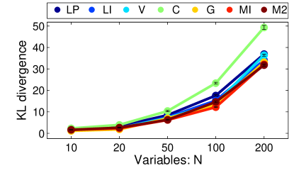
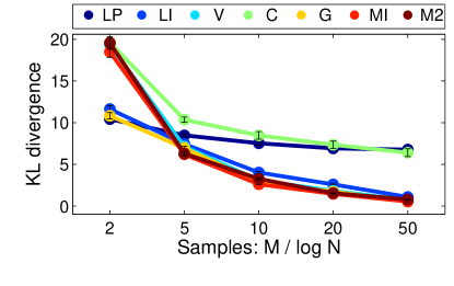
(a) , , overlap 1, density .05 (b) , , overlap 1, density .05
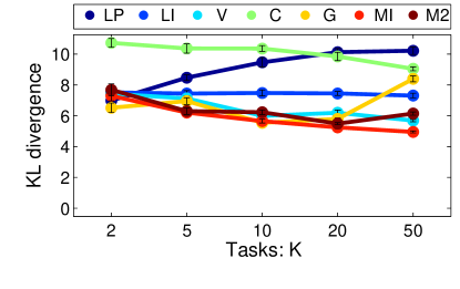
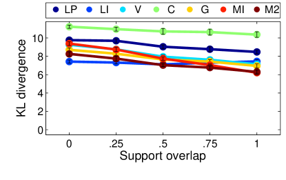
(c) , , overlap 1, density .05 (d) , , , density .05
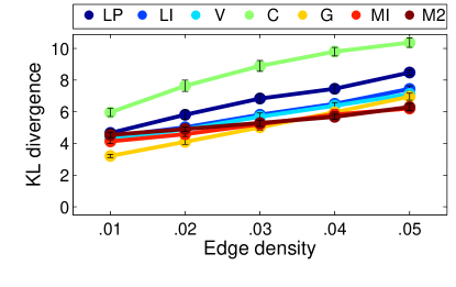
(e) , , , overlap 1
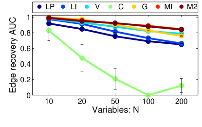
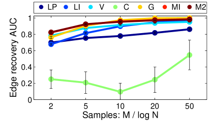
(a) , , overlap 1, density .05 (b) , , overlap 1, density .05
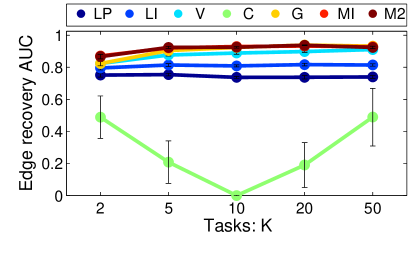
(c) , , overlap 1, density .05 (d) , , , density .05
(e) , , , overlap 1
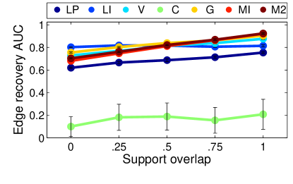
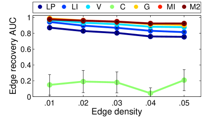
We begin with a synthetic example to test the ability of the method to recover the ground truth structure from data. The model contains variables and tasks. For each of repetitions, we perform the following steps. For each task , we generate a Gaussian graphical model with a required edge density (). The weight of each edge in is generated uniformly at random from . We ensure that the support overlap (i.e., the intersection of the edge sets across tasks) is equal to a prescribed proportion () of the support union. We guarantee positive definiteness of by verifying that its minimum eigenvalue is at least . We then generate samples for training and samples for validation, from each Gaussian graphical model . We use the validation set for selecting the optimal regularization parameter. Since all the tasks have the same number of samples, we set .
Figure 1 shows the Kullback-Leibler divergence between the models and the ground truth, for different number of variables, samples, tasks, support overlap between tasks, and edge density. The regularization parameter was selected in a validation set. Figure 2 shows the area under the curve of sensitivity vs. specificity of edge recovery for learnt models as the regularization level is varied, under the same scenarios as in Figure 1. Both our and multi-task methods produce better probability distributions (lower Kullback-Leibler divergence) than the comparison methods, except in the case of very small number of samples (), low support overlap between tasks (), or for low edge density (). Additionally, our multi-task methods recover the ground truth edges better (higher area under the curve) than the comparison methods, except in the case of low support overlap between tasks ().
6.2 Real-World Data Sets
| Site | Subjects | Scans | Site | Subjects | Scans | Site | Subjects | Scans |
|---|---|---|---|---|---|---|---|---|
| AnnArbor_a | 23 | 295 | Cleveland1 | 17 | 125 | NewYorkA2 | 24 | 192 |
| Baltimore | 46 | 120 | Cleveland2 | 14 | 125 | NewYorkB | 20 | 168 |
| Bangor | 20 | 256 | Dallas | 24 | 114 | Newark | 19 | 135 |
| Beijing1 | 40 | 225 | ICBM | 42 | 128 | Ontario | 11 | 100 |
| Beijing2 | 42 | 225 | Leiden1 | 12 | 210 | Orangeburg | 20 | 162 |
| Beijing3 | 41 | 225 | Leiden2 | 19 | 210 | Oulu1 | 57 | 243 |
| Beijing4 | 30 | 225 | Leipzig | 37 | 192 | Oulu2 | 47 | 243 |
| Beijing5 | 45 | 225 | NYU_TRT1A | 13 | 192 | Oxford | 22 | 175 |
| Berlin | 26 | 192 | NYU_TRT1B | 12 | 192 | PaloAlto | 17 | 234 |
| Cambridge1 | 48 | 117 | NYU_TRT2A | 13 | 192 | Queensland | 18 | 189 |
| Cambridge2 | 46 | 117 | NYU_TRT2B | 12 | 192 | SaintLouis | 31 | 125 |
| Cambridge3 | 49 | 117 | NYU_TRT3A | 13 | 192 | Taipei_a | 13 | 256 |
| Cambridge4 | 55 | 117 | NYU_TRT3B | 12 | 192 | Taipei_b | 8 | 160 |
| CambridgeWG | 35 | 144 | NewYorkA1 | 35 | 192 |
| Abbreviation | Cancer Type | Subjects |
|---|---|---|
| BRCA | Breast invasive carcinoma | 590 |
| COAD | Colon adenocarcinoma | 174 |
| GBM | Glioblastoma multiforme | 595 |
| LUSC | Lung squamous cell carcinoma | 155 |
| OV | Ovarian serous cystadenocarcinoma | 590 |
We chose two real-world data sets for experimental validation: the 1000 functional connectomes data set and the cancer genome atlas data set.
The 1000 functional connectomes data set contains resting-state fMRI of subjects collected on sites around the world. The data set is publicly available at http://www.nitrc.org/projects/fcon_1000/. Resting-state fMRI is a procedure that captures brain function of a subject that is at wakeful rest (i.e., not focused on the outside world). Registration of the data set to the same spatial reference template (Talairach space) and spatial smoothing was performed in SPM2 (http://www.fil.ion.ucl.ac.uk/spm/). We extracted voxels from the gray matter only, and grouped them into regions by using standard labels (See Appendix C.1), given by the Talairach Daemon (http://www.talairach.org/). These regions span the entire brain: cerebellum, cerebrum and brainstem. In order to capture laterality effects, we have regions for the left and right side of the brain. Table 2 shows the number of subjects per collection site as well as the number of scans per subject.
The cancer genome atlas data set contains gene expression data of subjects for various types of cancer. The data set is publicly available at http://tcga-data.nci.nih.gov/tcga/. We used genes commonly regulated in cancer (See Appendix C.2) that were identified on independent data sets by Lu et al. [2007]. Table 3 shows the number of subjects per collection site as well as the number of scans per subject.
(a) (b)
(c) (d)
(e) (f)
(a) (b)
(c) (d)
(e) (f)
(L)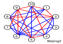
(V)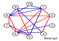
(C)
(G)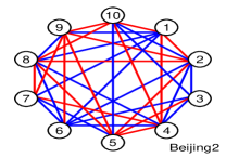
(MI)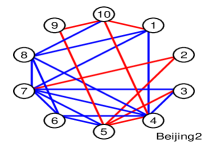
(M2)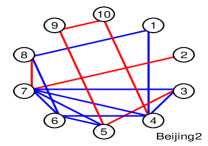
(L)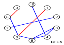
(V)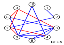
(C)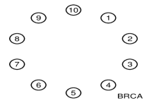
(G)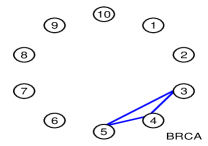
(MI)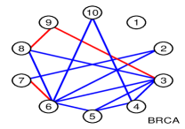
(M2)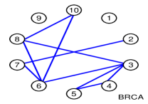
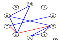
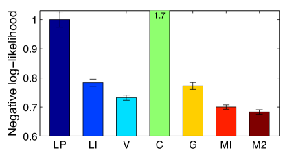
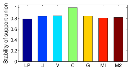
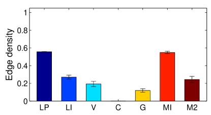
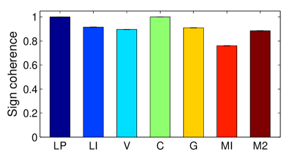
Our experimental setup is as follows. For the 1000 functional connectomes data set, we learn one Gaussian graphical model for each of the collection sites, i.e., each collection site is a task. For the cancer genome atlas data set, we learn one Gaussian graphical model for each of the five cancer types, i.e., each cancer type is a task. We used one third of the subjects for training, one third for validation and the remaining third for testing. We use the validation set for selecting the optimal regularization parameter, and the testing set for reporting log-likelihoods. We performed six repetitions by making each third of the subjects take turns as training, validation and testing sets.
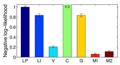
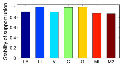
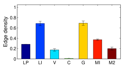
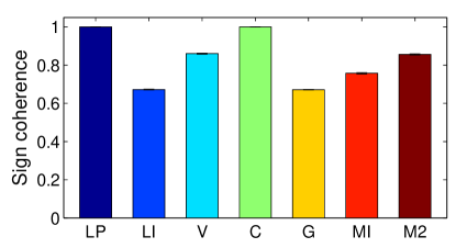
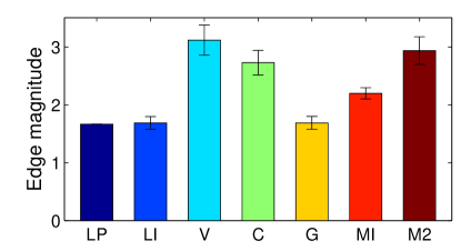
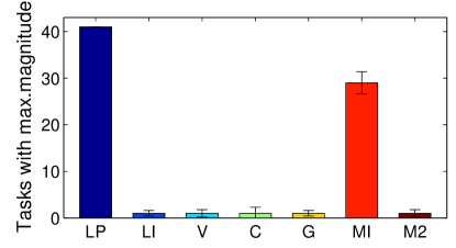
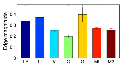
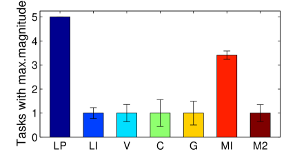
In Figures 3 and 4, we report the negative log-likelihood on the testing set, the stability of the support union across tasks, the edge density, the sign coherence across tasks, the average edge magnitude as well as the number of tasks where edges have maximum magnitude. The regularization parameter was selected in a validation set. For visualization purposes, we report the negative log-likelihood in the following fashion. After computing the negative log-likelihood, we subtracted the entropy measured on the testing set and then scaled the resulting value in . For computing our stability measure, we first computed the support union (i.e., the union of the edge sets across tasks) for each repetition. Then we averaged those adjacency matrices across repetitions and obtained a score for each node pair . We then transformed each score by setting since a node pair is stable when an edge is consistently present or absent. Finally, we averaged the transformed scores across all node pairs. For computing the sign coherence across tasks, we first computed for each node pair the proportion of tasks with positive sign as well as the proportion of tasks with negative sign . We then computed the score since a node pair is sign-coherent when an edge is consistently positive or negative. (Note that we exclude the case where the node pair is not an edge). Finally, we averaged the scores across all node pairs. The number of tasks where edges have maximum magnitude was first computed for each node pair , and then averaged across all node pairs. We can observe that the log-likelihood of both our and multi-task methods is better than the comparison methods. Both our and multi-task methods are relatively less stable than the comparison methods, due to the fact that the latter produce different topologies per task and thus, a bigger support union. Note that our multi-task method produces structures that are sparser than those produced by our counterpart. Additionally, edges in structures are more coherent in signs that those of structures. Furthermore, structures have approximately two thirds of the tasks have edges with maximum magnitude, while in structures only one task has an edge with maximum magnitude. In fact, Schmidt et al. [2011] noted that the -norm regularizer encourages values to have the same magnitude.
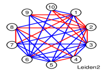
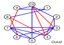
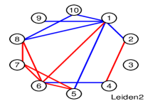
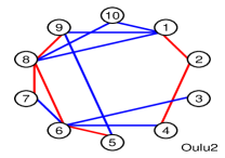
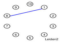
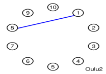
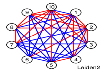
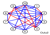
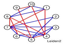
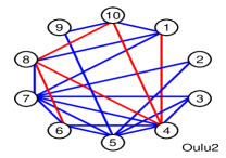
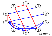
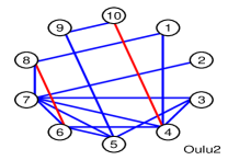
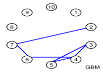
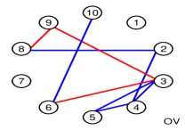
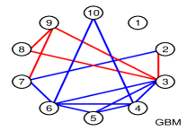
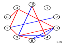
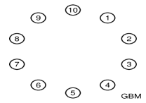
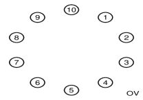
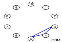
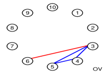
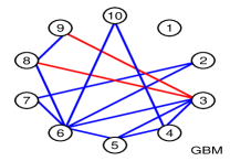
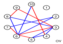
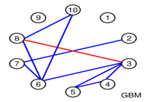
Figures 5 and 6 show a subgraph of learnt structures for three randomly selected tasks. The regularization parameter was selected in a validation set. We can observe that the sparsity pattern of the structures produced by our multi-task method is consistent across tasks. The comparison methods fail to obtain a consistent sparsity pattern. The exception is the method of Chiquet et al. [2011]. However, note in Figures 3(a) and 4(a) that the produced models do not generalize well on testing data.
Next, we identify and discuss edges that show the important differences between the tasks under analysis. We chose the edges are present in at least of the tasks, have sign coherence across tasks lower than , and have a partial correlation444The partial correlation is computed from the precision matrix in the same way that the correlation is computed from the covariance matrix. with a magnitude of at least .
In the 1000 functional connectomes data set, we identified only one edge between the Right Brodmann area 23 and the Left Brodmann area 30, by using our multi-task method. This edge is present in collection sites: sites had positive partial correlation (from to ), while sites had negative partial correlation (from to ). The Brodmann areas 23 and 30 have been identified as core regions associated with the default mode network which is active during wakeful rest [Buckner et al., 2008]. Thus, the fact that we find this edge across collection sites is clinically relevant. In comparison, our multi-task method found the edge in sites, the method of Guo et al. found the edge in sites, graphical lasso found the edge in sites, and the methods of Chiquet et al. and Varoquaux et al. did not find the edge in any collection site. In neuroscience, it is well known that the default mode network is disrupted with diseases such as autism spectrum disorders, schizophrenia and Alzheimer’s disease [Buckner et al., 2008]. We speculate that the difference in the collection sites ( with positive and with negative edge weights) could be explained by the presence of some subjects with an undetected disease. For instance, Broadmann areas 23 and 30 showed increased activity for depressed unmedicated patients in a resting-state positron emission tomography (PET) study [Monkul et al., 2012].
In the cancer genome atlas data set, we identified five edges which are present in all the cancer types, by using our multi-task method. In all of the cases, the edge weights were positive (or negative) in three cancer types and negative (or positive) in the remaining two cancer types. The edges are between the ABCA8 and PRC1 genes (partial correlation from to ), the ANP32E and CDC14B genes (partial correlation from to ), the FLJ20489 and TMEM4 genes (partial correlation from to ), the FMNL3 and FMO4 genes (partial correlation from to ) and the RPN2 and TMEPAI genes (partial correlation from to ). Two of these genes (FMNL3 and PRC1) have been previously linked to other types of cancer not analyzed here. The FMNL3 gene has been linked to pancreatic cancer [Jones et al., 2008]. The edge between the FMNL3 and FMO4 genes has the highest value for lung squamous cell carcinoma. Interestingly, lung cancer and pancreatic cancer are highly associated with tobacco use [Engeland et al., 1996]. Thus, the aforementioned genes (FMNL3 and FMO4) could be related to genetic predisposition. The PRC1 gene has been linked to melanoma [Pleasance et al., 2010]. The edge between the ABCA8 and PRC1 genes has the highest value for breast invasive carcinoma. Interestingly, women with breast cancer have a higher risk for melanoma and viceversa [Goggins et al., 2004].
7 Concluding Remarks
In this paper, we presented multi-task structure learning for Gaussian graphical models. We analyzed the sufficient number of samples for correctly recovering the support union and edge signs, for both sub-Gaussian random variables and variables with finite high-order moment. We also provide information-theoretic lower bounds. Our result implies that for sub-Gaussian variates, the polynomial-time method of regularization achieves optimal rates, since the necessary and the sufficient number of samples are both . Finally, we showed that multi-task learning is statistically more efficient than single-task learning, in the sense that multi-task learning requires less samples in order to avoid failure.
For experiments, we used a block coordinate descent method which is provably convergent and yields sparse and positive definite estimates. In synthetic experiments, we showed that the multi-task method outperforms others in recovering the topology of the ground truth model. Additionally, the cross-validated log-likelihood of the multi-task method is higher than the comparison methods in two real-world data sets.
There are several ways of extending this research. In this paper, we assume that the assignment of training samples to tasks is known. A more challenging setting comes from the assumption that the assignment of training samples to tasks is unknown. In this paper, we used the -norm regularizer. In the context of linear regression, it was shown that there are regimes in which the regularizer requires less samples than the regularizer, and viceversa [Negahban and Wainwright, 2011, Obozinski et al., 2011]. Dirty models have been shown superior to the previous two approaches [Jalali et al., 2010]. Thus, it is important to study the statistical efficiency of the methods such as [Hara and Washio, 2011, 2013]. Finally, in light of recent advances [Loh and Wainwright, 2013], it is also important to study the consistency of non-convex regularizers, such as [Guo et al., 2011, Zhu and Foygel, 2015].
Acknowledgments
We thank Dardo Tomasi for the preprocessing of the 1000 functional connectomes data set. This work was supported in part by NIDA Grants 1 R01 DA020949, 1 R01 DA023579 and NIBIB Grant 1 R01 EB007530.
Appendix A Detailed Proofs
In this section, we state the proofs of all the theorems in our manuscript.
A.1 Proof of Theorem 1
Here, we provide the detailed proof of Theorem 1. First, we derive some intermediate lemmas needed for the final proof.
Lemma 1.
Let . Let the -norm be the dual of the -norm, i.e., . Let be two vectors such that and . We have that, . Additionally, and , and therefore .
Proof.
From the identity for dual norms, we have . Let be the optimal solution for the previous maximization. That is, and . Thus, we obtained our assumptions.
First, we prove the statement by contradiction. Assume and . The objective function is linear and non-constant since , and the constraint set is convex. Thus, there is a unique optimal solution that must be on the boundary of the constraint set, i.e., . Therefore, we have a contradiction.
Next, we prove the statement and . Again, the objective function is linear and non-constant since , and the constraint set is convex. Thus, there is a unique optimal solution that must be on the boundary of the constraint set, i.e., . It is trivial to verify that for a vector that fulfills , we have that and . Therefore, the prescribed is indeed the unique optimal solution. Finally, for the prescribed , it is trivial to verify that . ∎
Lemma 2.
Let be two vectors such that and . We have that, . Let be the set of indices that attain the maximum value. Additionally, and for any set of weights such that , and therefore .
Proof.
From the identity for dual norms, we have . Let be the optimal solution for the previous maximization. That is, and . Thus, we obtained our assumptions.
We prove the first statement by contradiction. Assume and . The objective function is linear and non-constant since , and the constraint set is convex. Thus, there is a unique optimal solution that must be on the boundary of the constraint set, i.e., . Therefore, we have a contradiction.
The second statement can be found in Lemma 1 in [Negahban and Wainwright, 2011]. Note that by construction, the prescribed fulfills:
Finally, note that:
which proves our claim. ∎
Lemma 3.
Let and . Assume that and either or . If then . If then . If then .
Proof.
If , since we have .
If , since we have .
If , since we have . ∎
Lemma 4.
Let the -norm be the dual of the -norm, i.e., . Let Assumption A hold for the -norm and . Assume that . Set the regularization parameter in Eq. (3) to for some . If the following holds:
| (29) |
then we have:
Furthermore, the support union and the edge signs of the empirical minimizer are equal to those of the true model . That is:
provided that:
Proof.
Recall that the support union was formally defined in Eq. (6). For clarity, let the support union of the true model be . Let be the complement of . Additionally, we assume that every task contains the same number of samples, i.e., . Our proof makes use of some of the Karush-Kuhn-Tucker conditions, such as stationarity, complementary slackness, and dual feasibility. Given the length of the proof, we split it into four parts.
Part I. First, we show that the empirical minimizer correctly excludes all non-edges if it fulfills a strict dual feasibility condition. Note that the minimizer of the problem in Eq. (3) fulfills the stationarity condition. Let , we have:
| (30) |
where the -norm fulfills the dual feasibility condition:
| (31) |
For shortness, let and . By the complementary slackness condition, we have and thus:
| (32) |
By Eq. (31), Eq. (A.1) and Lemmas 1 and 2, for we have:
| (33) |
By Eq. (31), Eq. (A.1) and Lemma 1 for , we have:
| (34) |
By Eq. (31), Eq. (A.1) and Lemma 2 for , let be the set of indices that attain the maximum value, and be any set of weights such that . We have:
| (35) |
In particular, consider all edges . From Eq. (33), it follows that if the -norm fulfills a strict dual feasibility condition:
| (36) |
then , which implies that correctly excludes all non-edges, i.e., .
Part II. In what follows, we apply the primal-dual witness method. Our goal is to show that the strict dual feasibility condition is fulfilled.
To be clear, the following procedure is not a practical algorithm for solving Eq. (3). It is a proof technique for certifying the behavior of the empirical minimizer. We use in order to construct the primal-dual witness solution as follows:
-
a)
We determine in a manner that guarantees that and , by solving the restricted problem:
(37) - b)
-
c)
We set in order to guarantee that fulfills the stationarity condition in Eq. (30). That is:
(38) -
d)
We verify the strict dual feasibility condition. That is, by using Eq. (36), we verify that:
If the primal-dual witness construction succeeds, then it acts as a witness to the fact that the solution to the restricted problem in Eq. (37) is equal to the solution to the original (unrestricted) problem in Eq. (3). Note that all steps hold by construction, with the exception of step (d). Thus, in what follows, we concentrate on proving that step (d) holds under the assumptions made in this lemma.
First, note that by steps (a) and (c), the primal-dual witness solution fulfills the stationarity condition in Eq. (30). That is:
Let , and . By Eq. (5) we know that and thus:
| (39) |
Let be the vectorized form of matrix . By property of the Kronecker product and the definition in Eq. (8), we have:
Note that by step (a) we have . We then rewrite Eq. (39) as follows:
| (40.a) | |||
| (40.b) |
Since is invertible, from Eq. (40.a) we have:
By substituting in Eq. (40.b) and by defining as in Assumption A, we obtain:
| (41) |
Recall that . Given a set of vectors , define for shortness by independent products . Furthermore, define the -norm as follows:
| (42) |
where the last inequality follows from Assumption A. By using the -norm defined in Eq. (36) and the -norm defined in Eq. (42), it is easy to verify that:
| (43) |
Recall that we assumed that . Thus, the Eq. (A.1) becomes:
By assumption, we have that . For the moment, we will assume555In the next part of the proof, we show that this indeed holds. that . Since , we have . By Eq. (31), Eq. (42) and Eq. (A.1), we have:
Part III. Next, we show that the assumption in the previous part of the proof, indeed holds. Recall that . By Neumann series, we know that . Let , we have:
| (44) |
By replacing the above into the definition of , we have:
| (45) |
Define the norm . Note that where is defined in Eq. (9). Recall that by step (a) we have . Furthermore, by Eq. (7), each row/column in contains at most nonzero entries, thus . For the moment, we will assume that:
| (46) |
Given the above and by sub-multiplicativity of the -norm, we have:
and furthermore:
It is well known that as well as . By the above, sub-multiplicativity of the -norm and given that and as well as , we have from Eq. (A.1):
| (47) |
Thus, Eq. (A.1) provides an upper bound of for all . Recall that by step (a) we have . Define the function as follows , where:
| (48) |
Note that fulfills the stationarity condition in Eq. (30) if and only if is a fixed point of , that is . Define the ball:
| (49) |
Note that is continuous and that is convex and compact. By the Brouwer’s fixed point theorem [Ortega and Rheinboldt, 1970, p. 161], if maps into itself, then there exists some fixed point in . That is:
Note that by property of the Kronecker product and the definition in Eq. (8), we have:
Recall that and . By Eq. (A.1), Eq. (A.1) and the above observation, we can rewrite Eq. (48) as follows:
By assumption, we have that . Recall that we assumed that . By the above, Eq. (A.1) and since where is defined in Eq. (10), we have:
| (50) |
In order to finish the proof, we set in the ball defined in Eq. (49) so that Eq. (46), Eq. (A.1) and Eq. (A.1) are fulfilled with the proper constants. Recall that and thus . Assume that . Note that this implies that Eq. (49) is fulfilled and then . Our goal is to fulfill the conditions in Eq. (46), Eq. (A.1) and Eq. (A.1), that is:
| (51.a) | ||||
| (51.b) | ||||
| (51.c) |
As we will show, the above statements hold by using the following setting:
| (52) |
By Eq. (29) and Eq. (52), we have that Eq. (51.a) holds since:
| (53) |
By Eq. (29) and Eq. (52), we have that Eq. (51.b) holds since:
By Eq. (52) and Eq. (A.1), we have that Eq. (51.c) holds since:
Thus, we showed that .
Part IV. Here, we complete our proof. Since the primal-dual witness construction succeeded, the solution to the restricted problem in Eq. (37) is equal to the solution to the original (unrestricted) problem in Eq. (3). Recall that and thus . Since by Eq. (52) we have:
By our assumption that and by Lemma 3, it follows that the edge signs of are equal to those of . This together with the fact that implies that correctly recovers the support union, i.e., . ∎
Lemma 5.
Let . Assume that for each and , the random variable is zero-mean and sub-Gaussian with parameter . Assume that we are given i.i.d. samples for each of the tasks. For some , with probability at least , we have:
Proof.
Note that in order to bound , we need to simultaneously bound each entry of . We use Lemma 1 in [Ravikumar et al., 2011] since we assume that is zero-mean and sub-Gaussian with parameter . Thus, by using Lemma 1 in [Ravikumar et al., 2011] (for bounding each specific entry) and the union bound (for bounding simultaneously all entries for all tasks), we have for :
By solving for in the above, we get . By setting , we prove our claim. ∎
Next, we provide the final proof.
A.2 Proof of Theorem 2
Here, we provide the detailed proof of Theorem 2. First, we derive an intermediate lemma needed for the final proof. We also use Lemma 4 from the previous sub-section.
Lemma 6.
Let . Assume that for each and , the random variable is zero-mean and has -th moments upper bounded by . Assume that we are given i.i.d. samples for each of the tasks. For some , with probability at least , we have:
Proof.
Note that in order to bound , we need to simultaneously bound each entry of . We use Lemma 2 in [Ravikumar et al., 2011] since we assume that is zero-mean, and that there is a positive integer and a scalar such that . Thus, by using Lemma 2 in [Ravikumar et al., 2011] (for bounding each specific entry) and the union bound (for bounding simultaneously all entries for all tasks), we have:
By solving for in the above, we obtain . By setting , we prove our claim. ∎
Next, we provide the final proof.
A.3 Proof of Theorem 3
Here, we provide the detailed proof of Theorem 3. First, we derive an intermediate lemma needed for the final proof.
Lemma 7.
Assume are i.i.d. samples drawn from a bivariate Gaussian distribution with zero mean and identity covariance. The random variable follows a “Bessel” distribution with parameter , with density function:
where denotes the modified Bessel function of the second kind, and denotes the Gamma function. Furthermore:
where denotes the Meijer G-function and denotes the double factorial.
Proof.
Note that and are jointly independent and have density functions and respectively. By the product distribution formula, the density function of is given by . The characteristic function of is given by . The density function of the sum is given by . Note that as a function of can be defined as and therefore . By change of variables, the density function is the one stated in our claim.
The exact probability . The lower bound for can be obtained by using Taylor series. The upper bound for comes from the fact that the moment generating function of fulfills for . By Markov’s inequality and since are jointly independent, we have:
By optimally setting , we have . By the union bound, we have , and we prove that the stated upper bound holds. Note that we used the moment generating function upper bound for and thus . ∎
Next, we provide the final proof.
Proof of Theorem 3.
The proof is a specialization of Lemma 4 for a specific class of graphs. This will allow us obtain tighter results than the ones presented in Theorems 1 and 2. For clarity, let the support union of the true model be . Let be the complement of . Additionally, we assume that every task contains the same number of samples, i.e., . Given the length of the proof, we split it into four parts.
Part I. Here, we present our restricted model. Assume that is an even number and that we partition the set of nodes into pairs . That is, and for all . Let the true model have support:
| (54) |
Furthermore, assume that the algorithm knows that the diagonal elements in the true model are all equal to . With respect to our general analysis in Lemma 4, several things simplify in this restricted model. For each task , the true model is given by:
where for the node pair , we define:
Part II. Here, we show that a specifically constructed function governs the recovery of the true model. Let be the value of variable for sample and task . Let denote the data set formed by using only two variables and . Define the function as:
| (55) |
Note that by step (a) in the proof of Lemma 4, we have for all . Additionally, since we assume that , the stationarity condition in Eq. (38) is equivalent to:
Thus, by using Eq. (55), we have:
| (56) |
As we know, the above is related to the correct exclusion of all non-edges. Next, we focus on the correct inclusion of all edges. Recall that in our specific graph, the support is form by a partition of node pairs as in Eq. (54). Furthermore, since we assume that , the restricted problem in Eq. (37) reduces to solving for all node pairs :
Since we assume that the algorithm knows that the diagonal elements in the true model are all equal to , the above equation is equivalent to solving for every node pair :
The above problem has the minimizer if and only if belongs to the subdifferential set of the non-smooth objective function at . That is:
where is the dual variable satisfying the dual feasibility condition . Since the diagonal elements of are all equal to , we impose to guarantee positive definiteness. Thus, we can conclude that the optimal solution fulfills:
or equivalently by using Eq. (55), for all :
| (57) |
Thus, we obtained a simple expression for the correct inclusion of all edges.
Part III. Here, we analyze recovery success. The condition for correctly excluding all non-edges is that . By Eq. (56), this is equivalent to . The condition for correctly including all edges is given by Eq. (57). Putting both conditions together, our goal is to lower-bound the probability that:
Recall that . Assume that . By the union bound and Lemma 7, we have:
| (58) |
Next, we use Lemma 1 in [Ravikumar et al., 2011] since we assume that is zero-mean and sub-Gaussian with parameter . Recall that in our specific graph, the support is form by a partition of node pairs as in Eq. (54). Assume that . Assume that . By the union bound and Lemma 1 in [Ravikumar et al., 2011], we have:
| (59) |
In the above, without loss of generality, we assumed that , the proof is carried in the same way in the case that . For convenience, in order to obtain a simple expression, assume that . Thus, from Eq. (A.3) and Eq. (A.3), we have:
By solving for in the above, we get that recovery success is guaranteed with probability at least , provided that .
Part IV. Here, we analyze recovery failure by a proof by contradiction. Our goal is to show that if a solution exists with , then . This contradicts the dual feasibility condition in Eq. (31), and thus is not an optimal solution from the Karush-Kuhn-Tucker conditions. By Eq. (56), our goal is to lower-bound the probability that:
Next, we partition the set of nodes into pairs as follows. For , the pair contains one node from and one node from . The pair contains one node from and one node from . Note that by construction, if then and are independent for all . Define:
By Lemma 7 and since , we have:
By solving for in the above, we get that recovery failure is guaranteed with probability at least , provided that .
To complete the proof, we set . Note that we assume that . By positive definiteness, we have that . Furthermore, we assumed that and therefore . ∎
A.4 Proof of Theorem 4
Proof.
Assume we construct a block-diagonal matrix by arranging the precision matrices on its diagonal. Similarly, construct a matrix by arranging the precision matrices on its diagonal. Note that and since their blocks are positive definite as well. Furthermore, note that under this setting, each sample contains variables, and thus contains exactly samples in total. Our results follow from invoking Theorems 1 and 2 in [Wang et al., 2010] by using the samples and variables. ∎
A.5 Proof of Theorem 5
Proof.
If is a symmetric matrix, according to the Haynsworth inertia formula, if and only if its Schur complement and . By maximizing Eq. (22) with respect to , we get . This equality defines the optimal value for in Eq. (23). Since , the Schur complement is strictly positive.
Finally, in an iterative optimization algorithm, it suffices to initialize to a matrix that is known to be positive definite, e.g., a diagonal matrix with positive elements. ∎
A.6 Proof of Theorem 6
A.7 Proof of Theorem 7
Here, we provide the detailed proof of Theorem 7. First, we derive some intermediate lemmas needed for the final proof.
Lemma 8.
For , , , the regularized separable quadratic problem in Eq. (24) is equivalent to the separable quadratic problem with one constraint:
| (63) |
Furthermore, their optimal solutions are related by .
Proof.
Remark i.
In Eq. (63), we can assume that . If , the partial optimal solution is , and since this assignment does not affect the constraint, we can safely remove from the optimization problem.
Remark ii.
In what follows, we assume that . If , the unconstrained optimal solution of Eq. (63) is also its optimal solution, since is inside the feasible region given that .
Lemma 9.
For , , , the optimal solution of the separable quadratic problem with one constraint in Eq. (63) belongs to the same orthant as the unconstrained optimal solution , i.e., .
Proof.
We prove this by contradiction. Assume . Let be a vector such that and . The solution is feasible, since and . The difference in the objective function between and is:
Thus, the objective function for is smaller than for (the assumed optimal solution), which is a contradiction. ∎
Lemma 10.
For , , , the separable quadratic problem with one constraint in Eq. (63) is equivalent to the continuous quadratic knapsack problem:
| (64) |
Furthermore, their optimal solutions are related by .
Proof.
The continuous quadratic knapsack problem has been solved in several areas. Helgason et al. [1980] provides an algorithm which initially sort the breakpoints. Brucker [1984] and later Kiwiel [2007] provide deterministic linear-time algorithms by using medians of breakpoint subsets. In the context of machine learning, Duchi et al. [2008b] provides a randomized linear-time algorithm, while Liu et al. [2009a] provides an algorithm. We point out that Duchi et al. [2008b], Liu et al. [2009a] assume that the weights of the quadratic term are all equal, i.e., . Here, we assume arbitrary positive weights, i.e., .
Lemma 11.
For , , , the continuous quadratic knapsack problem in Eq. (64) has the solution:
| (65) |
for some , and furthermore, the optimal solution fulfills the condition:
Proof.
The Lagrangian of Eq. (64) is:
Both results can be obtained by invoking the Karush-Kuhn-Tucker optimality conditions on the above problem. ∎
Remark iii.
Lemma 12.
For , , , the continuous quadratic knapsack problem in Eq. (64) has the optimal solution for:
where the breakpoints are sorted in decreasing order by a permutation of the indices , i.e., .
Proof.
Given , can be found straightforwardly by using the equation of the line. In order to find , we search for the range in which:
which proves our claim. ∎
Next, we provide the final proof.
A.8 Proof of Theorem 8
Here, we provide the detailed proof of Theorem 8. First, we derive some intermediate lemmas needed for the final proof.
Lemma 13.
For , , , the regularized separable quadratic problem in Eq. (24) is equivalent to the separable quadratic trust-region problem:
| (66) |
Furthermore, their optimal solutions are related by .
Proof.
Remark iv.
In Eq. (66), we can assume that . If , the partial optimal solution is , and since this assignment does not affect the constraint, we can safely remove from the optimization problem.
Remark v.
In what follows, we assume that . If , the unconstrained optimal solution of Eq. (66) is also its optimal solution, since is inside the feasible region given that .
The trust-region problem has been extensively studied by the mathematical optimization community [Boyd and Vandenberghe, 2006, Forsythe and Golub, 1965, Moré and Sorensen, 1983]. Trust-region methods arise in the optimization of general convex functions. In that context, the strategy behind trust-region methods is to perform a local second-order approximation to the original objective function. The quadratic model for local optimization is “trusted” to be correct inside a circular region (i.e., the trust region). Separability is usually not assumed, i.e., a symmetric matrix is used instead of in Eq. (24), and therefore the general algorithms are more involved than ours. In the context of machine learning, Duchi and Singer [2009] provides a closed form solution for the separable version of the problem when the weights of the quadratic term are all equal, i.e., . In this paper, we assume arbitrary positive weights, i.e., . A closed form solution is not possible in this general case, but the efficient one-dimensional Newton-Raphson method can be applied.
Lemma 14.
For , , , the separable quadratic trust-region problem in Eq. (66) is equivalent to the problem:
| (67) |
Furthermore, their optimal solutions are related by .
Proof.
Remark vi.
Next, we provide the final proof.
Appendix B Algorithmic Details
First, we discuss the computational complexity the block coordinate descent method. Algorithm 1 has a time complexity of for iterations, variables and tasks. The polynomial dependence on the number of variables is expected since, in the general case, we cannot produce an algorithm faster than computing the inverse of the sample covariance in the case of an infinite sample. For , the linear-time dependence on the number of tasks can be accomplished by using a deterministic linear-time method by using medians of breakpoint subsets [Kiwiel, 2007]. A very easy-to-implement algorithm is obtained by initially sorting the breakpoints and searching the range for which Eq. (25) holds. For , the linear-time dependence on the number of tasks can be accomplished by using the one-dimensional Newton-Raphson method for solving Eq. (27). In our implementation, we initialize and perform 10 iterations of the Newton-Raphson method.
Next, we show that the block coordinate descent method converges to the optimal solution.
Lemma 15.
The solution sequence generated by the block coordinate descent method is bounded and every cluster point is a solution of the multi-task structure learning problem in Eq. (3).
Proof.
Finally, we show that we can reduce the size of the original problem by removing nodes that are not endpoints of any edge in the optimal solution. The rule for node removal depends only on the sample covariance matrix and thus, it can be applied as a preprocessing step.
Lemma 16.
Let the -norm be the dual of the -norm, i.e., . If the -norm fulfills , then the problem in Eq. (22) has the minimizer .
Appendix C Real-World Data Sets
In this section, we provide further details regarding the real-world data sets used in our experimental validation in Section 6.
C.1 1000 Functional Connectomes: Brain Regions
We present the list of the standard Talairach regions, from the 1000 functional connectomes data set. In order to abbreviate our presentation, we use parentheses, e.g., “(left, right) amygdala”, to indicate that we used two regions: left amygdala and right amygdala. The brain regions are the following:
-
•
Cerebellum: cerebellar lingual
-
•
Cerebellum: (culmen, declive, pyramis, tuber, uvula) of vermis
-
•
Cerebellum: (left, right) (cerebellar tonsil, culmen, declive, dentate, fastigium, inferior semi-lunar lobule, nodule, pyramis, tuber, uvula)
-
•
Cerebrum: hypothalamus
-
•
Cerebrum: (left, right) (amygdala, claustrum, hippocampus, pulvinar, putamen)
-
•
Cerebrum: (left, right) (anterior, lateral dorsal, lateral posterior, medial dorsal, midline, ventral anterior, ventral lateral, ventral posterior lateral, ventral posterior medial) nucleus
-
•
Cerebrum: (left, right) Brodmann area (1,2,…,47)
-
•
Cerebrum: (left, right) caudate (body, head, tail)
-
•
Cerebrum: (left, right) (lateral, medial) globus pallidus
-
•
Brainstem: (left, right) (mammillary body, red nucleus, substantia nigra, subthalamic nucleus)
C.2 The Cancer Genome Atlas: Genes
We present the list of the genes, from the cancer genome atlas data set. These genes are commonly regulated in cancer and were identified on independent data sets by Lu et al. [2007]. The genes are the following:
ABCA8, ABHD6, ACLY, ADAM10, ADAM12, ADHFE1, AGXT2, ALDH6A1, ANK2, ANKS1B, ANP32E, AP1S1, APOL2, ARL4D, ARPC1B, AURKA, AYTL2, BAT2D1, BAX, BFAR, BID, BOLA2, BRP44L, C10orf116, C17orf27, C1orf58, C1orf96, C5orf4, C6orf60, C8orf76, CALU, CARD4, CASC5, CBX3, CCNB2, CCT5, CDC14B, CDCA7, CEP55, CHRDL1, CIDEA, CKLF, CLEC3B, CLU, CNIH4, DBR1, DDX39, DHRS4, DKFZp667G2110, DKFZp762E1312, DMD, DNMT1, DTL, DTX3L, E2F3, ECHDC2, ECHDC3, EFCBP1, EFHC2, EIF2AK1, EIF2C2, EIF2S2, Ells1, EPHX2, EPRS, ERBB4, FAM107A, FAM49B, FARP1, FBXO3, FBXO32, FEN1, FEZ1, FKBP10, FKBP11, FLJ11286, FLJ14668, FLJ20489, FLJ20701, FLJ21511, FMNL3, FMO4, FNDC3B, FOXP1, FTL, GEMIN6, GLT25D1, GNL2, GOLPH2, GPR172A, GSTM5, GULP1, HDGF, HIF3A, HLA-F, HLF, HNRPK, HNRPU, HPSE2, HSPE1, ILF3, IPO9, IQGAP3, K-ALPHA-1, KCNAB1, KDELC1, KDELR2, KDELR3, KIAA1217, KIAA1715, LDHD, LOC162073, LOC91689, LRRFIP2, LSM4, MAGI1, MORC2, MPPE1, MSRA, MTERFD1, NAP1L1, NCL, NDRG2, NME1, NONO, NOX4, NPM1, NR3C2, NRP2, NUSAP1, P53AIP1, PALM, PAQR8, PDIA6, PGK1, PINK1, PLEKHB2, PLIN, PLOD3, PPAP2B, PPIH, PPP2R1B, PRC1, PSMA4, PSMA7, PSMB2, PSMB4, PSMB8, PTP4A3, RBAK, RECK, RORA, RPN2, SCNM1, SEMA6D, SFXN1, SHANK2, SLAMF8, SLC24A3, SLC38A1, SNCA, SNRPB, SNX10, SORBS2, SPP1, STAT1, SYNGR1, TAP1, TAPBP, TCEAL2, TMEM4, TMEPAI, TNFSF13B, TNPO1, TRPM3, TTK, TTL, TUBAL3, UBA2, USP2, UTP18, WASF3, WHSC1, WISP1, XTP3TPA, ZBTB12, ZWILCH.
References
- Banerjee et al. [2008] O. Banerjee, L. El Ghaoui, and A. d’Aspremont. Model Selection Through Sparse Maximum Likelihood Estimation for Multivariate Gaussian or Binary Data. Journal of Machine Learning Research, 9(Mar):485–516, 2008.
- Banerjee et al. [2006] O. Banerjee, L. El Ghaoui, A. d’Aspremont, and G. Natsoulis. Convex Optimization Techniques for Fitting Sparse Gaussian Graphical Models. International Conference on Machine Learning, pages 89–96, 2006.
- Boyd and Vandenberghe [2006] S. Boyd and L. Vandenberghe. Convex Optimization. Cambridge University Press, 2006.
- Brucker [1984] P. Brucker. An Algorithm for Quadratic Knapsack Problems. Operations Research Letters, 3(3):163–166, 1984.
- Buckner et al. [2008] R. Buckner, J. Andrews-Hanna, and D. Schacter. The Brain’s Default Network: Anatomy, Function, and Relevance to Disease. Annals of the New York Academy of Sciences, 1124:1–38, 2008.
- Cai et al. [2011] T. Cai, W. Liu, and X. Luo. A Constrained Minimization Approach to Sparse Precision Matrix Estimation. Journal of the American Statistical Association, 106(494):594–607, 2011.
- Chiquet et al. [2011] J. Chiquet, Y. Grandvalet, and C. Ambroise. Inferring Multiple Graphical Structures. Statistics and Computing, 21(4):537–553, 2011.
- Danaher et al. [2014] P. Danaher, P. Wang, and D. Witten. The Joint Graphical Lasso for Inverse Covariance Estimation Across Multiple Classes. Journal of the Royal Statistical Society: Series B, 76(2):373–397, 2014.
- d’Aspremont et al. [2008] A. d’Aspremont, O. Banerjee, and L. El Ghaoui. First-Order Methods for Sparse Covariance Selection. SIAM Journal on Matrix Analysis and Applications, 30(1):56–66, 2008.
- Dempster [1972] A. Dempster. Covariance Selection. Biometrics, 28(1):157–175, 1972.
- Dinh et al. [2013] Q. Dinh, A. Kyrillidis, and V. Cevher. A Proximal Newton Framework for Composite Minimization: Graph Learning without Cholesky Decompositions and Matrix Inversions. International Conference on Machine Learning, pages 271–279, 2013.
- Duchi et al. [2008a] J. Duchi, S. Gould, and D. Koller. Projected Subgradient Methods for Learning Sparse Gaussians. Uncertainty in Artificial Intelligence, pages 145–152, 2008a.
- Duchi et al. [2008b] J. Duchi, S. Shalev-Shwartz, Y. Singer, and T. Chandra. Efficient Projections onto the -Ball for Learning in High Dimensions. International Conference on Machine Learning, pages 272–279, 2008b.
- Duchi et al. [2010] J. Duchi, S. Shalev-Shwartz, Y. Singer, and A. Tewari. Composite Objective Mirror Descent. Conference on Learning Theory, pages 14–26, 2010.
- Duchi and Singer [2009] J. Duchi and Y. Singer. Efficient Learning using Forward-Backward Splitting. Neural Information Processing Systems, 22:495–503, 2009.
- Engeland et al. [1996] A. Engeland, A. Andersen, T. Haldorsen, and S. Tretli. Smoking Habits and Risk of Cancers Other than Lung Cancer: 28 years’ Follow-Up of 26,000 Norwegian Men and Women. Cancer Causes and Control, 7(5):497–506, 1996.
- Forsythe and Golub [1965] G. Forsythe and G. Golub. On the Stationary Values of a Second-Degree Polynomial on the Unit Sphere. SIAM Journal of the Society for Industrial and Applied Mathematics, 13(4):1050–1068, 1965.
- Friedman et al. [2007] J. Friedman, T. Hastie, and R. Tibshirani. Sparse Inverse Covariance Estimation with the Graphical Lasso. Biostatistics, 9(3):432–441, 2007.
- Goggins et al. [2004] W. Goggins, W. Gao, and H. Tsao. Association Between Female Breast Cancer and Cutaneous Melanoma. International Journal of Cancer, 111(5):792–794, 2004.
- Guillot et al. [2012] D. Guillot, B. Rajaratnam, B. Rolfs, A. Maleki, and I. Wong. Iterative Thresholding Algorithm for Sparse Inverse Covariance Estimation. Neural Information Processing Systems, 25:1574–1582, 2012.
- Guo et al. [2011] J. Guo, E. Levina, G. Michailidis, and J. Zhu. Joint Estimation of Multiple Graphical Models. Biometrika, 98(1):1–15, 2011.
- Hara and Washio [2011] S. Hara and T. Washio. Common Substructure Learning of Multiple Graphical Gaussian Models. European Conference on Machine Learning and Knowledge Discovery in Databases, 6912:1–16, 2011.
- Hara and Washio [2013] S. Hara and T. Washio. Learning a Common Substructure of Multiple Graphical Gaussian Models. Neural Networks, 38:23–38, 2013.
- Helgason et al. [1980] K. Helgason, J. Kennington, and H. Lall. A Polynomially Bounded Algorithm for a Singly Constrained Quadratic Program. Mathematical Programming, 18(1):338–343, 1980.
- Honorio et al. [2009] J. Honorio, L. Ortiz, D. Samaras, N. Paragios, and R. Goldstein. Sparse and Locally Constant Gaussian Graphical Models. Neural Information Processing Systems, 22:745–753, 2009.
- Honorio and Samaras [2010] J. Honorio and D. Samaras. Multi-Task Learning of Gaussian Graphical Models. International Conference on Machine Learning, pages 447–454, 2010.
- Honorio et al. [2012] J. Honorio, D. Samaras, I. Rish, and G. Cecchi. Variable Selection for Gaussian Graphical Models. International Conference on Artificial Intelligence and Statistics, 22:538–546, 2012.
- Hsieh et al. [2012] C. Hsieh, I. Dhillon, P. Ravikumar, and A. Banerjee. A Divide-and-Conquer Procedure for Sparse Inverse Covariance Estimation. Neural Information Processing Systems, 25:2330–2338, 2012.
- Hsieh et al. [2011] C. Hsieh, M. Sustik, I. Dhillon, and P. Ravikumar. Sparse Inverse Covariance Matrix Estimation Using Quadratic Approximation. Neural Information Processing Systems, 24:2330–2338, 2011.
- Hsieh et al. [2014] C. Hsieh, M. Sustik, I. Dhillon, and P. Ravikumar. QUIC: Quadratic Approximation for Sparse Inverse Covariance Estimation. Journal of Machine Learning Research, 15(Oct):2911–2947, 2014.
- Hsieh et al. [2013] C. Hsieh, M. Sustik, I. Dhillon, P. Ravikumar, and R. Poldrack. BIG & QUIC: Sparse Inverse Covariance Estimation for a Million Variables. Neural Information Processing Systems, 26:3165–3173, 2013.
- Jalali et al. [2010] A. Jalali, P. Ravikumar, S. Sanghavi, and C. Ruan. A Dirty Model for Multi-Task Learning. Neural Information Processing Systems, 23:964–972, 2010.
- Jebara [2004] T. Jebara. Multi-Task Feature and Kernel Selection for SVMs. International Conference on Machine Learning, pages 55–62, 2004.
- Johnson et al. [2012] C. Johnson, A. Jalali, and P. Ravikumar. High-Dimensional Sparse Inverse Covariance Estimation using Greedy Methods. International Conference on Artificial Intelligence and Statistics, 22:574–582, 2012.
- Jones et al. [2008] S. Jones, X. Zhang, D. Parsons, J. Lin, R. Leary, P. Angenendt, P. Mankoo, H. Carter, H. Kamiyama, A. Jimeno, S. Hong, B. Fu, M. Lin, E. Calhoun, M. Kamiyama, K. Walter, T. Nikolskaya, Y. Nikolsky, J. Hartigan, D. Smith, M. Hidalgo, S. Leach, A. Klein, E. Jaffee, M. Goggins, A. Maitra, C. Iacobuzio-Donahue, J. Eshleman, S. Kern, R. Hruban, R. Karchin, N. Papadopoulos, G. Parmigiani, B. Vogelstein, V. Velculescu, and K. Kinzler. Core Signaling Pathways in Human Pancreatic Cancers Revealed by Global Genomic Analyses. Science, 321(5897):1801–1806, 2008.
- Kambadur and Lozano [2013] P. Kambadur and A. Lozano. A Parallel, Block Greedy Method for Sparse Inverse Covariance Estimation for Ultra-high Dimensions. International Conference on Artificial Intelligence and Statistics, 23:351–359, 2013.
- Kiwiel [2007] K. Kiwiel. On Linear-Time Algorithms for the Continuous Quadratic Knapsack Problem. Journal of Optimization Theory and Applications, 134(3):549–554, 2007.
- Kolar et al. [2013] M. Kolar, H. Liu, and E. Xing. Markov Network Estimation from Multi-Attribute Data. International Conference on Machine Learning, pages 73–81, 2013.
- Kolar et al. [2014] M. Kolar, H. Liu, and E. Xing. Graph Estimation From Multi-Attribute Data. Journal of Machine Learning Research, 15(May):1713–1750, 2014.
- Kolar et al. [2009] M. Kolar, L. Song, and E. Xing. Sparsistent Learning of Varying-Coefficient Models with Structural Changes. Neural Information Processing Systems, 22:1006–1014, 2009.
- Lauritzen [1996] S. Lauritzen. Graphical Models. Oxford Press, 1996.
- Lee et al. [2006] S. Lee, V. Ganapathi, and D. Koller. Efficient Structure Learning of Markov Networks Using -Regularization. Neural Information Processing Systems, 19:817–824, 2006.
- Levina et al. [2008] E. Levina, A. Rothman, and J. Zhu. Sparse Estimation of Large Covariance Matrices via a Nested Lasso Penalty. The Annals of Applied Statistics, 2(1):245–263, 2008.
- Liu et al. [2009a] H. Liu, M. Palatucci, and J. Zhang. Blockwise Coordinate Descent Procedures for the Multi-task Lasso, with Applications to Neural Semantic Basis Discovery. International Conference on Machine Learning, pages 649–656, 2009a.
- Liu et al. [2009b] J. Liu, S. Ji, and J. Ye. Multi-Task Feature Learning Via Efficient -Norm Minimization. Uncertainty in Artificial Intelligence, pages 339–348, 2009b.
- Liu and Ihler [2011] Q. Liu and A. Ihler. Learning Scale Free Networks by Reweighted regularization. International Conference on Artificial Intelligence and Statistics, 15:40–48, 2011.
- Loh and Wainwright [2013] P. Loh and M. Wainwright. Regularized M-estimators with Nonconvexity: Statistical and Algorithmic Theory for Local Optima. Neural Information Processing Systems, 26:476–484, 2013.
- Lu et al. [2007] Y. Lu, Y. Yi, P. Liu, W. Wen, M. James, D. Wang, and M. You. Common Human Cancer Genes Discovered by Integrated Gene-Expression Analysis. Public Library of Science ONE, 2(11):e1149, 2007.
- Lu [2009] Z. Lu. Smooth Optimization Approach for Sparse Covariance Selection. SIAM Journal on Optimization, 19(4):1807–1827, 2009.
- Marlin and K.Murphy [2009] B. Marlin and K.Murphy. Sparse Gaussian Graphical Models with Unknown Block Structure. International Conference on Machine Learning, pages 705–712, 2009.
- Marlin et al. [2009] B. Marlin, M. Schmidt, and K. Murphy. Group Sparse Priors for Covariance Estimation. Uncertainty in Artificial Intelligence, pages 383–392, 2009.
- Meier et al. [2008] L. Meier, S. van de Geer, and P. Bühlmann. The Group Lasso for Logistic Regression. Journal of the Royal Statistical Society: Series B, 70(1):53–71, 2008.
- Meinshausen and Bühlmann [2006] N. Meinshausen and P. Bühlmann. High Dimensional Graphs and Variable Selection with the Lasso. The Annals of Statistics, 34(3):1436–1462, 2006.
- Mohan et al. [2012] K. Mohan, M. Chung, S. Han, D. Witten, S. Lee, and M. Fazel. Structured Learning of Gaussian Graphical Models. Neural Information Processing Systems, 25:620–628, 2012.
- Mohan et al. [2014] K. Mohan, P. London, M. Fazel, D. Witten, and S. Lee. Node-Based Learning of Multiple Gaussian Graphical Models. Journal of Machine Learning Research, 15(Feb):445–488, 2014.
- Monkul et al. [2012] E. Monkul, L. Silva, S. Narayana, M. Peluso, F. Zamarripa, F. Nery, P. Najt, J. Li, J. Lancaster, P. Fox, B. Lafer, and J. Soares. Abnormal Resting State Corticolimbic Blood Flow in Depressed Unmedicated Patients with Major Depression: A15O-H2O PET Study. Human Brain Mapping, 33(2):272–279, 2012.
- Moré and Sorensen [1983] J. Moré and D. Sorensen. Computing a Trust Region Step. SIAM Journal on Scientific and Statistical Computing, 4(3):553–572, 1983.
- Negahban and Wainwright [2011] S. Negahban and M. Wainwright. Simultaneous Support Recovery in High Dimensions: Benefits and Perils of Block -Regularization. IEEE Transactions on Information Theory, 57(6):3841–3863, 2011.
- Nemirovski et al. [2009] A. Nemirovski, A. Juditsky, G. Lan, and A. Shapiro. Robust Stochastic Approximation Approach to Stochastic Programming. SIAM Journal on Optimization, 19(4):1574–1609, 2009.
- Niculescu-Mizil and Caruana [2007] A. Niculescu-Mizil and R. Caruana. Inductive Transfer for Bayesian Network Structure Learning. International Conference on Artificial Intelligence and Statistics, 2:339–346, 2007.
- Obozinski et al. [2011] G. Obozinski, M. Wainwright, and M. Jordan. Support Union Recovery in High-Dimensional Multivariate Regression. The Annals of Statistics, 39(1):1–47, 2011.
- Olsen et al. [2012] P. Olsen, F. Oztoprak, J. Nocedal, and S. Rennie. Newton-Like Methods for Sparse Inverse Covariance Estimation. Neural Information Processing Systems, 25:755–763, 2012.
- Ortega and Rheinboldt [1970] J. Ortega and W. Rheinboldt. Iterative Solution of Nonlinear Equations in Several Variables. Academic Press, 1970.
- Oyen and Lane [2012] D. Oyen and T. Lane. Leveraging Domain Knowledge in Multitask Bayesian Network Structure Learning. AAAI Conference on Artificial Intelligence, pages 1091–1097, 2012.
- Peterson et al. [2015] C. Peterson, F. Stingo, and M. Vannucci. Bayesian Inference of Multiple Gaussian Graphical Models. Journal of the American Statistical Association, 110(509):159–174, 2015.
- Pleasance et al. [2010] E. Pleasance, R. Cheetham, P. Stephens, D. McBride, S. Humphray, C. Greenman, I. Varela, M. Lin, G. Ordóñez, G. Bignell, K. Ye, J. Alipaz, M. Bauer, D. Beare, A. Butler, R. Carter, L. Chen, A. Cox, S. Edkins, P. Kokko-Gonzales, N. Gormley, R. Grocock, C. Haudenschild, M. Hims, T. James, M. Jia, Z. Kingsbury, C. Leroy, J. Marshall, A. Menzies, L. Mudie, Z. Ning, T. Royce, O. Schulz-Trieglaff, A. Spiridou, L. Stebbings, L. Szajkowski, J. Teague, D. Williamson, L. Chin, M. Ross, P. Campbell, D. Bentley, P. Futreal, and M. Stratton. A Comprehensive Catalogue of Somatic Mutations from a Human Cancer Genome. Nature, 463:191–196, 2010.
- Qi et al. [2008] Y. Qi, D. Liu, L. Carin, and D. Dunson. Multi-Task Compressive Sensing with Dirichlet Process Priors. International Conference on Machine Learning, pages 768–775, 2008.
- Ravikumar et al. [2011] P. Ravikumar, M. Wainwright, G. Raskutti, and B. Yu. High-Dimensional Covariance Estimation by Minimizing -Penalized Log-Determinant Divergence. Electronic Journal of Statistics, 5:935–980, 2011.
- Rothman et al. [2008] A. Rothman, P. Bickel, E. Levina, and J. Zhu. Sparse Permutation Invariant Covariance Estimation. Electronic Journal of Statistics, 2:494–515, 2008.
- Scheinberg et al. [2010] K. Scheinberg, S. Ma, and D. Goldfarb. Sparse Inverse Covariance Selection via Alternating Linearization Methods. Neural Information Processing Systems, 23:2101–2109, 2010.
- Scheinberg and Rish [2010] K. Scheinberg and I. Rish. Learning Sparse Gaussian Markov Networks using a Greedy Coordinate Ascent Approach. European Conference on Machine Learning and Knowledge Discovery in Databases, 6323:196–212, 2010.
- Schmidt et al. [2011] M. Schmidt, N. Le Roux, and F. Bach. Convergence Rates of Inexact Proximal-Gradient Methods for Convex Optimization. Neural Information Processing Systems, 24:1458–1466, 2011.
- Schmidt et al. [2008] M. Schmidt, K. Murphy, G. Fung, and R. Rosales. Structure Learning in Random Fields for Heart Motion Abnormality Detection. IEEE Conference on Computer Vision and Pattern Recognition, pages 1–8, 2008.
- Schmidt et al. [2007] M. Schmidt, A. Niculescu-Mizil, and K. Murphy. Learning Graphical Model Structure Using -Regularization Paths. Association for the Advancement of Artificial Intelligence Conference, pages 1278–1283, 2007.
- Schmidt et al. [2009] M. Schmidt, E. van den Berg, M. Friedlander, and K. Murphy. Optimizing Costly Functions with Simple Constraints: A Limited-Memory Projected Quasi-Newton Algorithm. International Conference on Artificial Intelligence and Statistics, 5:456–463, 2009.
- Sun et al. [2013] S. Sun, Y. Zhu, and J. Xu. Adaptive Variable Clustering in Gaussian Graphical Models. International Conference on Artificial Intelligence and Statistics, 33:931–939, 2013.
- Treister and Turek [2014] E. Treister and J. Turek. A Block-Coordinate Descent Approach for Large-Scale Sparse Inverse Covariance Estimation. Neural Information Processing Systems, 27:927–935, 2014.
- Tropp [2006] J. Tropp. Algorithms for Simultaneous Sparse Approximation, Part II: Convex Relaxation. Signal Processing, 86(3):589–602, 2006.
- Tseng [2001] P. Tseng. Convergence of a Block Coordinate Descent Method for Nondifferentiable Minimization. Journal of Optimization Theory and Applications, 109(3):475–494, 2001.
- Turlach et al. [2005] B. Turlach, W. Venables, and S. Wright. Simultaneous Variable Selection. Technometrics, 47(3):349–363, 2005.
- Varoquaux et al. [2010] G. Varoquaux, A. Gramfort, J. Poline, and B. Thirion. Brain Covariance Selection: Better Individual Functional Connectivity Models Using Population Prior. Neural Information Processing Systems, 23:2334–2342, 2010.
- Wainwright [2009] M. Wainwright. Sharp Thresholds for High-Dimensional and Noisy Sparsity Recovery Using Constrained Quadratic Programming (Lasso). IEEE Transactions on Information Theory, 55(5):2183–2202, 2009.
- Wainwright et al. [2006] M. Wainwright, P. Ravikumar, and J. Lafferty. High-Dimensional Graphical Model Selection Using -Regularized Logistic Regression. Neural Information Processing Systems, 19:1465–1472, 2006.
- Wang et al. [2013] H. Wang, A. Banerjee, C. Hsieh, P. Ravikumar, and I. Dhillon. Large Scale Distributed Sparse Precision Estimation. Neural Information Processing Systems, 26:584–592, 2013.
- Wang et al. [2010] W. Wang, M. Wainwright, and K. Ramchandran. Information-Theoretic Bounds on Model Selection for Gaussian Markov Random Fields. IEEE International Symposium on Information Theory, pages 1373 – 1377, 2010.
- Wilson et al. [2007] A. Wilson, A. Fern, S. Ray, and P. Tadepalli. Multi-Task Reinforcement Learning: A Hierarchical Bayesian Approach. International Conference on Machine Learning, pages 1015–1022, 2007.
- Xiao [2010] L. Xiao. Dual Averaging Methods for Regularized Stochastic Learning and Online Optimization. Journal of Machine Learning Research, 11(Oct):2543–2596, 2010.
- Yang et al. [2013] J. Yang, D. Sun, and K. Toh. A Proximal Point Algorithm for Log-Determinant Optimization with Group Lasso Regularization. SIAM Journal on Optimization, 23(2):857–893, 2013.
- Yu et al. [2008] J. Yu, S. Vishwanathan, S. Günter, and N. Schraudolph. A Quasi-Newton Approach to Nonsmooth Convex Optimization. International Conference on Machine Learning, pages 1216–1223, 2008.
- Yuan [2010] M. Yuan. High Dimensional Inverse Covariance Matrix Estimation via Linear Programming. Journal of Machine Learning Research, 11(Aug):2261–2286, 2010.
- Yuan and Lin [2006] M. Yuan and Y. Lin. Model Selection and Estimation in Regression with Grouped Variables. Journal of the Royal Statistical Society: Series B, 68(1):49–67, 2006.
- Yuan and Lin [2007] M. Yuan and Y. Lin. Model Selection and Estimation in the Gaussian Graphical Model. Biometrika, 94(1):19–35, 2007.
- Yun et al. [2011] S. Yun, P. Tseng, and K. Toh. A Block Coordinate Gradient Descent Method for Regularized Convex Separable Optimization and Covariance Selection. Mathematical Programming, 129(2):331–355, 2011.
- Zhang and Wang [2010] B. Zhang and Y. Wang. Learning Structural Changes of Gaussian Graphical Models in Controlled Experiments. Uncertainty in Artificial Intelligence, pages 701–708, 2010.
- Zhou et al. [2011] S. Zhou, P. Rütimann, M. Xu, and P. Bühlmann. High-Dimensional Covariance Estimation Based On Gaussian Graphical Models. Journal of Machine Learning Research, 12(Oct):2975–3026, 2011.
- Zhu and Foygel [2015] Y. Zhu and R. Foygel. The Log-Shift Penalty for Adaptive Estimation of Multiple Gaussian Graphical Models. International Conference on Artificial Intelligence and Statistics, 38:1153–1161, 2015.