An analytical comparison of coalescent-based multilocus methods: The three-taxon case

Abstract

Incomplete lineage sorting (ILS) is a common source of gene tree incongruence in multilocus analyses. A large number of methods have been developed to infer species trees in the presence of ILS. Here we provide a mathematical analysis of several coalescent-based methods. Our analysis is performed on a three-taxon species tree and assumes that the gene trees are correctly reconstructed along with their branch lengths.

1 Introduction

Incomplete lineage sorting (ILS) is an important confounding factor in phylogenetic analyses based on multiple genes or loci [Mad97, DR09]. ILS is a population-level phenomenon that is caused by the failure of two lineages to coalesce in a population, leading to the possibility that one of the lineages first coalesces with a lineage from a less closely related population. As a result, it can produce extensive gene tree incongruence that must be accounted for appropriately in multilocus analyses [DR06].

A large number of methods have been developed to address this source of incongruence [LYK⁺09]. Several such methods rely on a statistical model of ILS known as the multispecies coalescent. In this model, populations are connected by a phylogeny. Independent coalescent processes are performed in each population and assembled to produce gene trees. Several methods have been shown to be statistically consistent under the multispecies coalescent, that is, they are guaranteed to return the correct species tree given enough loci.

The performance and accuracy of coalescent-based multilocus methods have been the subject of numerous simulation studies [LR11, LYPE09, YN10]. In this paper, we complement such studies with a detailed analytical comparison in a tractable test case, a three-taxon species tree. We analyze 7 methods: maximum likelihood (ML), GLASS/Maximum Tree (MT), $R^{*}$, STAR, minimizing deep coalescences (MDC), STEAC, and shallowest coalescences (SC). Under the assumption that gene trees are reconstructed without estimation error, we derive the exponential decay rate of the failure probability as the internal branch length of the species tree varies. The analysis, which relies on large-deviations theory, reveals that ML and GLASS/MT are more accurate in this setting than the other methods—especially in the regime where ILS is more common.

2 Materials and Methods

2.1 Multispecies coalescent: Three-taxon case

We first describe the statistical model under which our analysis is performed, the multispecies coalescent. We only discuss the three-taxon case. For more details, see [DR09] and references therein.

A weighted rooted tree is called ultrametric if each leaf is exactly at the same distance from the root. For a three-leaf ultrametric tree $G$ with leaves $a$, $b$, and $c$, we denote by $ab|c$ the topology where $a$ and $b$ are closer to each other than to $c$, and similarly for $ac|b$, $bc|a$. The topology of $G$ is denoted by $\mathcal{T}[G]$.

Let $S$ be an ultrametric species phylogeny with three taxa. We assume that all haploid populations in $S$ have population size $N$. We denote the current populations by $\mathrm{A}$, $\mathrm{B}$ and $\mathrm{C}$ (which we identify with the leaves of $S$) and we assume that $S$ has topology $\mathrm{A}\mathrm{B}|\mathrm{C}$. The ancestral populations are $\mathrm{AB}$ (corresponding to the immediate ancestor to populations $\mathrm{A}$ and $\mathrm{B}$) and $\mathrm{ABC}$ (corresponding to the ancestor of populations $\mathrm{A}$, $\mathrm{B}$ and $\mathrm{C}$). The corresponding divergence times (backwards in time from the present) are denoted by $\tau_{\mathrm{AB}}$ and $\tau_{\mathrm{ABC}}$ with the assumption $\tau_{\mathrm{AB}}\leq\tau_{\mathrm{ABC}}$. All times are given in units of $N$ generations. For a population $\mathrm{X}$, we let $\tau^{\mathrm{P}}_{\mathrm{X}}$ be the divergence time of the parent population of $\mathrm{X}$. Let $\mathbb{X}=\{\mathrm{A},\mathrm{B},\mathrm{C},\mathrm{AB},\mathrm{ABC}\}$ be the set of all populations in $S$.

We consider $L$ loci $\ell=1,\ldots,L$ and, for each locus, we sample one lineage from each population at time $0$. For locus $\ell$, we denote by $I^{(\ell)}_{\mathrm{X}}$ the number of lineages entering population $\mathrm{X}$ and by $O^{(\ell)}_{\mathrm{X}}$ the number of lineages exiting population $X$ (backwards in time), where necessarily $I^{(\ell)}_{\mathrm{X}}\geq O^{(\ell)}_{\mathrm{X}}$. Similarly, for $k=O^{(\ell)}_{\mathrm{X}}+1,\ldots,I^{(\ell)}_{\mathrm{X}}$, the time of the coalescent event bringing the number of lineages from $k$ to $k-1$ in population $\mathrm{X}$ and locus $\ell$ is $T^{(\ell,k)}_{\mathrm{X}}$. We denote by $G_{1},\ldots,G_{L}$ the corresponding ultrametric gene trees (including both topology and branch lengths).

Then, under the multispecies coalescent, assuming the loci are unlinked, the likelihood of the gene trees is given by

$$f(G_{1},\ldots,G_{L}|S) = \prod_{\ell=1}^{L}\exp\bigg{(}-\sum_{\mathrm{X}\in\mathbb{X}}\bigg{\{}\binom{O^{(\ell)}_{\mathrm{X}}}{2}\left(\tau^{\mathrm{P}}_{\mathrm{X}}-T^{(\ell,O^{(\ell)}_{\mathrm{X}}+1)}_{\mathrm{X}}\right)$$ (1)

$$\quad\quad\quad\quad\quad-\sum_{k=O^{(\ell)}_{\mathrm{X}}+1}^{I^{(\ell)}_{\mathrm{X}}}\binom{k}{2}\left(T^{(\ell,k+1)}_{\mathrm{X}}+T^{(\ell,k)}_{\mathrm{X}}\right)\bigg{\}}\bigg{)}$$

where we let $T^{(\ell,I^{(\ell)}_{\mathrm{X}}+1)}_{\mathrm{X}}=\tau_{\mathrm{X}}$ for convenience [RY03].

The parameter governing the extent of incomplete lineage sorting is the length of the internal branch of $S$

$$t=\tau_{\mathrm{ABC}}-\tau_{\mathrm{AB}}.$$

The probability that the lineages from $\mathrm{A}$ and $\mathrm{B}$ fail to coalesce in branch $\mathrm{AB}$, an event we denote by $\textsc{Fail}_{\ell}$ for locus $\ell$ (and its complement by $\textsc{Success}_{\ell}$), is

$$1-p=e^{-t}.$$

Note that, in that case, all three gene-tree topologies are equally likely. Of course, $1-p\to 1$ as $t\to 0$.

2.2 Multilocus methods

A basic goal of multilocus analyses is to reconstruct a species phylogeny (including possibly estimates of the divergence times) from a collection of gene trees. Here we assume that the data consists of $L$ gene trees $G_{1},\ldots,G_{L}$ corresponding to $L$ unlinked loci generated under the multispecies coalescent. We assume further that the gene trees are ultrametric and that their topology and branch lengths are estimated without error.

We consider several common multilocus methods. In our setting, several of these methods are in fact equivalent and we therefore group them below. Note further that we only consider statistically consistent methods, that is, methods that are guaranteed to converge on the right species phylogeny as the number of loci $L$ increases to $+\infty$ (at least, in the test case we described above). We briefly describe these methods. For more details, see e.g. [LYK⁺09] and references therein.

ML/GLASS/MT

Under the multispecies coalescent, maximum likelihood (ML) selects the topology and divergence times that maximizes the likelihood (1).

In the GLASS method [MR10], the species phylogeny is reconstructed from a distance matrix in which the entries are the minimum gene coalescence times across loci. The equivalent Maximum Tree (MT) method was introduced and studied in [LP07, ELP07, LYP10].

A key result in [LYP10] is that, in the constant-population case, the term inside the exponential in the likelihood (1) is monotonically decreasing in the divergence times. As a result, because GLASS and MT select the phylogeny with the largest possible divergence times, maximum likelihood is equivalent to GLASS and MT in this context. See [LYP10] for details.

$R^{*}$/STAR/MDC

In the $R^{*}$ consensus method [Bry03, DDBR09], for each three-taxon set (here, we only have one such set), we include the topology that appears in highest frequency among the loci and we reconstruct the most resolved phylogeny that is compatible with these three-taxon topologies.

In the STAR method [LYPE09], the species phylogeny is reconstructed from a distance matrix in which the entries are the average ranks of gene coalescence times across loci. Here the root has the highest rank and the rank decreases by one as one goes from the root to the leaves.

The minimizing deep coalescences (MDC) method [Mad97, TN09] selects the species phylogeny that requires the smallest number of “extra lineages,” that is, lineages that fail to coalesce in a branch of the species phylogeny.

On a three-taxon phylogeny, there is only three distinct rooted topologies. In each case, the most recent divergence is assigned rank $1$ in STAR and the other divergence is assigned rank $2$. Hence selecting the topology corresponding to the lowest average rank is equivalent to selecting the most common topology among all loci—which is what $R^{*}$ does. A similar argument shows that MDC also selects the $R^{*}$ consensus tree in our test case.

STEAC/SC

In the STEAC method [LYPE09], the species phylogeny is reconstructed from a distance matrix in which the entries are the average coalescence times across loci. The shallowest coalescences (SC) method is similar to STEAC in that it uses average coalescence times. The difference between the two methods is in how they deal with multiple alleles per population. Since we only consider the single-allele case, the two methods are equivalent here.

2.3 Large-deviations approach

As mentioned above, we consider estimation methods that are statistically consistent in the sense that they are guaranteed to converge on the correct species phylogeny as the number of loci $L$ increases to $+\infty$. To compare different methods, we derive the rate of exponential decay of the probability of failure. Let $S$ be a species phylogeny with internal branch length $t$ and assume that $G_{1},\ldots,G_{L}$ are unlinked gene trees generated under the multispecies coalescent. As $L\to+\infty$, large-deviations theory (see e.g. [Dur96]) gives a characterization of the (exponential) decay rate

$$\alpha_{\mathbb{M}}(t)=-\lim_{L\to+\infty}\frac{1}{L}\ln\mathbb{P}[\text{Method $\mathbb{M}$ fails given $L$ loci from $S$}].$$

That is, roughly

$$\mathbb{P}[\text{Method $\mathbb{M}$ fails given $L$ loci from $S$}]\approx e^{-L\alpha_{\mathbb{M}}(t)},$$

for large $L$. As the notation indicates, the key parameter that influences the decay rate is the length of the internal branch $t$ of the species phylogeny. In particular, we expect that $\alpha_{\mathbb{M}}(t)$ is increasing in $t$ as a larger $t$ makes the reconstruction problem easier.

To derive $\alpha_{\mathbb{M}}(t)$, we express the probability of failure as a large deviation event of the form

$$\mathbb{P}[\text{Method $\mathbb{M}$ fails given $L$ loci from $S$}]=\mathbb{P}\left[\sum_{\ell=1}^{L}Y_{\ell}>yL\right],$$

where $y$ is a constant and $\{Y_{\ell}\}_{\ell=1}^{L}$ are independent identically distributed random variables. The particular choice of random variables depends on the method, as we explain below. Let

$$\phi(s)=\mathbb{E}[e^{sY_{\ell}}],$$

be the moment-generating function of $Y_{\ell}$ (which does not depend on $\ell$ by assumption). Then the decay rate is given by

$$\alpha_{\mathbb{M}}(t)=ys_{*}-\ln\phi(s_{*}),$$ (2)

where $s_{*}>0$ is the solution (if it exists) to

$$\frac{\phi^{\prime}(s_{*})}{\phi(s_{*})}=y,$$

provided there is an $s>0$ such that $\phi(s)<+\infty$, $y>\mathbb{E}[Y_{\ell}]$ and $Y_{\ell}$ is not a point mass at $\mathbb{E}[Y_{\ell}]$. For more details on large-deviations theory, see e.g. [Dur96].

3 Results

3.1 A domination result

We first argue that, given perfectly reconstructed unlinked gene trees under the multispecies coalescent, ML/GLASS/MT always has a greater probability of success than $R^{*}$/STAR/MDC and STEAC/SC—or, in fact, any other method. Indeed note that the probability of success can be divided into two cases:

1. The case where $\textsc{Success}_{\ell}$ occurs for at least one locus $\ell$, an event of probability $(1-(1-p)^{L})$. In that case, ML/GLASS/MT necessarily succeeds whereas the other two methods succeed with probability $<1$.

2. The case where $\textsc{Fail}_{\ell}$ occurs for all loci $\ell$, an event of probability $(1-p)^{L}$. In that case, all methods succeed with probability $1/3$ by symmetry. For instance, for ML/GLASS/MT, any pair of populations is equally likely to lead to the smallest inter-species distance. A similar argument applies to the other two methods.

Hence, overall ML/GLASS/MT succeeds with greater probability.

3.2 Decay rates

We derive the decay rates for the methods above. The results are plotted in Figure 1. The asymptotic regimes are highlighted in Figures 2 and 3. All proofs can be found in the appendix.

ML/GLASS/MT

In this case, the decay rate can be derived directly without using (2). Following the derivation in [MR10] (see also [LYP10] for a similar argument), ML/GLASS/MT succeeds with probability

$$(1-(1-p)^{L})+\frac{1}{3}(1-p)^{L}.$$

Then we get the following:

Claim 1 (ML/GLASS/MT)

The decay rate of ML/GLASS/MT on $S$ is

$$\alpha_{\mathrm{ML}}(t) = t.$$

$R^{*}$/STAR/MDC

For a locus $\ell$, we let $Z^{(\ell)}_{\mathrm{AB}}$ be $1$ if $\textsc{Fail}_{\ell}$ occurs and $\mathcal{T}[G_{\ell}]=\mathrm{A}\mathrm{B}|\mathrm{C}$, and $0$ otherwise. We let

$$\mathcal{Z}_{\mathrm{AB}}=\sum_{\ell=1}^{L}Z^{(\ell)}_{\mathrm{AB}}.$$

Similarly, we define $Z^{(\ell)}_{\mathrm{AC}}$, $Z^{(\ell)}_{\mathrm{BC}}$, $\mathcal{Z}_{\mathrm{AC}}$ and $\mathcal{Z}_{\mathrm{BC}}$. Then $R^{*}$/STAR/MDC fails if

$$\mathcal{Z}_{\mathrm{AB}}+(L-\mathcal{Z}_{\mathrm{AC}}-\mathcal{Z}_{\mathrm{BC}}-\mathcal{Z}_{\mathrm{AB}})<\max\{\mathcal{Z}_{\mathrm{AC}},\mathcal{Z}_{\mathrm{BC}}\}.$$

It can be shown that

$$\alpha_{\mathrm{R^{*}}}(t) = -\lim_{L\to+\infty}\frac{1}{L}\ln\mathbb{P}[2\mathcal{Z}_{\mathrm{AC}}+\mathcal{Z}_{\mathrm{BC}}>L].$$

Then we get the following:

Claim 2 ($R^{*}$/STAR/MDC)

The decay rate of $R^{*}$/STAR/MDC on $S$ is

$$\alpha_{\mathrm{R^{*}}}(t) = -\ln\left(2\sqrt{\frac{1}{3}e^{-t}\left(1-\frac{2}{3}e^{-t}\right)}+\frac{1}{3}e^{-t}\right).$$

As $t\to 0$,

$$\alpha_{\mathrm{R^{*}}}(t)=\frac{3}{4}t^{2}+O(t^{3}),$$

and, as $t\to+\infty$,

$$\alpha_{\mathrm{R^{*}}}(t)\approx\frac{t}{2}-\frac{1}{2}\ln\frac{4}{3}.$$

STEAC/SC

For a locus $\ell$, we let $D^{(\ell)}_{\mathrm{AB}}$ be the time to the most recent common ancestor of $\mathrm{A}$ and $\mathrm{B}$ in $G_{\ell}$ (in units of $N$ generations). We let

$$\mathcal{D}_{\mathrm{AB}}=\sum_{\ell=1}^{L}D^{(\ell)}_{\mathrm{AB}}.$$

Similarly, we define $D^{(\ell)}_{\mathrm{AC}}$, $D^{(\ell)}_{\mathrm{BC}}$, $\mathcal{D}_{\mathrm{AC}}$ and $\mathcal{D}_{\mathrm{BC}}$. Then STEAC/SC fails if

$$\mathcal{D}_{\mathrm{AB}}>\min\{\mathcal{D}_{\mathrm{AC}},\mathcal{D}_{\mathrm{BC}}\}.$$

It can be shown that

$$\alpha_{\mathrm{STEAC}}(t) = \lim_{L\to+\infty}-\frac{1}{L}\ln\mathbb{P}[\mathcal{D}_{\mathrm{AB}}-\mathcal{D}_{\mathrm{AC}}>0].$$

Then we get the following:

Claim 3 (STEAC/SC)

The decay rate of STEAC/SC on $S$ is

$$\alpha_{\mathrm{STEAC}}(t) = -\ln\left(\frac{3e^{-s_{*}t}-s_{*}^{2}e^{-t}}{3(1-s_{*}^{2})}\right),$$

where $0<s_{*}<1$ is the unique solution to the fixed-point equation

$$s_{*}=\frac{1}{2}[6s_{*}-3t(1-s_{*}^{2})]e^{(1-s_{*})t}.$$

Further, as $t\to 0$,

$$\alpha_{\mathrm{STEAC}}(t)=\frac{3}{8}t^{2}+O(t^{3}),$$

and, as $t\to+\infty$,

$$\alpha_{\mathrm{STEAC}}(t)\approx t-\ln t-0.1656.$$

Figure 1: Decay rates.

Figure 2: Decay rates as $t\to 0$. The dotted lines indicate the respective predicted asymptotics.

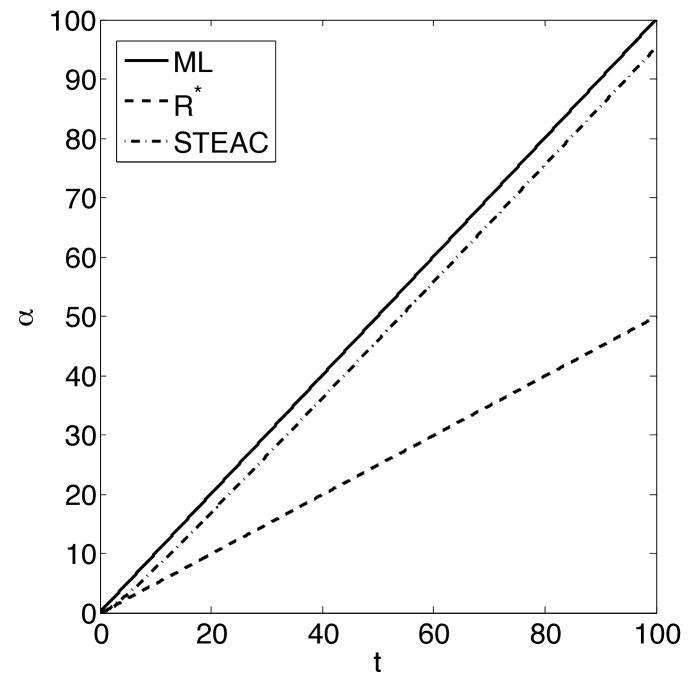
Figure 3: Decay rates as $t\to+\infty$.

4 Discussion

As can be seen from Figures 1, 2 and 3 as well as from the asymptotics, ML/GLASS/MT does indeed give a larger decay rate for all $t$. In fact, the decay rate of ML/GLASS/MT is significantly higher, especially as $t\to 0$ that is, under high levels of incomplete lineage sorting. For instance, to be concrete, if $L=500$ loci and $t=0.1$ (in units of $N$ generations), the probability of failure is approximately: $1.9\times 10^{-22}$ for ML/GLASS/MT; $0.038$ for $R^{*}$/STAR/MDC; $0.16$ for STEAC/SC. Intuitively, this difference in behavior arises from the fact that ML/GLASS/MT requires only one successful locus, whereas $R^{*}$/STAR/MDC and STEAC/SC rely on an average over all loci.

Comparing $R^{*}$/STAR/MDC and STEAC/SC, note that $\alpha_{\mathrm{R^{*}}}(t)$ is higher than $\alpha_{\mathrm{STEAC}}(t)$ for small $t$ but that the situation is reversed for large $t$. In fact, in the limit $t\to+\infty$, $\alpha_{\mathrm{STEAC}}(t)$ grows at roughly the same rate as the optimal $\alpha_{\mathrm{ML}}(t)$. At large $t$, STEAC/SC has somewhat of an advantage in that the expectation gap in the failure event increases linearly with $t$, whereas it saturates under $R^{*}$/STAR/MDC.

The analysis described here ignores several features that influence the accuracy of species tree reconstruction. Notably we have assumed that gene trees, including their branch lengths, are reconstructed without error. On real sequence datasets, the uncertainty arising from gene-tree estimation plays an important role. For instance, although GLASS/MT achieves the optimal decay rate in our setting, these methods are in fact sensitive to sequence noise because they rely on the computation of a minimum over loci—the very feature that leads to their superior performance here. Extending our analysis to incorporate gene tree estimation error is an important open problem which should help in the design of multilocus methods. It is important to note that, under appropriate modeling of sequence data, ML is not in general equivalent to GLASS/MT and is likely to be more robust to estimation error. In particular our analysis suggest that ML may be significantly more accurate than other methods in multilocus studies.

Other extensions deserve further study. Often many alleles are sampled from each population. Note that the benefit of multiple alleles is known to saturate as the number of alleles increases [Ros02]. This is because the probability of observing any number of alleles at the top of a branch is uniformly bounded in the number alleles existing at the bottom.

Further, the molecular clock assumption, although it may be a reasonable first approximation in the context of recently diverged populations, should not be necessary for our analysis. One should also consider larger numbers of taxa, varying population sizes, etc.

Simulation studies may provide further insight into these issues. However an analytical approach, such as the one we have used here, is valuable in that it allows the study of an entire class of models in one analysis. It can also provide useful, explicit predictions to guide the design of reconstruction procedures.

5 Acknowledgments

This work was supported by NSF grant DMS-1007144 and an Alfred P. Sloan Research Fellowship. Part of this work was performed while the author was visiting the Institute for Pure and Applied Mathematics (IPAM) at UCLA.

Appendix A Proofs

A.1 ML/GLASS/MT

Decay rate

Following the derivation in [MR10] (see also [LYP10] for a similar argument), ML/GLASS/MT succeeds with probability

$$(1-(1-p)^{L})+\frac{1}{3}(1-p)^{L},$$

where the two terms correspond to the two cases described in Section 3.1. Hence the decay rate of the failure probability is

$$\alpha_{\mathrm{ML}}(t) = \lim_{L\to+\infty}-\frac{1}{L}\ln\left\{1-(1-(1-p)^{L})+\frac{1}{3}(1-p)^{L}\right\}$$

$$= \lim_{L\to+\infty}-\frac{1}{L}\ln\left\{\frac{2}{3}(1-p)^{L}\right\}$$

$$= \lim_{L\to+\infty}\left\{-\frac{1}{L}\ln\frac{2}{3}-\ln(1-p)\right\}$$

$$= -\ln(1-p)$$

$$= t.$$

A.2 $R^{*}$/STAR/MDC

Definitions

For a locus $\ell$, we let $Z^{(\ell)}_{\mathrm{AB}}$ be $1$ if $\textsc{Fail}_{\ell}$ occurs and $\mathcal{T}[G_{\ell}]=\mathrm{A}\mathrm{B}|\mathrm{C}$, and $0$ otherwise. We let

$$\mathcal{Z}_{\mathrm{AB}}=\sum_{\ell=1}^{L}Z^{(\ell)}_{\mathrm{AB}}.$$

Similarly, we define $Z^{(\ell)}_{\mathrm{AC}}$, $Z^{(\ell)}_{\mathrm{BC}}$, $\mathcal{Z}_{\mathrm{AC}}$ and $\mathcal{Z}_{\mathrm{BC}}$. Then $R^{*}$/STAR/MDC fails if

$$\mathcal{Z}_{\mathrm{AB}}+(L-\mathcal{Z}_{\mathrm{AC}}-\mathcal{Z}_{\mathrm{BC}}-\mathcal{Z}_{\mathrm{AB}})<\max\{\mathcal{Z}_{\mathrm{AC}},\mathcal{Z}_{\mathrm{BC}}\},$$

an event we denote by $\mathcal{E}$. The second term on the LHS comes form the fact that, given $\textsc{Success}_{\ell}$, $\mathcal{T}[G_{\ell}]=\mathrm{A}\mathrm{B}|\mathrm{C}$. To deal with the term on the RHS, we re-write $\mathcal{E}$ as

$$2\max\{\mathcal{Z}_{\mathrm{AC}},\mathcal{Z}_{\mathrm{BC}}\}+\min\{\mathcal{Z}_{\mathrm{AC}},\mathcal{Z}_{\mathrm{BC}}\}>L,$$

and we use the auxiliary events

$$\mathcal{E}^{\prime}=\{2\mathcal{Z}_{\mathrm{AC}}+\mathcal{Z}_{\mathrm{BC}}>L\},$$

and

$$\mathcal{E}^{\prime\prime}=\{2\mathcal{Z}_{\mathrm{BC}}+\mathcal{Z}_{\mathrm{AC}}>L\},$$

to bound $\mathbb{P}[\mathcal{E}]$ as follows

$$\mathbb{P}[\mathcal{E}^{\prime}]\leq\mathbb{P}[\mathcal{E}]\leq\mathbb{P}[\mathcal{E}^{\prime}\cup\mathcal{E}^{\prime\prime}]\leq 2\mathbb{P}[\mathcal{E}^{\prime}],$$

where we used that $\mathbb{P}[\mathcal{E}^{\prime}]=\mathbb{P}[\mathcal{E}^{\prime\prime}]$ (by symmetry) in a union bound, and the fact that, on $\mathcal{E}^{\prime}$,

$$2\max\{\mathcal{Z}_{\mathrm{AC}},\mathcal{Z}_{\mathrm{BC}}\}+\min\{\mathcal{Z}_{\mathrm{AC}},\mathcal{Z}_{\mathrm{BC}}\}\geq 2\mathcal{Z}_{\mathrm{AC}}+\mathcal{Z}_{\mathrm{BC}}>L.$$

Hence

$$-\frac{1}{L}\ln\mathbb{P}[\mathcal{E}^{\prime}]\geq-\frac{1}{L}\ln\mathbb{P}[\mathcal{E}]\geq-\frac{1}{L}\ln 2\mathbb{P}[\mathcal{E}^{\prime}]=-\frac{1}{L}\ln\mathbb{P}[\mathcal{E}^{\prime}]-\frac{1}{L}\ln 2,$$

and, taking a limit as $L\to+\infty$,

$$\alpha_{\mathrm{R^{*}}}(t)=\lim_{L\to+\infty}-\frac{1}{L}\ln\mathbb{P}[\mathcal{E}]=\lim_{L\to+\infty}-\frac{1}{L}\ln\mathbb{P}[\mathcal{E}^{\prime}],$$

provided the limit exists.

Moment-generating function

In order to compute the limit above, we use the moment-generating function

$$\phi(s)=\mathbb{E}[\exp(s[2Z^{(\ell)}_{\mathrm{AC}}+Z^{(\ell)}_{\mathrm{BC}}])],$$

(which does not depend on $\ell$) as described in Section 2.3. Dividing up the expectation into the four possible cases, we have

$$\phi(s)=\left(p+\frac{1}{3}(1-p)\right)+\frac{1}{3}(1-p)(e^{s}+e^{2s})<+\infty,$$

for all $s\in\mathbb{R}$. Letting

$$W_{p}=\frac{1}{3}(1-p),$$

the derivative of $\phi(s)$ is

$$\phi^{\prime}(s)=W_{p}(e^{s}+2e^{2s}).$$

Decay rate

By large-deviations theory, we are looking for a solution to

$$1=\frac{\phi^{\prime}(s)}{\phi(s)}.$$

Letting $\omega=e^{s}$, we get the quadratic equation

$$\left(p+W_{p}\right)+W_{p}(\omega+\omega^{2})=W_{p}(\omega+2\omega^{2}),$$

or, rearranging,

$$\left(p+W_{p}\right)=W_{p}\omega^{2},$$

whose solution is

$$\omega_{*}=e^{s_{*}}=\sqrt{\frac{p+W_{p}}{W_{p}}}.$$

Then

$$\alpha_{\mathrm{R^{*}}}(t) = \lim_{L\to+\infty}-\frac{1}{L}\ln\mathbb{P}[\mathcal{E}^{\prime}]$$

$$= \lim_{L\to+\infty}-\frac{1}{L}\ln\mathbb{P}[2\mathcal{Z}_{\mathrm{AC}}+\mathcal{Z}_{\mathrm{BC}}>L]$$

$$= s_{*}-\ln\phi(s_{*}).$$

Noting that

$$\phi(s_{*}) = p+W_{p}+W_{p}\sqrt{\frac{p+W_{p}}{W_{p}}}+W_{p}\frac{p+W_{p}}{W_{p}}$$

$$= 2(p+W_{p})+\sqrt{(p+W_{p})W_{p}},$$

we get

$$s_{*}-\ln\phi(s_{*}) = \ln\left(\frac{\sqrt{p+W_{p}}}{2\sqrt{W_{p}}(p+W_{p})+W_{p}\sqrt{p+W_{p}}}\right),$$

Rearranging, we have finally

$$\alpha_{\mathrm{R^{*}}}(t) = -\ln\left(2\sqrt{W_{p}(p+W_{p})}+W_{p}\right)$$

$$= -\ln\left(2\sqrt{\frac{1}{3}e^{-t}\left(1-\frac{2}{3}e^{-t}\right)}+\frac{1}{3}e^{-t}\right).$$

Asymptotics

By a Taylor expansion, we get as $t\to 0$ that

$$\alpha_{\mathrm{R^{*}}}(t)=\frac{3}{4}t^{2}+O(t^{3}).$$

On the other hand, as $t\to+\infty$,

$$\alpha_{\mathrm{R^{*}}}(t) = -\ln\left(e^{-t/2}\left[2\sqrt{\frac{1}{3}\left(1-\frac{2}{3}e^{-t}\right)}+\frac{1}{3}e^{-t/2}\right]\right)$$

$$= \frac{t}{2}-\beta_{t}$$

where

$$\lim_{t\to+\infty}\beta_{t}=\frac{1}{2}\ln\frac{4}{3}.$$

A.3 STEAC/SC

Definitions

For a locus $\ell$, we let $D^{(\ell)}_{\mathrm{AB}}$ be the time to the most recent common ancestor of $\mathrm{A}$ and $\mathrm{B}$ in $G_{\ell}$ (in units of $N$ generations). We let

$$\mathcal{D}_{\mathrm{AB}}=\sum_{\ell=1}^{L}D^{(\ell)}_{\mathrm{AB}}.$$

Similarly, we define $D^{(\ell)}_{\mathrm{AC}}$, $D^{(\ell)}_{\mathrm{BC}}$, $\mathcal{D}_{\mathrm{AC}}$ and $\mathcal{D}_{\mathrm{BC}}$. Then STEAC/SC fails if

$$\mathcal{D}_{\mathrm{AB}}>\min\{\mathcal{D}_{\mathrm{AC}},\mathcal{D}_{\mathrm{BC}}\},$$

an event we denote by $\mathcal{E}$. Once again, to deal with the term on the RHS, we re-write $\mathcal{E}$ as

$$\mathcal{D}_{\mathrm{AB}}-\min\{\mathcal{D}_{\mathrm{AC}},\mathcal{D}_{\mathrm{BC}}\}>0,$$

and we use the auxiliary events

$$\mathcal{E}^{\prime}=\{\mathcal{D}_{\mathrm{AB}}-\mathcal{D}_{\mathrm{AC}}>0\},$$

and

$$\mathcal{E}^{\prime\prime}=\{\mathcal{D}_{\mathrm{AB}}-\mathcal{D}_{\mathrm{BC}}>0\},$$

to bound $\mathbb{P}[\mathcal{E}]$ as follows

$$\mathbb{P}[\mathcal{E}^{\prime}]\leq\mathbb{P}[\mathcal{E}]\leq\mathbb{P}[\mathcal{E}^{\prime}\cup\mathcal{E}^{\prime\prime}]\leq 2\mathbb{P}[\mathcal{E}^{\prime}],$$

where we used that $\mathbb{P}[\mathcal{E}^{\prime}]=\mathbb{P}[\mathcal{E}^{\prime\prime}]$ (by symmetry) in a union bound, and the fact that $\mathcal{E}^{\prime}$ implies $\mathcal{E}$. Hence

$$-\frac{1}{L}\ln\mathbb{P}[\mathcal{E}^{\prime}]\geq-\frac{1}{L}\ln\mathbb{P}[\mathcal{E}]\geq-\frac{1}{L}\ln 2\mathbb{P}[\mathcal{E}^{\prime}]=-\frac{1}{L}\ln\mathbb{P}[\mathcal{E}^{\prime}]-\frac{1}{L}\ln 2,$$

and, taking a limit as $L\to+\infty$,

$$\alpha_{\mathrm{STEAC}}(t)=\lim_{L\to+\infty}-\frac{1}{L}\ln\mathbb{P}[\mathcal{E}]=\lim_{L\to+\infty}-\frac{1}{L}\ln\mathbb{P}[\mathcal{E}^{\prime}],$$

provided the limit exists.

Moment-generating function

In order to compute the limit above, we need the moment-generating function

$$\phi(s)=\mathbb{E}[\exp(s[D^{(\ell)}_{\mathrm{AB}}-D^{(\ell)}_{\mathrm{AC}}])],$$

(which does not depend on $\ell$). Dividing up the expectation into the four possible cases, we have

$$\phi(s) = pe^{-st}\mathbb{E}\left[e^{s\tilde{E}_{0}}\right]\mathbb{E}\left[e^{-sE_{0}}\right]$$

$$+\frac{1}{3}(1-p)\mathbb{E}[e^{-sE_{1}}]$$

$$+\frac{1}{3}(1-p)\mathbb{E}[e^{sE_{1}}]$$

$$+\frac{1}{3}(1-p)$$

where we used:

1. In the case $\textsc{Success}_{\ell}$, $D^{(\ell)}_{\mathrm{AB}}-\tau_{\mathrm{AB}}=\tilde{E}_{0}$ where $\tilde{E}_{0}$ is an exponential mean $1$ conditioned to be less than $t$. Independently, using the memoryless property of the exponential, $D^{(\ell)}_{\mathrm{AC}}-\tau_{\mathrm{ABC}}=E_{0}$ where $E_{0}$ is an exponential mean $1$. Hence

   $$D^{(\ell)}_{\mathrm{AB}}-D^{(\ell)}_{\mathrm{AC}}=\tau_{\mathrm{AB}}+\tilde{E}_{0}-\tau_{\mathrm{ABC}}-E_{0}=-t+\tilde{E}_{0}-E_{0}.$$

2. In the case $\textsc{Fail}_{\ell}$ and $\mathcal{T}[G_{\ell}]=\mathrm{A}\mathrm{B}|\mathrm{C}$, $D^{(\ell)}_{\mathrm{AB}}-\tau_{\mathrm{ABC}}=\tilde{E}_{1}$ where $\tilde{E}_{1}$ the minimum of $\binom{3}{2}$ independent exponentials mean $1$, that is, an exponential mean $1/\binom{3}{2}=1/3$. Moreover, $D^{(\ell)}_{\mathrm{AC}}-\tau_{\mathrm{ABC}}=\tilde{E}_{1}+E_{1}$ where $E_{1}$ is an exponential mean $1$ independent of $\tilde{E}_{1}$. Hence

   $$D^{(\ell)}_{\mathrm{AB}}-D^{(\ell)}_{\mathrm{AC}}=\tau_{\mathrm{ABC}}+\tilde{E}_{1}-\tau_{\mathrm{ABC}}-\tilde{E}_{1}-E_{1}=-E_{1}.$$

3. In the case $\textsc{Fail}_{\ell}$ and $\mathcal{T}[G_{\ell}]=\mathrm{A}\mathrm{C}|\mathrm{B}$, $D^{(\ell)}_{\mathrm{AC}}-\tau_{\mathrm{ABC}}=\tilde{E}_{1}$ where $\tilde{E}_{1}$ is an exponential mean $1/\binom{3}{2}=1/3$. Moreover, $D^{(\ell)}_{\mathrm{AB}}-\tau_{\mathrm{ABC}}=\tilde{E}_{1}+E_{1}$ where $\mathbb{E}_{1}$ is an exponential mean $1$ independent of $\tilde{E}_{1}$.

   $$D^{(\ell)}_{\mathrm{AB}}-D^{(\ell)}_{\mathrm{AC}}=\tau_{\mathrm{ABC}}+\tilde{E}_{1}+E_{1}-\tau_{\mathrm{ABC}}-\tilde{E}_{1}=E_{1}.$$

4. In the case $\textsc{Fail}_{\ell}$ and $\mathcal{T}[G_{\ell}]=\mathrm{B}\mathrm{C}|\mathrm{A}$, $D^{(\ell)}_{\mathrm{AC}}=D^{(\ell)}_{\mathrm{AB}}$.

Note that

$$\mathbb{E}[e^{sE_{0}}]=\mathbb{E}[e^{sE_{1}}]=\frac{1}{1-s},$$

for all $|s|<1$, and

$$\mathbb{E}[e^{s\tilde{E}_{0}}]=\frac{1}{p}\int_{0}^{t}e^{sx}e^{-x}dx=\frac{1-e^{-(1-s)t}}{p(1-s)}.$$

Hence

$$\phi(s) = pe^{-st}\frac{1-e^{-(1-s)t}}{p(1-s)}\frac{1}{1+s}$$

$$+\frac{1}{3}(1-p)\left(\frac{1}{1+s}+\frac{1}{1-s}+1\right)$$

$$= \frac{e^{-st}-e^{-t}}{1-s^{2}}+\frac{1}{3}e^{-t}\left(\frac{3-s^{2}}{1-s^{2}}\right)$$

$$= \frac{3e^{-st}-s^{2}e^{-t}}{3(1-s^{2})}.$$

The derivative of $\phi(s)$ is

$$\phi^{\prime}(s) = \frac{[-3te^{-st}-2se^{-t}][3(1-s^{2})]-[3e^{-st}-s^{2}e^{-t}][-6s]}{[3(1-s^{2})]^{2}}$$

$$= \frac{[18s-9t(1-s^{2})]e^{-st}-6se^{-t}}{[3(1-s^{2})]^{2}}$$

Decay rate

By large-deviations theory, we are looking for a solution to

$$0=\frac{\phi^{\prime}(s)}{\phi(s)}=\frac{[6s-3t(1-s^{2})]e^{-st}-2se^{-t}}{(1-s^{2})(3e^{-st}-s^{2}e^{-t})}.$$ (3)

Note that the denominator on the RHS is positive on $s\in(0,1)$, and that

$$\frac{\phi^{\prime}(0)}{\phi(0)}=-t$$

and

$$\lim_{s\to 1^{-}}\frac{\phi^{\prime}(s)}{\phi(s)}=+\infty,$$

so that by [Dur96] there is a solution $0<s_{*}<1$ to (3). The solution $s_{*}$ must satisfy

$$[6s_{*}-3t(1-s_{*}^{2})]e^{-s_{*}t}-2s_{*}e^{-t}=0.$$ (4)

which can be re-written as the fixed-point equation

$$s_{*}=\frac{1}{2}[6s_{*}-3t(1-s_{*}^{2})]e^{(1-s_{*})t}\equiv F_{t}(s_{*}),\qquad 0<s_{*}<1.$$ (5)

Note that $F_{t}(0)=-3te^{t}\leq 0$ and $F_{t}(1)=3>1$. Moreover,

$$F_{t}^{\prime}(s) = \frac{1}{2}[6+6ts]e^{(1-s)t}-\frac{t}{2}[6s-3t(1-s^{2})]e^{(1-s)t}$$

$$= \frac{1}{2}e^{(1-s)t}[6+3t^{2}(1-s^{2})]>1,$$

for $0<s<1$. Hence $F_{t}(s)-s$ is strictly increasing and has a unique solution in $(0,1)$. Eq. (5) is easily solved numerically.

Then

$$\alpha_{\mathrm{STEAC}}(t) = \lim_{L\to+\infty}-\frac{1}{L}\ln\mathbb{P}[\mathcal{E}^{\prime}]$$

$$= \lim_{L\to+\infty}-\frac{1}{L}\ln\mathbb{P}[\mathcal{D}_{\mathrm{AB}}-\mathcal{D}_{\mathrm{AC}}>0]$$

$$= -\ln\phi(s_{*}).$$

Asymptotics

We consider asymptotics when $t\to 0$. Define

$$s_{\varepsilon}=\frac{3}{4}t+\varepsilon^{-1}t^{2}.$$

Evaluating the LHS in (4) (for $\varepsilon>0$ small but fixed) as $t\to 0$ gives

$$[6s_{\varepsilon}-3t(1-s_{\varepsilon}^{2})]e^{-s_{\varepsilon}t}-2s_{\varepsilon}e^{-t}$$

$$\quad=\left[\frac{9}{2}t+6\varepsilon^{-1}t^{2}-3t\left(1-\frac{9}{16}t^{2}+O(t^{3})\right)\right]\left[1-\frac{3}{4}t^{2}+O(t^{3})\right]$$

$$\quad\quad-\left[\frac{3}{2}t+2\varepsilon^{-1}t^{2}\right]\left[1-t+\frac{t^{2}}{2}+O(t^{3})\right]$$

$$\quad=\left[\frac{3}{2}t+6\varepsilon^{-1}t^{2}+O(t^{3})\right]\left[1-\frac{3}{4}t^{2}+O(t^{3})\right]$$

$$\quad\quad-\left[\frac{3}{2}t+2\varepsilon^{-1}t^{2}\right]\left[1-t+\frac{t^{2}}{2}+O(t^{3})\right]$$

$$\quad=\left[4\varepsilon^{-1}+\frac{3}{2}\right]t^{2}+O(t^{3}),$$

so that, because

$$4(-\varepsilon)^{-1}+\frac{3}{2}<0\quad\text{and}\quad 4\varepsilon^{-1}+\frac{3}{2}>0,$$

the solution of (4) satisfies $s_{-\varepsilon}<s_{*}<s_{\varepsilon}$ for $0<\varepsilon<\frac{8}{3}$ and $t$ small enough. Then

$$\phi(s_{\varepsilon}) = \frac{3e^{-s_{\varepsilon}t}-s_{\varepsilon}^{2}e^{-t}}{3(1-s_{\varepsilon}^{2})}$$

$$= \frac{1}{3}\left[3\left(1-\frac{3}{4}t^{2}+O(t^{3})\right)-\left(\frac{9}{16}t^{2}+O(t^{3})\right)\left(1-t+\frac{t^{2}}{2}+O(t^{3})\right)\right]$$

$$\quad\times\left[1+\frac{9}{16}t^{2}+O(t^{3})\right]$$

$$= 1+t^{2}\left\{-\frac{3}{4}-\frac{3}{16}+\frac{9}{16}\right\}+O(t^{3}).$$

Since this holds for all $\varepsilon>0$ small we get

$$\alpha_{\mathrm{STEAC}}(t)=-\ln\phi(s_{*})=\frac{3}{8}t^{2}+O(t^{3}).$$

For the $t\to+\infty$ asymptotics, let

$$u=\frac{1}{t}\quad\text{and}\quad\sigma=(1-s)t.$$

Substituting in (5), we get

$$1-\sigma u=\frac{1}{2}[6(1-\sigma u)-3\sigma(2-\sigma u)]e^{\sigma},$$

which after rearranging becomes

$$u = \frac{3e^{\sigma}-1-3\sigma e^{\sigma}}{3\sigma e^{\sigma}-\sigma-\frac{3}{2}\sigma^{2}e^{\sigma}}$$

$$= \frac{1}{\sigma(1+\frac{3\sigma e^{\sigma}}{2(3e^{\sigma}-1-3\sigma e^{\sigma})})}$$

$$\equiv \mathcal{F}(\sigma).$$

We have $\mathcal{F}(0)=+\infty$. Moreover, letting $\sigma_{*}$ be the only positive solution to

$$\mathcal{G}(\sigma_{*})\equiv 3e^{\sigma_{*}}-1-3\sigma_{*}e^{\sigma_{*}}=0,$$ (7)

we have $\mathcal{F}(\sigma_{*})=0$. Note that $\mathcal{G}^{\prime}(\sigma)=-3\sigma e^{\sigma}<0$, $\mathcal{G}(0)=2$ and $\lim_{\sigma\to+\infty}\mathcal{G}(\sigma)=-\infty$, so that $\sigma_{*}$ is well-defined. Noticing that $\mathcal{G}$ appears in the denominator of (A.3) as well we get that $\mathcal{F}$ is strictly decreasing between $\sigma=0$ and $\sigma=\sigma_{*}$. Hence the limit $t\to+\infty$ is equivalent to the limit $\sigma\to\sigma_{*}^{-}$. Finally, in that limit, letting $\sigma_{t}$ be the $\sigma$-value giving rise to the value $u=1/t$

$$\alpha_{\mathrm{STEAC}}(t) = -\ln\phi(s_{*})$$

$$= -\ln\frac{3e^{-s_{*}t}-s_{*}^{2}e^{-t}}{3(1-s_{*}^{2})}$$

$$= t-\ln\frac{3e^{\sigma_{t}}-(1-\frac{\sigma_{t}}{t})^{2}}{3(1-(1-\frac{\sigma_{t}}{t})^{2})}$$

$$= t-\ln\frac{3e^{\sigma_{t}}-1+\frac{2\sigma_{t}}{t}-\frac{\sigma_{t}^{2}}{t^{2}}}{3(\frac{2\sigma_{t}}{t}-\frac{\sigma_{t}^{2}}{t^{2}})}$$

$$= t-\ln t-\beta_{t},$$

where

$$\lim_{t\to+\infty}\beta_{t}=\ln\frac{3e^{\sigma_{*}}-1}{6\sigma_{*}}=\ln\frac{3\sigma_{*}e^{\sigma_{*}}}{6\sigma_{*}}=\sigma_{*}-\ln 2,$$

where we used (7).

References

• [Bry03] David Bryant. A classification of consensus methods for phylogenetics. In Bioconsensus (Piscataway, NJ, 2000/2001), volume 61 of DIMACS Ser. Discrete Math. Theoret. Comput. Sci., pages 163–183. Amer. Math. Soc., Providence, RI, 2003.
• [DDBR09] James H. Degnan, Michael DeGiorgio, David Bryant, and Noah A. Rosenberg. Properties of consensus methods for inferring species trees from gene trees. Systematic Biology, 58(1):35–54, 2009.
• [DR06] J. H. Degnan and N. A. Rosenberg. Discordance of species trees with their most likely gene trees. PLoS Genetics, 2(5), May 2006.
• [DR09] James H. Degnan and Noah A. Rosenberg. Gene tree discordance, phylogenetic inference and the multispecies coalescent. Trends in ecology and evolution, 24(6):332–340, 2009.
• [Dur96] Richard Durrett. Probability: theory and examples. Duxbury Press, Belmont, CA, second edition, 1996.
• [ELP07] Scott V. Edwards, Liang Liu, and Dennis K. Pearl. High-resolution species trees without concatenation. Proceedings of the National Academy of Sciences, 104(14):5936–5941, 2007.
• [LP07] Liang Liu and Dennis K. Pearl. Species trees from gene trees: Reconstructing bayesian posterior distributions of a species phylogeny using estimated gene tree distributions. Systematic Biology, 56(3):504–514, 2007.
• [LR11] Adam D. Leaché and Bruce Rannala. The accuracy of species tree estimation under simulation: A comparison of methods. Systematic Biology, 60(2):126–137, 2011.
• [LYK+09] Liang Liu, Lili Yu, Laura Kubatko, Dennis K. Pearl, and Scott V. Edwards. Coalescent methods for estimating phylogenetic trees. Molecular Phylogenetics and Evolution, 53(1):320 – 328, 2009.
• [LYP10] Liang Liu, Lili Yu, and Dennis Pearl. Maximum tree: a consistent estimator of the species tree. Journal of Mathematical Biology, 60:95–106, 2010. 10.1007/s00285-009-0260-0.
• [LYPE09] Liang Liu, Lili Yu, Dennis K. Pearl, and Scott V. Edwards. Estimating species phylogenies using coalescence times among sequences. Systematic Biology, 58(5):468–477, 2009.
• [Mad97] Wayne P. Maddison. Gene trees in species trees. Systematic Biology, 46(3):523–536, 1997.
• [MR10] Elchanan Mossel and Sébastien Roch. Incomplete lineage sorting: Consistent phylogeny estimation from multiple loci. IEEE/ACM Trans. Comput. Biology Bioinform., 7(1):166–171, 2010.
• [Roc12] Sebastien Roch. An analytical comparison of coalescent-based multilocus methods: The three-taxon case. Preprint, 2012.
• [Ros02] N. A. Rosenberg. The probability of topological concordance of gene trees and species trees. Theor. Popul. Biol., 61(2):225–247, March 2002.
• [RY03] Bruce Rannala and Ziheng Yang. Bayes estimation of species divergence times and ancestral population sizes using dna sequences from multiple loci. Genetics, 164(4):1645–1656, 2003.
• [TN09] Cuong Than and Luay Nakhleh. Species tree inference by minimizing deep coalescences. PLoS Comput Biol, 5(9):e1000501, 09 2009.
• [YN10] Yun Yu and Luay Nakhleh. The performance of methods for inferring species trees from multi-locus data. Preprint, 2010.