Pair correlation function for spin glasses

Abstract

We extract a pair correlation function (PCF) from probability distributions of the spin-overlap parameter $q$. The distributions come from Monte Carlo simulations. A measure, $w$, of the thermal fluctuations of magnetic patterns follows from the PCFs. We also obtain rms deviations (over different system samples) $\delta p$ away from average probabilities for $q$. For the linear system-sizes $L$ we have studied, (i) $w$ and $\delta p$ are independent of $L$ in the Edwards-Anderson model but scale as $1/L$ and $\sqrt{L}$, respectively, in the Sherrington-Kirkpatrik model.

Introduction—After decades of much work, the nature of the spin-glass (SG) phase is still unclear. A SG phase is found at low temperature in magnetic systems which are both quench-disordered and frustrated .libro ; s3 Random spin positions as well as random spin-spin couplings are sources of quenched disorder. When competition arises, because not all spin-spin coupling energies can be minimized simultaneously, a system is said to be frustrated. frustration Fixed disorder and built in competition are the two essential ingredients of complex systems.defc

The Sherrington-Kirkpatrick (SK) spin-glass model,SK in which each spin-spin coupling is assigned at random, without regard to spin-spin distance, is quench-disordered and frustrated. Its exact solution solution ; solution2 ; solution3 ; libro implies different random number seeds (which fully specify all couplings) can give rise, in thermal equilibrium, to magnetic patterns (MPs) which are macroscopically different. seedD Diversity of macroscopic observable magnitudes arising from random arrangements of microscopic constituents is the hallmark of complexity. complexity ; complexity1

However, no consensus has yet been reached on whether the macroscopic limit of the Edwards-AndersonEA (EA), in which only nearest-neighbor spins interact, (i) follows closely the SK model,opposite (ii) deviates from SK model behavior but nevertheless shows some diversity, halfway or (iii) fits a radically different picture, the droplet scenario, droplet ; bokil in which SGs with up-down symmetry can only be found in one of two macroscopic spin configurations which are related by global spin inversion. Thus, according to the droplet theory, the two necessary ingredients (quenched disorder and frustration) for complexity would become unable to generate diversity in the macroscopic limit of EA systems.

Complexity would make SGs rather exceptional among the many-particle systems of statistical physics. On the other hand, they would share this property with systems one finds elsewhere, such as in the life sciences, fraun information systems, is optimization problems, kirk and finance. finance In everyone of these fields complexity and diversity are the rule rather than the exception. Thus, addressing these issues in SGs with standard methods of statistical physics can lead to insight into other seemingly disconnected areas of research.

The basic tool for the characterization of the SG state is the spin overlap $q$ between two system states. libro To define it, let $\sigma_{i}^{(1)}$ be the spin of system state $1$ at site $i$, and similarly for $2$. Then, $q\equiv N^{-1}\Sigma_{i}\sigma_{i}^{(1)}\sigma_{i}^{(2)}$, i.e., $q$ is the average (over all sites) spin alignment between states $1$ and $2$. One usually lets states $1$ and $2$ be either (i) of a given time evolution of a given specimen at two widely different times, apart or (ii) of two independent ($1$ and $2$) time evolutions of the same specimen.

In macroscopic SK systems, the probability density (PD), $p(q)$, averaged over all realizations of quenched disorder (RQD), fulfills libro ; solution3 , (i) $p(q)\propto f(q)+\delta(q-q_{m})$ for $q\geq 0$, where $f(q)$ is a smooth function of $q$ for $q<q_{m}$ and $f(q)=0$ for $q\geq q_{m}$, and (ii) $p(q)=p(-q)$ if no magnetic field is applied (which we will assume throughout).

The fact that $f(q)\neq 0$ in the SK model implies the existence of ”odd” MPs (in addition to a pair of ordinary MPs that one expects to observe in all magnetic systems), whence complexity follows. Understandably, attempts at discerning between the macroscopic behaviors of the SK and EA models have focused on $p(q)$.

Specific system samples are interesting to examine. At least for finite-size EA systems, seed-dependent spin configurations do appear, much as in the SK model, asp , in thermal equilibrium. This is illustrated in Refs. [asp, ; pi, ], where plots of $p_{\cal J}(q)$ vs $q$ are shown for two different ${\cal J}$ sets of spin-spin couplings. Whereas some portions of $p_{\cal J}(q)$ differ drastically from sample to sample, the portions for larger values of $q$ are alike and all of them peak near $q=q_{m}$. We let self-overlap spikes (SOS) stand for spikes centered near $q_{m}$. Because they are all centered near the same position, the average of SOS (one for each RQD) over all RQD gives rise to the large peak at $q=q_{m}$. Spikes centered on smaller $q$ values, which vary randomly with different RQD, come from spin overlaps between states that belong to different basins of attraction. Accordingly, we refer to them as cross-overlap spikes (COS).

Interesting as it might be, statistical information on spike behavior has not, as far as we know, been available. Very little information on COS follows from the (average) behavior of $p(q)$. Cross-over spike statistics would enrich our picture of the SG state, somewhat as the pair correlation function does for the physics of liquids.

We aim to show how COS in $p_{\cal J}(q)$, of which the locations and shapes vary randomly over different RQD, can be added in a coherent fashion, in order to obtain a pair correlation function, $g(q\mid 0,Q)$, which is an average (in a sense which is defined below) over all RQD of all COS in the $0<q<Q$ range. We also (numerically) calculate the width of $g(q\mid 0,Q)$, which is a measure of MP thermal fluctuations, for $Q=1/2$. The results we obtain for low temperature ($T$) point to the following behavior: (i) $g(q\mid 0,1/2)$ closely follows a Lévy-flight like distribution, levy (ii) the pair correlation functions that follow from SOS and COS are roughly equal, that is $g(q\mid 0,1/2)\approx g(q\mid 1/2,1)$, (iii) the width of $g(q\mid 0,1/2)$ varies little, if at all, with linear system-size $L$ (scales as $1/L$) in the EA (SK) model. Thus, different ranges of spin-spin interaction give rise to qualitative differences between the complex behavior of spin glasses.

Models—We study the SK and EA models. In both of them, a $\sigma_{i}=\pm 1$ spin is located at each $i$-th site of a simple cubic lattice of $N=L^{3}$ sites. The interaction energy between a pair of spins at sites $i$ and $j$ is given by $J_{ij}\sigma_{i}\sigma_{j}$. We let $J_{ij}=\pm 1/\sqrt{N}$ randomly, without bias, for all $ij$ site pairs in the SK model. The transition temperature $T_{sg}$ between the paramagnetic and SG phase is $T_{sg}=1$. libro ; SK For the EA model, $J_{ij}=0$ unless $ij$ are nearest-neighbor pairs, and we draw each nearest-neighbor bond $J_{ij}$ independently from unbiased Gaussian distributions of unit variance. Then, $T_{sg}\simeq 0.95$. TcEA

We let $\langle u_{\cal J}\rangle_{\cal J}$ stand for the average of a thermal equilibrium quantity $u_{\cal J}$ over a number $N_{s}$ of different sets of random bonds $\{{\cal J}\}$.

Pair correlation function—Aiming for statistical information on COS at low temperature, we let

$$G_{\cal J}(q\mid Q_{1},Q_{2})=\int_{Q_{1}+h(-q)}^{Q_{2}-h(q)}dq_{1}\;p_{\cal J}(q_{1})p_{\cal J}(q_{1}+q),$$ (1)

where $h(q)=0$ if $q<0$ and $h(q)=q$ if $q\geq 0$. Clearly, $(\Delta Q-\mid q\mid)^{-1}G_{\cal J}(q\mid Q_{1},Q_{2})$, where $\Delta Q=Q_{2}-Q_{1}$, is the average of $p_{\cal J}(q_{1})p_{\cal J}(q_{1}+q)$ over the $({Q_{1}+h(-q)},{Q_{2}-h(q)})$ domain. We term ${G}(q\mid Q_{1},Q_{2})\equiv\langle{G}_{\cal J}(q\mid Q_{1},Q_{2})\rangle_{\cal J}$ pair correlation function.

The integral in Eq. (1) is as for the PD to be at $-q$ after a two-step random walk which starts at the origin, in which the length of both steps is identically distributed, but they are taken in opposite directions. Note that ${G}_{\cal J}(q\mid Q_{1},Q_{2})$ (i) peaks at $q=0$, fact (ii) is even with respect to $q=0$, since $p_{\cal J}(q)=p_{\cal J}(-q)$, and (iii) is somewhat broader than $p_{\cal J}(q)$ (from the theory of random walks).

The operation defined in Eq. (1) clearly displaces to $q=0$ any spike in $p_{\cal J}$ within the $(Q_{1},Q_{2})$ domain. Thus, by appropriate choice of $Q_{1}$ and $Q_{2}$ values, $G(q\mid Q_{1},Q_{2})$ enables one to make comparisons (see below) on equal footing of statistical information on SOS and COS.

We can also define $g(q\mid Q_{1},Q_{2})=BG(q\mid Q_{1},Q_{2})$, where $B\equiv 1/\int_{Q_{1}-Q_{2}}^{Q_{2}-Q_{1}}dq\;G(q\mid Q_{1},Q_{2})$. Note that $g(q\mid Q_{1},Q_{2})$ is the (conditional) PD that $q_{2}-q_{1}=q$, given that $q_{1},q_{2}\in(Q_{1},Q_{2})$. More specifically, assume all realizations of identical pairs of quenched disordered systems are evolving independently in equilibrium. Then, $g(q\mid Q_{1},Q_{2})$ is the PD for $q=q_{2}-q_{1}$, in the set of pairs of identical systems in which $q_{1},q_{2}\in(Q_{1},Q_{2})$ are observed at infinitely far apart times.

We define widths of two correlation functions. For a distribution function $F(x)$ such that $\int_{-\infty}^{\infty}dx\;xF(x)=0$, it makes sense to define a width $\delta x$ by $\delta xF(0)\equiv\int_{-\infty}^{\infty}dx\;F(x)$. Since $g(q\mid Q_{1},Q_{2})$ is normalized, we let

$$w(Q_{1},Q_{2})=1/g(0\mid Q_{1},Q_{2}).$$ (2)

For short, we let $w_{+}\equiv w(0,1/2)$, $w_{-}\equiv w(1/2,1)$. For $T\lesssim 0.3$, $w_{-}$ and $w_{+}$ are widths for COS and SOS, respectively. Furthermore, note (i) $g(q\mid Q_{1},Q_{2})\leq g(0\mid Q_{1},Q_{2})$ implies $w_{-},w_{+}\leq 1/2$, (ii) that we can think of $w_{-}$ as an intrinsic width of $g(q\mid 0,1/2)$, if $w_{-}\ll 1/2$, and similarly for $w_{+}$. We also define half-widths at half-maxima $\Gamma_{-}$ and $\Gamma_{+}$ by $2g(\Gamma_{-}\mid 0,1/2)=g(0\mid 0,1/2)$ and $2g(\Gamma_{+}\mid 1/2,1)=g(0\mid 1/2,1)$.

Table 1: The number of samples $N_{s}$ and the time $\tau_{s}$ taken for equilibration as well as for subsequent averaging is given in thousands of MC sweeps. Acceptance rates for system configuration exchanges at all $T$ are larger than or approximately equal to $A$. $\Delta T$ is the temperature spacing between systems in the tempered MC setup.

		SK				EA
L	4	6	8	4	6	8	10
$\tau_{s}$	$50$	$50$	$100$	$10$	$10^{2}$	$10^{3}$	$10^{4}$
$N_{s}$	$20$	$10$	$10$	$30$	$40$	$30$	$5$
$\Delta T$	$0.05$	$0.05$	$0.04$	$0.1$	$0.1$	$0.05$	$0.04$
$A$	$0.7$	$0.5$	$0.4$	$0.7$	$0.4$	$0.5$	$0.45$

Method—All numerical results given below follow from parallel tempered Monte Carlo (MC) simulations. tmc ; tmc3 ; paja We give all times in terms of MC sweeps.

All pairs of systems start running from independent random spin configurations. Each system pair is then allowed to come, in time $\tau_{s}$, to equilibrium with each reservoir of a string of them at $T$, $T+\Delta T$, $T+2\Delta T\;\ldots$, before readings of $q$ values are taken over an additional $\tau_{s}$ time span. From many such readings, the thermal equilibrium probability $p_{\cal J}(q)$, for a given RQD, is obtained for each temperature.

Relevant parameters for the simulations are in Table I.

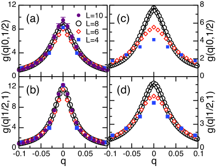
Figure 1: (a) Plots of $g(q\mid 0,1/2)$ vs $q$ for EA systems at $T=0.2$, with the values of $L$ shown. The full line is for a fit to the $L=8$ data points with $\Gamma^{\gamma}/[w(\Gamma^{\gamma}+\mid q\mid^{\gamma})]$. (b) Same as for (a) but for $g(q\mid 1/2,1)$. (c) Same as for (a) but for the SK model. (d) Same as for (a) but for $g(q\mid 1/2,1)$ for the SK model. Values of $w$ and $\Gamma$ are given in Fig. 2 for all $T$ and $L$ above, in both the EA and SK models. Values for $\gamma$ are given in the text.

Results for the pair correlation function—Data points for the pair correlation function are shown in Fig. 1 for $T=0.2$. The two graphs on the left hand side (right hand side) are for the EA (SK) model. The two top (bottom) graphs are for $Q_{1},Q_{2}=0,1/2$ ($Q_{1},Q_{2}=1/2,1$), which, since for $T\lesssim 0.3$, are for COS (SOS). While neither COS nor SOS exhibit significant size dependence in the EA model, they clearly do so in the SK model. We return to this point below.

All curves shown in Fig. 1 are rather pointed at the top. This is in contrast with the well known curves for $p(q)$ in the neighborhood of $q=q_{m}$ for finite SK systems pqm [but see Ref. asp, ; pi, for some $p_{\cal J}(q)$]. This is because values of $q_{m}$ vary over different RQD by amounts which, at least for $L=8$ and $T\lesssim 0.3$, are roughly equal to $\Gamma_{+}$ for the SK model. Thus, averaging $p_{\cal J}(q)$ over all RQD gives rise to a rounded $p(q)$ while $g(q\mid 1/2,1)$, being a coherent like superposition of spikes over different RQD, reveals their individual shapes.

Widths—We note that if $z=x_{1}+x_{2}$, and $x_{1}$ and $x_{2}$ are drawn from the above distribution, then, within a few per cent, in obvious notation, $\Gamma_{z}\simeq\Gamma_{x}2/\sqrt{\gamma-1}$ if $1.15\lesssim\gamma\leq 2$. Thus, $g(q\mid Q_{1},Q_{2})$ is approximately $2/\sqrt{\gamma-1}$ times wider than spikes in the $(Q_{1},Q_{2})$ domain.

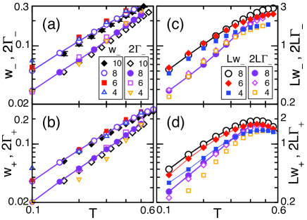
Figure 2: (a) Log-log plots of $w_{-}$ and $2\Gamma_{-}$ vs $T$, for EA systems of $L=4,6,8$ and $L=10$, as shown. Error bars for $L=10$ are shown, but for smaller $L$ values they are hidden by symbols. (b) Same as in (a) but for $w_{+}$ and $2\Gamma_{+}$. (c) Same as in (a) but for SK systems of $L=4,6$ and $L=8$, as shown. (d) Same as in (c) but for $Lw_{+}$ and $2L\Gamma_{+}$.

Good fits to all plots in Fig. 1 are provided by $\Gamma^{\gamma}/[w(\Gamma^{\gamma}+\mid q\mid^{\gamma})]$, which closely follows a Lévy flight distribution levy for $1<\gamma\leq 2$. Fits to the $L=8$ data are shown in Figs. 1(a), 1(b), 1(c) and 1(d). For both the EA and SK models, $\gamma\simeq 2(1-1/L)$ for all $T\lesssim 0.3$. Values for $w$ and $\Gamma$ are given in all panels of Fig. 2. As in Fig. 1, the two graphs on the left hand side (right hand side) are for the EA (SK) model. The two top (bottom) graphs are for $Q_{1},Q_{2}=0,1/2$ ($Q_{1},Q_{2}=1/2,1$), which for $T\lesssim 0.4$ are for COS (SOS).

Widths $w_{-}$ and $w_{+}$ appear in Figs. 2a and 2b to be size independent for $0<T\lesssim 0.3$. This points to finite widths for COS and SOS in the $L\rightarrow\infty$ limit of the EA model at low temperature. On the other hand, $w_{-},w_{+}\sim 1/L$ for large $L$ in the SK model seems consistent with the data points shown in Figs. 2c and 2d for $w_{-}$ and $w_{+}$. con

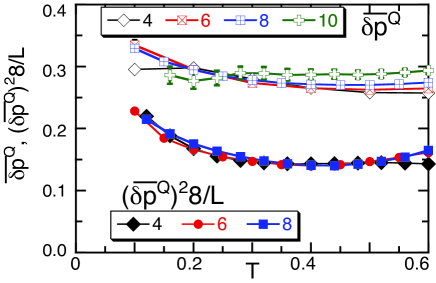
Figure 3: Plots of $(\overline{\delta p}^{Q})$ and of $(\overline{\delta p}^{Q})^{2}8/L$ vs $T$ for the EA and SK models, respectively, $Q=1/2$ and the values of $L$ shown. Except for $L=10$, icons cover all error bars.

Probability fluctuations over different RQD—Additional information follows from the (unnormalized) pair correlation function $G(q\mid Q_{1},Q_{2})$. For instance,

$$G(0\mid 0,Q)=Q[(\overline{p}^{Q})^{2}+(\overline{\delta p}^{Q})^{2}],$$ (3)

where $\overline{p}^{Q}$ and $(\overline{\delta p}^{Q})^{2}$ are the averages of ${p}$ and $(\delta p)^{2}$ over the $0<\mid q\mid<Q$ range, respectively.

Plots of $(\overline{\delta p}^{Q})$ vs $T$ for $Q=1/2$ and various systems sizes of the EA and SK models are shown in Fig. 3. Note that whereas $(\overline{\delta p}^{Q})$ scales as $\sim\sqrt{L}$ in the SK model, it appears to be, within statistical errors, independent of $L$ in the EA model.

The amount of fluctuations over different RQD of $X_{\cal J}(Q)$, defined by $X_{\cal J}(Q)=\int_{-Q}^{Q}dq\;p_{\cal J}(q)$, differs qualitatively from $(\overline{\delta p}^{Q})^{2}$ if $Q$ is not too small. This is because, $\langle X^{2}_{\cal J}(Q)\rangle_{\cal J}=w(0,Q)G(0\mid 0,Q)$, as follows from Eq. (2). Therefore, our result that $w(0,Q)(\overline{\delta p}^{Q})^{2}$ is independent of $L$ in both the EA and SK models if $Q\gg w(0,Q)$ implies $\langle X^{2}_{\cal J}(Q)\rangle_{\cal J}$ remains then bounded in both models as $L\rightarrow\infty$.

Conclusions—We have given a recipe for a coherent addition of self- and cross-overlap spikes (SOS and COS). The latter are centered on positions that vary randomly with RQD. In both the EA and SK models, the correlation functions for SOS and COS turn out to be approximately equal. The widths $w_{-}$ and $\Gamma_{-}$ (both for COS) give a measure of the thermal fluctuations of magnetic patterns. They are not too different from $w_{+}$ and $\Gamma_{+}$ (both for SOS), respectively. Neither $w_{\pm}$ nor $\Gamma_{\pm}$ vary much with linear system-size $L$ in the EA model but scale approximately as $1/L$ in the SK model. Their variation with system size at low temperature suggests they vanish in the macroscopic limit of the SK model but remain finite in the EA model. Finally, the mean square deviations of $p_{\cal J}$ away from $p(q)$ appear not to vary much with $L$ in the EA model but scale approximately as $L$ in the SK model.

The rule we have uncovered –which relates thermal fluctuations of magnetic patterns as well as probability fluctuations to interaction range– may well be valid in some broader domain, beyond the SK and EA models. For one, preliminary (unpublished) work yields similar results for some spatially disordered systems which are geometrically frustrated. Extensions to other fields of complex systems easily come to mind.

- (1) M. Mézard, G. Parisi, and M. Virasoro, Spin Glass Theory and Beyond (World Scientific, Singapore, 2004).
- (2) G. Aeppli and P. Chandra, Science 275, 177 (1997).
- (3) The importance of frustration in SGs was first brought out in, G. Toulouse, Commun. Math. Phys. 2, 115 (1977).
- (4) S. E. Page, Diversity and Complexity (Princeton University Press, Princeton, 2010); for a wide variety of definitions of complexity, see, S. Lloyd, IEEE Cntr. Syst. Mag. 21, 7 (2001).
- (5) D. Sherrington and S. Kirkpatrick, Phys. Rev. Lett. 32, 1792 (1975).
- (6) J. Thouless, P. W. Anderson, and R. Palmer, Philos. Mag. 35, 593 (1977).
- (7) A. J. Bray and M. A. Moore, Phys. Rev. Lett. 41, 1068 (1978).
- (8) G. Parisi, Phys. Rev. Lett. 43, 1754 (1979).
- (9) This was first shown to follow for the SK model in M. Mézard, G. Parisi, N. Sourlas, G. Toulouse, and M. Virasoro, Phys. Rev. Lett. 52, 1156 (1984).
- (10) This outlook follows after Parisi’s view of complexity in Biology, arXiv:cond-mat/9412018v1 (1994).
- (11) For a quantitative definition of complexity in spin glasses, as well as further references, see, for instance, T. Aspelmeier, A. J. Bray, and M. A. Moore, Phys. Rev. Lett. 92, 087203 (2004).
- (12) S. F. Edwards and P. W. Anderson, J. Phys. F 5, 965 (1975).
- (13) P. Contucci, C. Giardinà, C. Giberti, G. Parisi, and C. Vernia, Phys. Rev. Lett. 99, 057206 (2007); G. Parisi and F. Ricci-Tersenghi, Philos. Mag. 92, 341 (2012).
- (14) F. Krza̧kala and O. C. Martin, Phys. Rev. Lett. 85, 3013 (2000); M. Palassini and A. P. Young, Phys. Rev. Lett. 85, 3017 (2000); J. Houdayer and O. C. Martin, Europhys. Lett. 49, 794 (2000); M. Palassini, F. Liers, M. Juenger, and A. P. Young, Phys. Rev. B 68, 064413 (2003); G. Hed, A. P. Young, and E. Domany, Phys. Rev. Lett. 92, 157201 (2004).
- (15) D. S. Fisher and D. A. Huse, Phys. Rev. B 38, 386 (1988); M. A. Moore and A. J. Bray, J. Phys. C 18, L699 (1985); M. A. Moore, J. Phys A 38, L783 (2006).
- (16) H. Bokil, B. Drossel, and M. A. Moore, Phys. Rev. B 62, 946 (2000).
- (17) H. Fraunfelder, S. G. Sligar, P. G. Wolynes, Science 254, 1598 (1991).
- (18) See, for instance, M. Garey and D. S. Johnson, Computers and Intractability: A Guide to the Theory of NP-completeness (Freeman, San Francisco, 1979); N. Sourlas, Nature 339, 693 (1989); Y. Fu and P. W. Anderson, J. Phys. A 19 1605 (1986); For management information systems, see, for instance, The Oxford handbook of management information systems, edited by R. D. Galliers and W. L. Currie (Oxford University Press, Oxford, 2011).
- (19) S. Kirkpatrick, C. D. Gelatt, and M. P. Vecchi, Science 220, 671 (1983).
- (20) N. F. Johnson, P. Jefferies and P. M. Hui, Financial Market Complexity (Oxford University Press, Oxford, 2003).
- (21) How far apart, in order for all correlations between states and to be lost, is discussed in J. F. Fernández, Phys. Rev. B 82, 144436, (2010).
- (22) For the SK model, see for instance, Fig. 2 in, T. Aspelmeier, A. Billoire, E. Marinari, and M. A. Moore, J. Phys. A 41, 324008 (2008)
- (23) E. Marinari, G. Parisi, and J. J. Ruiz-Lorenzo, Phys. Rev. B 58, 14852 (1998).
- (24) R. N. Mantegna and H. E. Stanley, Phys. Rev. Lett. 73, 2946 (1994); G. M. Zaslavsky, Lévy Flights and Related Topics in Physics (Springer-Verlag, Heidelberg, 1995), edited by M. Shlesinger, G. Zaslavsky, and U. Frisch, p. 216.
- (25) H. G. Katzgraber, M. Körner, and A. P. Young, Phys. Rev. B 73, 224432 (2006).
- (26) The fact that , follows easily from the inequality , letting and .
- (27) K. Hukushima and K. Nemoto, J. Phys. Soc. Jpn. 65, 1604 (1996).
- (28) For a critique of parallel tempering, see, J. Machta, Phys. Rev. E 80, 056706 (2009).
- (29) J. J. Alonso and J. F. Fernández, Phys. Rev. B 81, 064408 (2010).
- (30) G. Parisi, F. Ritort and F. Slanina, J. Phys. A 26, 3775 (1993); A. Billoire, S. Franz, and E. Marinari, ibid 36 15 (2003).
- (31) for the SK model seems consistent with the behavior of in the neighborhood of shown in Ref. pqm, .