Validation of Advanced EM Models for UXO Discrimination

Abstract

The work reported here details basic validation of our advanced physics-based EMI forward and inverse models against data collected by the NRL TEMTADS system. The data was collected under laboratory-type conditions using both artificial spheroidal targets and real UXO. The artificial target models are essentially exact, and enable detailed comparison of theory and data in support of measurement platform characterization and target identification. Real UXO targets cannot be treated exactly, but it is demonstrated that quantitative comparisons of the data with the spheroid models nevertheless aids in extracting key target discrimination information, such as target geometry and hollow target shell thickness.

I Introduction

Cleanup of buried unexploded ordnance (UXO) from old practice ranges is a longstanding economic and humanitarian problem. Solution of the problem requires remote identification of subsurface metallic objects. The most difficult technological issue is not the detection of such targets—advanced metal detection systems, such as the NRL-TEMTADS platform described below, easily detect even very small amounts of metal at 1 m or more depths—but rather the ability to distinguish between targets of interest and harmless clutter items, such as various sized fragments of exploded ordnance. Since clutter tends to exist at much higher density, even modest discrimination ability leads to huge reductions in the economic cost of remediating such sites [1].

Formally, a successful solution to the electromagnetic (EM) discrimination problem is an algorithm enabling accurate bounds on physical properties of the target scatterer (position, shape, orientation, composition, etc.) from measurements of the scattered field using a well characterized platform (known transmitter/receiver geometry, transmitted waveform, and so on). Solution of this inverse problem requires a search over candidate solutions to the forward problem, namely accurate forms for the scattered field from a known target in a known subsurface environment. Generating high-fidelity forward solutions requires full three dimensional numerical solutions to the Maxwell equations, a difficult and time consuming computational problem. To reduce the computational burden, it is extremely important to obtain analytic solutions to as broad an array of exactly soluble model problems as possible. These solutions may then either be used as first-order models of the target, or as the basis of a perturbation scheme for accurate modeling of “nearby” target geometries.

This paper details successful validation of our physics-based “mean field” and “early time” approaches to modeling of time-domain electromagnetic (TDEM) responses of compact, highly conducting targets. Specifically, we apply our methods to the analysis (through both forward and inverse modeling) of laboratory-style data collected by the NRL TEMTADS system using artificial spheroidal targets, as well as some real UXO targets. The models use the detailed measurement platform and target parameters to generate highly numerically efficient, first principles predictions for the measured time-domain voltages. The models are designed to be essentially exact for spheroidal targets, and the remarkable agreement between measurements and predictions strongly supports this conclusion. The EM response of real UXO targets is found to differ in significant ways from those of spheroids, but comparing the two provides key insights into target identification.

The only compact targets for which a full analytic solution at any frequency may be derived are those with spherical symmetry [2]. These are rather poor approximations to UXO, which tend to more resemble rounded cylinders or spheroids with roughly 4:1 aspect ratio. Unlike for scalar wave problems, where exact solutions can be generated also for ellipsoidal targets, the vector field Maxwell equations fail to separate in ellipsoidal coordinates [3] and fully analytic solutions do not exist.

As described in more detail below, the modeling approach applied here uses simplifications available for UXO-like target shapes, and also in different target electrodynamic regimes, to generate a combined prediction that quantitatively describes the full response. We specifically consider TDEM induction measurements. Here the transmitter loop current pulse generates a magnetic field in the target region, and this changing applied field, especially as the pulse terminates, induces currents in the target, generating a scattered magnetic field. The decaying scattered field, following pulse termination, induces the measured voltage in the receiver loop.

In such a measurement there are three different regimes that one may identify in the voltage time traces: early, intermediate, and late time. At very early time, immediately following pulse termination, the currents are confined to the immediate surface of the target. The initial diffusion of these currents into the target interior leads to a power law decay ($1/t^{1/2}$ for nonferrous targets, $1/t^{3/2}$ for ferrous targets [4, 5]). At intermediate time, as the currents penetrate the deeper target interior, the power law crosses over to a multi-exponential decay, representing the simultaneous presence of a finite set of exponentially decaying modes [6, 7, 8]. Finally, at late time only the single, slowest decaying mode survives. We have developed a highly efficient combination of analytic and numerical models, based on rigorous solutions to the Maxwell equations, that covers these three regimes, and the central purpose of this paper is to validate these models against laboratory data from both artificial spheroidal and real UXO targets, and to perform some inversion experiments that support their use for target discrimination.

The outline of the paper is as follows. Details of the EM theory underlying the models, and their numerical implementation, has been presented elsewhere [5, 8], but a basic overview is given in Sec. II. In Sec. III the basic parameters of the NRL TEMTADS system are detailed. In Sec. IV model predictions are compared with TEMTADS data for spherical targets, for which an exact analytic theory also exists (Sec. IV-A), and for prolate (elongated) and oblate (discus-like) spheroidal targets (Sec. IV-B). In Sec. V, we describe results for the inverse problem, in which various target properties are treated as unknown, and seek to extract them from the data. In Sec. VI we describe results for certain real UXO targets (specifically, 60 mm and 81 mm mortar bodies). Finally, conclusions and directions for future work are presented in Sec. VII.

II Modeling Background

II-A Intermediate- to late-time modeling: mean field approach

Our approach to the intermediate and late time regimes is based on a perturbation expansion about low frequency that takes advantage of the fact that analytic solutions for ellipsoidal targets do exist in the electrostatic limit (where the electric and magnetic fields are gradients of scalar fields). Based on this, we have developed a perturbation expansion about low frequency [6, 7, 8] that has an extremely efficient numerical implementation. The theory is dubbed the “mean field approach,” since the expansion is highly nonlocal in space, with the currents and fields at any given point in the target being sensitive to their values throughout the target. Although formally valid only at low frequency, the theory is extended to higher frequencies by generating a large number of terms in the series (for a related numerical approach using an expansion in spheroidal wavefunctions, see also Refs. [9, 10, 11]).

For time-domain measurements, low frequency corresponds to later time, in which initial rapid transients have died away. The solution to the Maxwell equations allows one to represent the electric field following pulse termination as a sum of exponentially decaying modes,

$${\bf E}({\bf x},t)=\sum_{n=1}^{\infty}A_{n}{\bf e}^{(n)}({\bf x})e^{-\lambda_{n}t}$$ (1)

where $\lambda_{n}$ are decay rates, ${\bf e}^{(n)}$ are mode shapes, and $A_{n}$ are excitation coefficients. The first two are intrinsic properties of the target, analogous to vibration modes of a drumhead. Only the excitation amplitudes depend on the details of the measurement protocol. At early time a very large number of exponentials is present, and in fact the previously mentioned power laws arise from this large superposition (see Sec. II-B below).

As time progresses, modes with larger values of $\lambda_{n}$ decay more quickly, and so at any given time $t$ the signal will be dominated by some finite set of modes, namely those modes with $\lambda_{n}\lesssim 1/t$. At very late time, $t>1/\lambda_{1}$, only the slowest decaying mode contributes, and the signal becomes a pure exponential decay. Thus, the earlier in time one wishes to model quantitatively, the greater the number of modes that are required. The ultimate limitation turns out to be the rate at which the excitation in pulse is terminated. If the pulse is turned off on a time scale $t_{r}$ (see Sec. III-B), then only modes with $\lambda_{n}\lesssim 1/t_{r}$ have substantial amplitudes $A_{n}$, and a finite set of modes suffices for a full description of the target electrodynamics. For large targets, this may require many thousands, or even tens of thousands of modes, which is beyond current computational capability.

However, for computational purposes it is only required that enough modes be computed that the resulting multi-exponential series overlaps the early-time regime. The early-time power law and mode descriptions may then be combined to fully describe the target dynamics over the full measured time range. For modes that decay slowly enough, hence contain low enough frequencies, the mean field approach can be used to compute them, and compute as well the excitation level of each. We will see that a few hundred modes is more than enough to attain the required overlap, and this basically serves to define the beginning of what we call the intermediate time regime.

Using the mode orthogonality relation (which follows from the Maxwell equations),

$$\int d^{3}x\sigma({\bf x}){\bf e}^{(m)*}({\bf x})\cdot{\bf e}^{(n)}({\bf x})=\delta_{mn},$$ (2)

where $\sigma({\bf x})$ is the conductivity, the excitation amplitude can be determined as

$$A_{n}=I_{T}^{(n)}N_{T}\int_{C_{T}}{\bf e}^{(n)*}({\bf x})\cdot d{\bf l},$$ (3)

in which the transmitter loop has been approximated by an ideal 1D loop $C_{T}$ with $N_{T}$ windings, and

$$I_{T}^{(n)}=-\int_{-\infty}^{0}dte^{\lambda_{n}t}\partial_{t}I_{T}(t)$$ (4)

depends on the history transmitter loop current $I_{T}(t)$ up until the beginning of the measurement window, taken here as $t=0$. To gain some intuition, a single perfect square wave pulse of amplitude $I_{T}^{0}$ and duration $t_{p}$, one obtains

$$I_{T}^{(n)}=I_{T}^{0}(1-e^{-\lambda_{n}t_{p}}).$$ (5)

For a mode that decays rapidly on the scale $t_{p}$, one has $\lambda_{n}t_{p}\gg 1$, and $I_{T}^{(n)}\simeq I_{T}^{0}$. For a more slowly decaying modes, $I_{T}^{(n)}$ will have a strong dependence on $t_{p}$ and $n$. In fact, for large targets one may actually encounter for small enough $n$ the regime $\lambda_{n}t_{p}<1$ [e.g., $t_{p}=25$ ms and $\tau_{n}=1/\lambda_{n}=O(100\ \mathrm{ms})$] where $I_{T}^{(n)}$ will depend not only on $t_{p}$, but on previous pulses.

Finally, the measured voltage takes the form

$$V(t)=\sum_{n=1}^{\infty}V_{n}e^{-\lambda_{n}t}$$ (6)

in which, approximating the receiver as well by an ideal 1D loop $C_{R}$ with $N_{R}$ windings, the voltage amplitudes are given by the line integrals

$$V_{n}=A_{n}N_{R}\int_{C_{R}}{\bf e}^{(n)}({\bf x})\cdot d{\bf l}.$$ (7)

Equations (3)–(7) provide all the required ingredients for generating predicted data based on a target and measurement platform model. Our “mean field” numerical code divides naturally into two parts.

The internal code solves the Maxwell equations to produce the intrinsic mode quantities $\lambda_{n}$ and ${\bf e}^{(n)}$ for a range of expected targets. With increasing $\lambda_{n}$, the modes have more complex spatial structure, and finite numerical precision means that only a finite set (a few hundred) of slowest decaying modes are actually produced [7, 8].

The external code uses the mode data, along with the measurement platform data, to compute current integrals (4), the line integrals in (3) and (7), and then combines them to output the voltage amplitudes $V_{n}$ and hence the time series (6). Note that the line integral computation requires full knowledge of the relative position and orientation of the target and platform.

For high precision, the internal code can take anywhere from minutes to hours to produce mode data for a single target. However, given this data, the external code takes at most a few seconds to produce the full predictions. Precomputation and storage of a rapidly accessible database of target data is therefore essential.

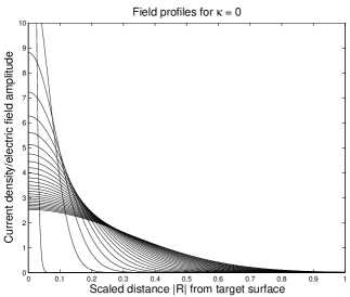
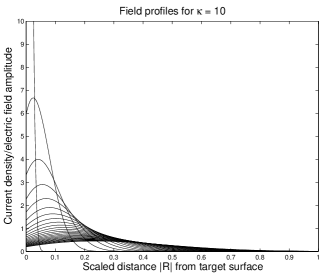
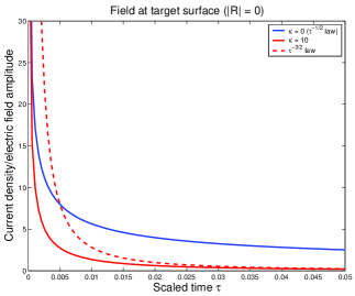
Figure 1: Illustration of the early time evolution of the surface density depth profile from the target surface for nonmagnetic (left) and magnetic (center) targets, beginning from a delta-function initial condition (perfect step function pulse termination). Distance $R=r/L$ is scaled by the target size, time $\tau=t/\tau_{D}$ by the diffusion time, so that $\kappa$ here corresponds $\kappa_{n}\sqrt{\tau_{c}}$ in (11), and is essentially the permeability contrast $(\mu-\mu_{b})/\mu_{b}$. The profiles are plotted for a sequence of 26 equally spaced scaled times $10^{-4}\leq\tau\leq 0.05$ (earlier times corresponding to narrower profiles). The nonmagnetic profile exhibits a pure Gaussian spreading into the target interior, while the magnetic profile is much more complex due to the surface magnetic boundary condition. Its maximum is pushed inwards from the boundary, and decays more rapidly with time. The right plot shows the time trace for the current density at the surface, $R=0$, and is essentially the profile $H(\kappa\sqrt{\tau})$, equation (14), which appears in the measured voltage (11). For $\kappa=0$ (solid blue line) the $\tau$-dependence follows an exact $1/\sqrt{\tau}$ power law. For $\kappa>0$ (solid red line) the $\tau$-dependence crosses over from the identical $1/\sqrt{\tau}$ form at early-early time to the $1/\tau^{3/2}$ power law (dashed red line) at late-early time [the asymptotic forms displayed in (14)].

II-B Complementary early time modeling

For a rapidly terminated transmitter pulse, the external electric field, and induced voltage, display an early time power law divergence [4, 5] (saturating at very early time only on the scale of the off-ramp time $t_{r}$. The boundary between the intermediate (multi-exponential) and late time (mono-exponential) regime occurs at the diffusion time scale

$$\tau_{D}=L^{2}/D$$ (8)

where $L$ is the characteristic target radius, and $D=c^{2}/4\pi\mu\sigma$ is the EM diffusion constant—this is the time scale required for the initial surface currents to diffuse into the center of the target. The early time regime corresponds to times $t\ll\tau_{D}$ (say, $t<\tau_{D}/100$), beginning deep into the multi-exponential regime where many (e.g., hundreds of) modes are excited. In this regime, for nonpermeable, or weakly permeable targets ($\mu\simeq\mu_{b}$), one obtains the simple power law prediction prediction [4]

$$V(t)=V_{e}/t^{1/2},\ t\ll\tau_{D},$$ (9)

with all of the target and measurement parameters encompassed by the single amplitude $V_{e}$, whose computation requires the solution of a certain Neumann problem for the Laplace equation in the space external to the target.

For permeable targets, a new magnetic time scale

$$\tau_{\mathrm{mag}}=\tau_{D}(\mu_{b}/\mu)^{2}$$ (10)

emerges. For ferrous targets, $\mu/\mu_{b}=O(10^{2})$, and $\tau_{\mathrm{mag}}/\tau_{c}=O(10^{-4})$ is tiny. The early time voltage then has a more complex magnetic surface mode structure,

$$V(t)=\sum_{n=1}^{\infty}V_{n}^{e}H(\kappa_{n}\sqrt{t})$$ (11)

where the $\kappa_{n}$ are surface mode eigenvalues, and the mode time trace profile

$$H(s) = \frac{1}{\sqrt{\pi}s}-e^{s^{2}}\mathrm{erfc}(s)$$ (14)

$$\approx \left\{\begin{array}[]{ll}\frac{1}{\sqrt{\pi}s},&s\ll 1\\ \frac{1}{2\sqrt{\pi}s^{3}},&s\gg 1,\end{array}\right.$$

where $\mathrm{erfc}(s)$ is the complementary error function, interpolates between a $1/t^{1/2}$ power law at early-early time, $t\ll\tau_{\mathrm{mag}}$, and a $1/t^{3/2}$ power law at late-early time, $\tau_{\mathrm{mag}}\ll t\ll\tau_{D}$. For large ferrous targets, this latter interval is very large, and may, in fact, accurately represent the signal over nearly the entire measurement interval (see Sec. IV).

Figure 1 illustrates the important features of the early time modeling, including the complex evolution of the surface current depth profile [which extends $H(s)$ to a function of both time and space [5]] that ultimately gives rise to the externally measured voltage (11).

The surface modes are special surface current profiles (two such patterns are shown in Fig. 12 below) that, instead of decaying exponentially, evolve according to the universal function $H(s)$. They and the $\kappa_{n}$ are solutions to an eigenvalue problem defined on the surface of the target [5]. They may be determined analytically only for spherical targets, where one finds

$$\kappa_{l}=l/\sqrt{\tau_{\mathrm{mag}}},\ l=1,2,3,\ldots,$$ (15)

each $(2l+1)$-degenerate, with $\tau_{\mathrm{mag}}=4\pi\sigma\mu_{b}^{2}a^{2}/\mu c^{2}$, where $a$ is the radius. The surface current patterns are controlled by the spherical harmonics of order $l$. The amplitudes $V_{n}^{e}$ again require a solution to an external Laplace-Neumann problem.

Unlike the bulk, exponential modes, under most conditions, only a very few surface modes are excited. The initial surface current pattern more-or-less follows the shape of the magnetic field generated by the transmitter coil. Unless the target is close to the coil, this field is fairly uniform, and the corresponding surface current density is fairly uniform as well, and can then be represented by the first few (two or three) modes. There is a very heavy numerical overhead in computing these modes and their excitation amplitudes, all in pursuit of predicting the rather limited information content of just a few coefficients. Given the success of extending the mean field predictions into the intermediate-early time regime, we have therefore found that it is much more efficient to extend the voltage curve by fitting the data at intermediate times to a one or two term series of the form (11), estimating $\kappa_{n}\approx 1/\sqrt{\tau_{\mathrm{mag}}}$ for the first few modes. Although this precludes quantitative predictions at early-early time, it provides an enormously useful qualitative confirmation that the functional form $H(s)$ accurately describes the data.

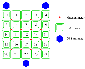
Figure 2: Sketch of NRL TEMTADS array consisting of a $5\times 5$ array of 25 independent, concentric transmitter and receiver coils, numbered from 0 to 24 as shown. Due to rapid decay of signals with target depth, precise (cm level) geometry and placement of the coils (summarized in Table I) can have significant effect on the overall measured voltage amplitude.

Sensor center horizontal separation		40 cm
Transmitter coil center height		4.3 cm
Transmitter diameter		35 cm
Number of transmitter coil windings $N_{T}$		35
Receiver coil center height		0.4 cm
Receiver diameter		25 cm
Number of receiver coil windings $N_{R}$		16

TABLE I: NRL TEMTADS array geometry. The transmitter coil windings are 7.8 cm tall with 0.4 cm thick endcaps on top and bottom. Height is measured from the bottom side of the lower endcap, and the transmitters are then modeled as an idealized 1D square loops at $0.4+3.9=4.3$ cm height. The receiver coils are vertically compact and lie at the bases of the transmitter coils, hence are modeled as idealized 1D square loops at 0.4 cm height.

III TEMTADS platform

III-A Platform geometry

The $5\times 5$ NRL TEMTADS sensor array is sketched in Fig. 2, and its geometrical parameters are summarized in Table I. The loops $C_{T}$ and $C_{R}$ are all modeled as perfect squares with 35 cm and 25 cm edges, respectively. The origin is taken to be at the base of the lower endcap for sensor 12, the positive $x$-axis towards sensor 13, the positive $y$-axis towards sensor 7, and the positive $z$-axis vertically upwards. The transmitter and receiver loop centers then all have $x$- and $y$-coordinates that are multiples of 40 cm. The transmitters are all at $z=4.3$ cm, and receivers are all at $z=0.4$ cm. Target positions and orientations quoted in later sections are all defined relative to this frame of reference.

The precise overall voltage amplitudes, required at least for initial verification of the instrument calibration, turn out to be surprisingly sensitive to small changes in these numbers. The scattered fields are approximately dipolar, and the voltage therefore decreases roughly as $1/d^{6}$ with depth $d$. For example, therefore, a 1 cm error for a 30 cm deep target then leads to a 20% error in the voltage amplitude. A consistent systematic error of this magnitude, in fact, is what led us to discovering the existence of the endcaps, and the vertical offset between the transmitter and receiver loops.

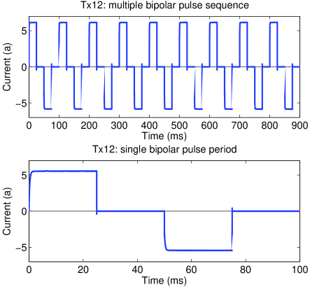
Figure 3: TEMTADS transmitter current bipolar pulse waveform. Top: multiple periods. Bottom: single 100 ms period.

III-B Transmitter waveform

The TEMTADS bipolar pulse sequence is shown in Fig. 3. Each pulse is $t_{p}=25$ ms long, followed by a 25 ms measurement window. An adequate model of the pulse waveform is the form:

$$I(t)=\left\{\begin{array}[]{ll}I_{\mathrm{max}}(1-e^{-t/\tau_{1}}),&0<t\leq t_{p}\\ I_{\mathrm{max}}[1-(t-t_{2})/t_{r}],&t_{2}<t\leq t_{p}+t_{r}\end{array}\right.$$ (16)

with exponential onset time constant $\tau_{1}=0.33$ ms, off-ramp time $t_{r}=10\ \mu$s, and current amplitude $I_{\mathrm{max}}=5.7\pm 0.3$ a. This form misses some detailed multi-exponential behavior during the pulse onset that can be shown to have negligible effect on the excitation coefficients. The second half of the full bipolar pulse, beginning at $t=2t_{p}$, is the same as the one above, but inverted. The functional forms in (16) are simple enough that analytic forms for the current coefficients (4) may be computed straightforwardly.

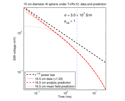
Figure 4: Data and theory for a 15 cm diameter aluminum sphere with center lying 16.5 cm below the center of sensor 12 (see Fig. 2), which is also the only active sensor. The solid red line is the data, the dashed red line the prediction from the exact analytic solution for the sphere, the dotted red line is the mean field prediction (based on 232 modes), and the dashed black line is the early time $1/\sqrt{t}$ power law. The 1.03 overall multiplier listed in the legend has been applied to the data to optimize the fit, and is well within the expected 10% fluctuation in the TEMTADS current amplitude. The vertical dashed line marks the rough division between the early time and multi-exponential ($\lesssim 100$ modes) regimes, and it is seen that the mean field prediction is valid well into the early time regime. The slight deviation of the data from the analytic prediction at very early time, $t<0.1$ ms, is likely an instrument saturation effect (seen much more clearly in Fig. 5, beginning roughly at the same voltage level).

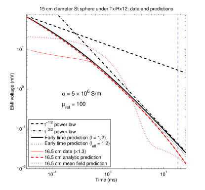
Figure 5: Data and theory for a 15 cm diameter steel sphere with center lying 16.5 cm below the center of sensor 12 (see Fig. 2), which is also the only active sensor. The solid red line is the data (which shows clear instrument saturation above a few volts), the dashed red line the prediction from the exact analytic theory solution for the sphere, the dotted red line is the mean field prediction (based on 232 modes). The dashed black line is a two term fit to the early time form (11) using the known values (15), and the dotted black line is a single term fit using $\kappa_{1}$ as a fit parameter. The vertical dashed line marks the rough division between the early time and multi-exponential ($\lesssim 100$ modes) regimes, and is much later here than in Fig. 4 because the EM time scale is proportional to the product $\sigma\mu$, which is an order of magnitude larger here. For reasons described in the text, the mean field prediction has a more complex structure for ferrous targets, and penetrates only to the edge of the early time regime (it is the fact that it is accurate beyond about 20 ms that is the real figure of merit here, as would be more evident if the data extended to later time). The 1.3 multiplier listed in the legend is that applied to the data to optimize the fit, and lies outside the expected 10% fluctuation in the current amplitude. The difference is likely the result of small positioning errors. Sensor saturation is apparent below about 0.5 ms. The late-early time $1/t^{3/2}$ power law is evident in the data, but full convergence to the $1/\sqrt{t}$ early-early time power law is incomplete, and not expected until about 10 $\mu$s.

IV Data comparisons

IV-A Spherical targets

Having described the electromagnetic model, and the platform model required to implement it, we now turn to its validation with real data. We begin with spherical targets, for which exact analytic solutions exist in both the early time [4, 5] and multi-exponential regimes [2]. This allows one to validate the sensor model under conditions where the target model is fully specified.

Figure 4 shows results for a 15 cm diameter aluminum sphere, plotted on both linear and log time scales—the latter much more clearly verifies the asymptotic $1/\sqrt{t}$ early time power law. The agreement is quite remarkable—note that the vertical scale is in millivolts, not an arbitrary scaled unit. The only real fitting parameter is the conductivity, and the chosen value $\sigma=3\times 10^{7}$ S/m is well within the range expected for aluminum. As discussed in Sec. III, the overall pulse-to-pulse transmitter current amplitude is stable only at the 10% level. This leads to an identical uncertainty in the overall voltage amplitude. In the figure, an overall factor of 1.03 has been applied to the data to obtain an optimal fit, well within this uncertainty. The slowest decaying mode for this target is $\tau_{1}=21.5$ ms, so the measurement window here barely enters the late time regime $t\gtrsim\tau_{1}$. The mean field prediction, based on an approximate calculation of the first 232 modes [7, 8], is seen to accurately describe the data well into the early time regime.

The mean field prediction has much more interesting structure for ferrous targets. Due to the nature of the EM boundary conditions in the large permeability contrast limit, rather than computing only the slowest decaying modes, two distinct sets of slow (169 modes in this case, with time constants larger than 3.01 ms) and fast (63 modes in this case, with time constants smaller than 0.74 ms) decaying modes are produced, with large gap between that would only be filled if one pushed the computation to higher order. This is the source of the S-curve-like structure seen in the right panel of Fig. 5. The reduction in the number of slowly decaying modes reduces the accuracy of the theory near the early–intermediate time boundary (as compared to the nonmagnetic case shown in Fig. 4), but the presence of the more rapidly decaying modes at least provides an improved trend at very early time. The slowest decaying mode for this target has a time constant $\tau_{1}=180$ ms, indicating a late time regime an order of magnitude beyond the measurement.

The early time prediction, which follows both the exact solution and the data over a significant fraction of the time interval, deserves some comment. As described in Sec. II-B, to obtain the solid black lines in Fig. 4) the known eigenvalues (15) are used, but the amplitudes $V_{n}^{e}$ are determined (11) by fitting to the data. Only two terms are kept,

$$V(t)=V_{0}\left[(1-\alpha)H\left(\sqrt{t/t_{\mathrm{mag}}}\right)+\alpha H\left(2\sqrt{t/t_{\mathrm{mag}}}\right)\right]$$ (17)

with the known value $t_{\mathrm{mag}}=0.35$ ms, and the amplitude $V_{0}=83$ V, and mixing parameter $\alpha=0.4$ are fit. The one term series $V_{0}=60$ V, $\alpha=0$ provides an adequate, but lower quality fit.

However, a better fit than both of these is provided by a single term series in which one allows the eigenvalue $\kappa_{1}$ to be adjusted. The dotted black line in Fig. 4) shows the result obtained using $\kappa_{1}=l_{\mathrm{eff}}/\sqrt{t_{\mathrm{mag}}}$ with $l_{\mathrm{eff}}=1.2$, along with amplitude $V_{1}^{e}=80$ V. This will be our fitting method of choice for non-spherical targets, where the eigenvalues $\kappa_{n}$ have not yet been computed.

It is worth emphasizing the importance of the fact that analytic functional forms of the type (17) fit the data so well. The log-time plot demonstrates that the data span the full range over which the argument $s$ in (14) interpolates between the two power laws [12]. The data therefore has significant structure through this time range, but this does not reflect any deep structure of the target (beyond the fact that it is ferrous). Quite the contrary: as illustrated in Fig. 1 it represents the dynamics of a laterally very smooth surface current sheet as it begins to penetrate the first centimeter or so into target. The complexity arises strictly from the interplay between the electric and magnetic field boundary conditions at the surface. This serves to confirm that the early time regime provides limited target discrimination ability (again, beyond the fact that it is ferrous).

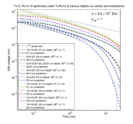
Figure 6: Consolidated plot of data and theory for a range of artificial aluminum prolate spheroidal targets, centered under Tx/Rx12 at various depths and orientations. The dimensions listed in the legend are diameters. Orientation angles indicate symmetry axis declination (toward the center of sensor 11), so that $0^{\circ}$ corresponds to vertical and $90^{\circ}$ to horizontal. The multipliers are again the overall factors applied to the data to obtain optimal agreement with the prediction. The thick dashed lines are the mean field predictions, which show remarkable agreement well into the early time regime, where the onset of the $1/\sqrt{t}$ power law is evident.

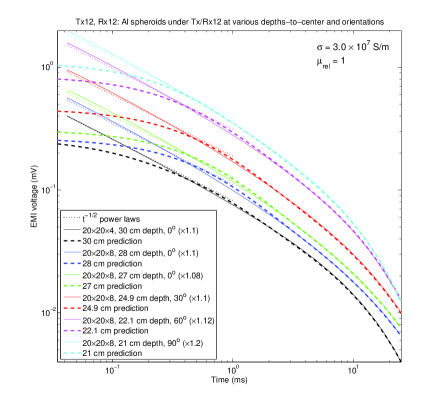
Figure 7: Consolidated plot of data and theory for a range of artificial aluminum oblate spheroidal targets, centered under Tx/Rx12 at various depths and orientations. The thick dashed lines are the mean field predictions, which show remarkable agreement well into the early time regime, where the $1/\sqrt{t}$ power law takes over (dotted lines).

IV-B Prolate and oblate spheroidal targets

Having verified instrument calibration and several other quantitative details under conditions where an exact solution exists, results for spheroidal targets are now presented.

Figure 6 shows a consolidated plot of data and theory for various prolate (elongated) spheroidal aluminum targets at various depths and orientations. Spheroid aspect ratios $a_{z}/a_{xy}$ vary between 2 and 5.

The theoretical plots (thick dashed lines) are the mean field predictions based on the first 232 modes. It is again evident that the mean field predictions are valid well into the early time regime. The multi-exponential time series eventually saturates and falls below the data, but not before the $1/\sqrt{t}$ power law is quite well established. For smaller targets (e.g., the $4\times 4\times 20$ cm and $5\times 5\times 20$ cm spheroids) the mean field prediction can cover nearly the entire measurement window. The multi-exponential time series eventually saturates and falls below the data, but not before the $1/\sqrt{t}$ power law is quite well established. Interpolating between the mean field prediction and this power law clearly enables one to accurately match the data over the full range (this will be demonstrated more quantitatively in the inversion experiments described below).

It is apparent that most of the target discrimination information occurs at intermediate to late time. The traces are all more-or-less parallel at early time, and variations in the overall amplitude from from variation in depth, size or geometry of the target are not distinguishable. On the other hand, at later time, the traces for smaller targets (e.g., again, the $4\times 4\times 20$ cm and $5\times 5\times 20$ cm spheroids) drop off much more quickly than those of larger targets.

There are also interesting dependencies on target orientation in this regime (green, red, magenta, and cyan curves in the upper part of the plot for the $10\times 10\times 20$ cm spheroid [13]). For a vertical target, the excited modes are dominated by currents that circulate around the symmetry axis, while for a horizontal target the currents tend to circulate along it. The horizontal target mode has a slower decay rate (time constant $\tau_{h}=13.7$ ms vs. $\tau_{v}=12.0$ ms), and couples differently to the transmitted field, and this is visible in the later-time traces.

Identical conclusions are evident from the data on oblate (discus-like) spheroidal aluminum targets (aspect ratios $\alpha=0.2,0.4$) shown in Fig. 7. Here we have overlayed segments of $1/\sqrt{t}$ power law on each curve, explicitly demonstrating successful interpolation (with, perhaps, 5–10% errors in the overlap regime).

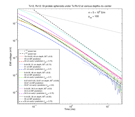
Figure 8: Consolidated plot of data and theory for a range of steel prolate spheroidal targets, centered under Tx/Rx12 at various depths and orientations. The thick dashed lines are the early time predictions, which show remarkable agreement over nearly the entire measurement window. The latter take the form (11) with a single term, in which the amplitude $V_{1}^{e}$ and eigenvalue $\kappa_{1}=l_{\mathrm{eff}}/\sqrt{\tau_{\mathrm{mag}}}$ are adjusted to optimize the fit. Here $\tau_{\mathrm{mag}}$ is defined by (10) and (8), with the choice $L=\min\{a_{xy},a_{z}\}=a_{xy}$. The mean field predictions are shown by the dotted lines. If extended over the full time interval, they also would display the S-curve behavior seen in Fig. 5. For these smaller targets, their region of validity begins only at later times where the signal levels are falling into the noise floor. The early time regime therefore encompasses almost the full range of useful data.

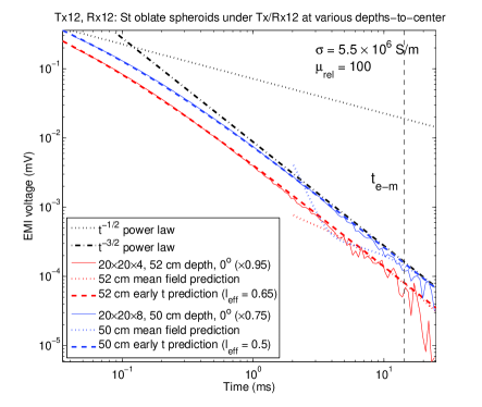
Figure 9: Consolidated plot of data and theory for a range of steel oblate spheroidal targets, centered under Tx/Rx12 at various depths and orientations. The thick dashed lines are the early time predictions, which show remarkable agreement over nearly the entire measurement window. The latter take the form (11) with a single term, in which the amplitude $V_{1}^{e}$ and eigenvalue $\kappa_{1}=l_{\emph{eff}}/\sqrt{\tau_{\mathrm{mag}}}$ are adjusted to optimize the fit. Here $\tau_{\mathrm{mag}}$ is defined by (10) and (8), with the choice $L=\min\{a_{xy},a_{z}\}=a_{z}$. The mean field predictions are shown by the dotted lines. For these smaller targets, their region of validity again begins only as the signal levels are falling into the noise floor. The early time regime ($t<t_{\mathrm{e\mbox{-}m}}$) encompasses nearly the full range of useful data.

The dependence on orientation is much stronger for oblate spheroids (green, red, magenta, and cyan curves for the $20\times 20\times 8$ cm spheroid [13]). Because it is being “squeezed” vertically, the horizontal target (discus on edge) mode now has significantly faster decay rate than vertical target (discus lying flat) mode (time constant $\tau_{h}=13$ ms vs. $\tau_{v}=24$ ms). Because the the latter mode is not excited at all when the target is horizontal, the $90^{\circ}$ (cyan) curve in Fig. 7 decays much more quickly at late time than the other curves.

In both Figs. 6 and 7 the multipliers used to scale the data for optimal fit appear to have a small ($\sim 10$%) systematic bias that cannot be explained by random variation in the transmitter loop current. A combination of small conductivity and positioning errors is the likely culprit.

Figures 8 and 9 show data and theory for steel prolate and oblate spheroidal targets. As for the steel sphere (Fig. 5), the early time regime dominates, and the mean field results (dotted curves; with S-curve behavior excised in this case so as not to confuse the plots) are valid only over a small part of the time interval where the data is already becoming quite noisy. In most cases, however, the fact that the data is dropping below the early time curve is evident, pointing to the necessity of a multi-exponential description. As before, these predictions actually push quite deeply into the early time regime, but the measurement window, and instrument dynamic range, are such as to strongly limit the information content of the multi-exponential part of the signal.

V Inverse problem for spheroidal targets

We have so far described applications of the early time and exponential models to the forward problem, in which detailed model predictions for a known target are compared to data. Having demonstrated the quantitative success of the models for this problem, we now turn to the inverse problem, in which some set of target characteristics is treated as unknown, and one attempts to determine them by searching for the target model whose predictions best match the data. We have previously presented solutions to the inverse problem using noise corrupted simulated data [6]. Here we will base the inversions on the TEMTADS data.

Of particular interest are ambiguities in the data, i.e., target properties that are poorly constrained by a particular data set, either due to poor data quality (e.g., noise), or due to fundamental trade-offs between certain parameters that exist even for essentially perfect data. We will see, for example, that it is very difficult to simultaneously determine target depth, size, and conductivity. We will also see that the enormous differences seen between magnetic and nonmagnetic target data in Sec. IV give rise to similar differences for the inverse problem.

V-A Objective function

Inverse problems are generally formulated as the solution to the following optimization problem. Let ${\bf m}\in M$ be a vector of forward model parameters spanning a model space $M$, in our case the space of target and sensor platform parameters that define the forward problem. Let ${\bf d}$ be the measured data vector, in our case the set of voltage time series corresponding to a given set transmitter-receiver combinations and platform positions. Let ${\bf d}_{\mathrm{pred}}({\bf m})$ be the forward model prediction for the data given a model ${\bf m}$. For a perfect model and perfect data, there should be a unique model ${\bf m}_{0}$ for which ${\bf d}_{\mathrm{pred}}({\bf m}_{0})={\bf d}$. In the presence of noise, and/or an incomplete model (e.g., real UXO are not ideal spheroids), such an exact match is not achievable, and we instead seek an optimal solution rather than a perfect solution.

The sense in which a solution is optimal is defined by an objective function $F({\bf m}|{\bf d})$, which, e.g., vanishes if ${\bf d}_{\mathrm{pred}}={\bf d}$, but more generally attains a minimum value ${\bf m}_{0}$ in the space of available models:

$${\bf m}_{0}=\arg\min_{{\bf m}\in M}F({\bf m}|{\bf d}).$$ (18)

Finding this minimum entails a search over the space $M$, and there may be multiple local minima that interfere with the discovery of the absolute minimum. It is generally the case, as well, that the problem is under-determined, and an entire subspace of different ${\bf m}$, for example, may very nearly achieve the same minimum. To some degree, such ambiguities can be controlled using a priori constraints (e.g., on a target’s permitted range of depths or conductivities), effectively biasing $F({\bf m}|{\bf d})$ toward a preferred set of solutions. The danger, of course, is that this blinds one to targets disagreeing with this bias, and ${\bf m}_{0}$ may end up being vastly different from the truth. We will see examples of this below.

In what follows, we will use the following form of objective function:

$$F({\bf m}|{\bf d})=\sum_{k=1}^{N_{t}}W_{k}\left[\frac{V_{\mathrm{meas}}(t_{k})}{V_{\mathrm{pred}}(t_{k};{\bf m})}-1\right]^{2}+F_{\mathrm{prior}}({\bf m}),$$ (19)

in which $t_{k}$, $k=1,2,\ldots,N_{t}$ are the measurement platform time gates, $V_{\mathrm{meas}}$, $V_{\mathrm{pred}}$ are the measured and predicted voltages, and $F_{\mathrm{prior}}$ contains any prior constraints. The weights $W_{k}$ may be used to fine tune the weighting given to data in the different time regimes, for example suppressing noise-dominated time gates. The ratio $V_{\mathrm{meas}}/V_{\mathrm{pred}}$ is used (adopting, basically, a logarithmic rather than a linear voltage scale), in place, e.g., of a more conventional mean square error $(V_{\mathrm{meas}}-V_{\mathrm{pred}})^{2}$, in order to give more democratic weight to early and later-time regimes. Specifically, signals may be orders of magnitude weaker at later time, but it will be seen that the multi-exponential decay still contains key target identification information not present at early time. In addition, $V_{\mathrm{pred}}$ is placed in the denominator because noise effects may easily induce sign changes in $V_{\mathrm{meas}}$ at later time, which would produce singularities in $V_{\mathrm{pred}}/V_{\mathrm{meas}}$.

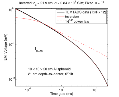
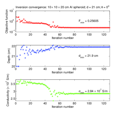
Figure 10: Inversion experiment using TEMTADS data for a $10\times 10\times 20$ cm prolate spheroid, using the objective function (19). Prior information is incorporated in that only the parameters ${\bf m}=\{\sigma,d,t_{\mbox{e-m}}\}$ are permitted to vary. Target geometry and orientation (symmetry axis vertical) are fixed, and the transmitter current amplitude is fixed at 5.5 a. The upper plot shows the data (thick black line—the same as the green curve in Fig. 6) and the remarkably accurate optimal fit (solid red line to the right of $t_{\mbox{e-m}}$; dashed red line to its left). The lower plot shows the convergence of $F,\sigma,d$ with iteration number. Note the two-stage convergence, in which $d$ equilibrates first, followed by the ‘weaker’ parameter $\sigma$.

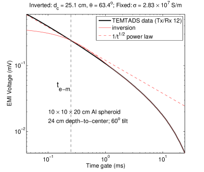
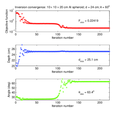
Figure 11: Second inversion experiment using TEMTADS data for a $10\times 10\times 20$ cm prolate spheroid, using the objective function (19). The parameters ${\bf m}=\{d,\theta,t_{\mbox{e-m}}\}$ are now permitted to vary. Target geometry is fixed, the transmitter current amplitude is fixed at 5.5 a, and the conductivity is fixed at the value found in the first experiment (Fig. 10). The upper plot shows the data (thick black line—the same as the magenta curve in Fig. 6) and optimal fit (solid red line to the right of $t_{\mbox{e-m}}$; dashed red line to its left). The lower plot shows the convergence of $F,\theta,d$ with iteration number. The value of $\theta_{\mathrm{min}}=63.4^{\circ}$ is very close to the $60^{\circ}$ ground truth. One sees even more clearly in this figure the initial equilibration of the depth, followed later by the convergence of the tilt angle, which has a much weaker effect on the voltage time series, mostly at later time.

V-B Inversions for aluminum targets

We begin with a set of numerical inversion experiments using the $10\times 10\times 20$ cm aluminum spheroid data (upper curves in Fig. 6). We consider some interesting issues involving tradeoffs between target depth, conductivity, and orientation, which are most clearly elucidated by treating the target geometry (in this case, $a_{xy}=5$ cm radius, aspect ratio $\alpha=a_{z}/a_{xy}=2$) as known. We have performed inversions in which the target geometry also varies (see also Ref. [6]) and found similar effects. We will also use the (highest quality) data only from the pair Tx12-Rx12. In Sec. VI, some results will be shown using multiple Tx/Rx pairs. The inversion code uses the standard simplex method (which ‘walks’ its way toward a local minimum, in sequentially decreasing steps), that does not require any gradients of the objective function. More sophisticated search methods, that may operate more efficiently, will be left for future work.

The transition between the early-time and multi-exponential regimes for non-magnetic targets is treated as follows. One of the inversion parameters is taken to be a crossover time $t_{\mathrm{e\mbox{-}m}}$, and for a given value, the predicted voltage takes the form

$$V_{\mathrm{pred}}(t)=\left\{\begin{array}[]{ll}V_{\mathrm{MF}}(t),&t>t_{\mathrm{e\mbox{-}m}}\\ V_{\mathrm{MF}}(t_{\mathrm{e\mbox{-}m}})(t/t_{\mathrm{e\mbox{-}m}})^{-1/2},&t<t_{\mathrm{e\mbox{-}m}},\end{array}\right.$$ (20)

in which $V_{\mathrm{MF}}(t)$ is the direct mean field prediction based on the remaining parameters in ${\bf m}$ [14].

In a number of numerical experiments, it was found that if the target conductivity $\sigma$, the depth $d$, and the tilt angle $\theta$ are all permitted to vary, the inversion is very unstable. Specifically, varying the tilt changes the signal decay rate at later time (reflecting differences in the decay rates of the excited modes). However, so does varying the conductivity, and the two effects can very nearly be made to cancel, so long as the depth is adjusted slightly to maintain the observed overall signal amplitude. The result is a solution ${\bf m}_{0}$ with unphysical values of all three parameters. In realistic scenarios, one would then have to include in $F_{\mathrm{prior}}$ terms that constrain, for example, the conductivity to in a range of acceptable values for aluminum.

 

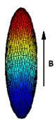
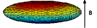
Figure 12: Early time surface current flows depending on relative orientation of the magnetic field for a 4:1 prolate spheroid. Plotted is the stream function $\psi$ associated with two of the early time surface modes whose level curves are the stream lines of the surface current (circulating clockwise around blue patches, counterclockwise around red patches). The characteristic radius $r_{\mathrm{eff}}$ associated with a mode is essentially the (half) distance between extrema of $\psi$ (red and blue regions). The diffusion of the surface current sheet into the target, at any given point on the surface, is shown in Fig. 1 for different values of $\kappa=(\mu/4\pi\sigma)^{1/2}cr_{\mathrm{eff}}$.

Since, for the data dealt with in this section, we have complete ground truth, we proceed in a slightly different fashion. We begin by determining an optimal value of the conductivity from one of the data sets using the known value of the tilt angle (as well as the target horizontal position). The depth and crossover time are permitted to vary as well. The results are shown in Fig. 10, where a value $\sigma=2.84\times 10^{7}$ S/m is found. Using a different value of $\sigma$ is found to significantly change the inversion result for the tilt angle.

Note that convergence of the inversion takes place in two stages. The depth equilibrates first, due to the strong $1/d^{6}$ dipolar dependence of the overall voltage amplitude. Once a reasonable value for $d$ emerges, the more subtle conductivity-induced changes in the voltage curve shape (mainly at later time) can be productively optimized.

Note also that the inverted depth $d_{\mathrm{min}}=21.9$ cm differs slightly from the 21 cm ground truth value. This may partially be due to experimental error, but is likely also due to the $\sim$10% uncertainty in the transmitter current amplitude $I_{\mathrm{max}}$ (see Sec. III-B) which has been fixed at the value 5.5 a. Inversion experiments have been performed in which $I_{\mathrm{max}}$ is also treated as a free parameter, but this is also found to be highly unstable. Specifically, the voltage signal changes very little if $I_{\mathrm{max}}$ is varied, while at the same time adjusting the target depth $d$—both mainly affect the overall amplitude of the voltage time series, not its shape [15]. For the same reason, here and in experiments described below, this ambiguity has very little effect on the inverted values of most other parameters, specifically those that indeed impact the shape of the time series.

With an accurate conductivity value now in hand, in our second inversion experiment, we fix the former and invert for the tilt angle [16]. As seen in Fig. 11, this indeed produces an inverted $\theta_{\mathrm{min}}$ very close to the $60^{\circ}$ truth. The two-step nature of the convergence is seen here as well. Similar experiments (not shown) using the $30^{\circ}$ and $90^{\circ}$ tilt data (red and cyan curves, respectively, in Fig. 6) produce equivalent results. The inverted depth $d_{\mathrm{min}}=25.2$ cm differs only slightly from the 24.4 cm ground truth.

We have performed inversions as well using the $20\times 20\times 8$ cm oblate spheroid data shown in Fig. 7) which yield very similar results (not shown). One again fits the conductivity (and depth) using the $0^{\circ}$ tilt data (green curve in Fig. 7), and then uses this value to invert for tilt angle (and depth) using the other data sets. One again finds delicate features where a slightly incorrect conductivity value leads to a highly inaccurate tilt angle. The problem actually appears to be somewhat worse in this case because of the early time crossover time $t_{e\mbox{-}m}$ occurs relatively earlier for oblate geometries, increasing the model misfit for the given number of modes (232).

 

 

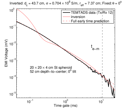
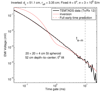
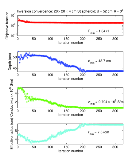
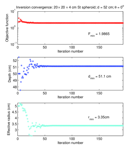
Figure 13: Two inversion experiments using TEMTADS data for a $20\times 20\times 4$ cm steel oblate spheroid, using the objective function (19). Rather than producing a simple power law, the early time theory now produces the nontrivial ‘error function’ series (11) and (14), modeled here as a single term with optimized value of the effective radius $r_{\mathrm{eff}}$ (solid red line in the upper plots). The target orientation is held fixed (symmetry axis vertical). Left hand plots: the depth, conductivity, and effective radius are permitted to vary. The resulting over-fit of the later-time noise produces unphysical values of all three. Right hand plots: the conductivity is now fixed at a physically reasonable value $\sigma=3\times 10^{6}$ S/m. The depth, conductivity, and effective radius now converge to physically reasonable values as well.

 

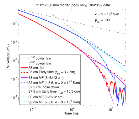
Figure 14: TEMTADS data (solid lines) and theoretical fits (dashed lines) taken for a 60 mm (left) and 81 mm (right) mortar body targets lying flat (red and magenta curves) and nose-up vertical (blue and cyan curves). The early time fits, based on (21) and (22) with $\mu=100$ and $\sigma=5\times 10^{6}$ S/m, produce the very reasonable effective diameters $d_{\mathrm{eff}}=2r_{\mathrm{eff}}$ (see the illustrations in Fig. 12) as indicated in the legends. The length listed at the beginning of each legend entry is the target depth (ground truth for the data and early time curves; fitted value for the mean field curves). The mean field predictions (solid magenta and cyan curves), using these same parameters, properly extend the early time curves but completely fail to fit the data. Lowering the conductivity by more than an order of magnitude accurately mimics the increased rate of decay (dashed magenta and cyan curves), but the overall voltage amplitude is incorrect (as indicated by the applied multipliers in the legend). As described in the text, and in Fig. 15, the correct explanation for the discrepancy is the finite (0.5–1 cm) mortar shell thickness.

V-C Inversions for steel targets

We next present inversions based on the data shown in Fig. 9 for steel oblate spheroidal targets. These turn out to serve as an illustration of another set of inversion pitfalls one may encounter, in this case depending on how one balances prior knowledge in the presence of noisy data in the later time regime.

Since the early time behavior of ferrous targets is much more complicated than that for nonmagnetic targets, in addition to the crossover time $t_{\mathrm{e\mbox{-}m}}$, one must provide an appropriate parametrization of the magnetic surface mode series (11) and (14) [5]. As described in Sec. II-B, replacing the series by a single term with effective parameters is found to provide the best fit. For reasons that will become evident below, we parameterize it in the form

$$V_{e}(t)=V_{0}^{e}H(\sqrt{t/\tau_{e}}),$$ (21)

where

$$\tau_{e}=\frac{1}{\kappa^{2}}=\frac{4\pi\sigma}{\mu c^{2}}r_{\mathrm{eff}}^{2},$$ (22)

with $r_{\mathrm{eff}}$ an effective early time target radius. This parameter, derived as previously from the early time eigenvalue $\kappa_{n}$, reflects the primary length scale of the surface currents for a given mode, and decreases as $n$ increases and the geometric complexity of the mode increases. This length scale may be thought of as the diameter of the target along the direction of the magnetic field that primarily serves to excite the mode. For example, currents circulating around the symmetry axis $a_{z}$ are generated by a vertical magnetic field (left panel of Fig. 12), and $r_{\mathrm{eff}}$ is then found to be comparable to $a_{z}$. For magnetic field orthogonal to $a_{z}$ the currents circulate up one side of the symmetry axis and down the other (right panel of Fig. 12), and $r_{\mathrm{eff}}$ is found to be comparable to the radius $a_{xy}$.

As a consequence the length $a_{z}$ will be reflected in the early time data when $a_{xy}$ is what would observed in a corresponding visual inspection of the target from the point of view of a transmitter-receiver above. Correspondingly, when the target is laid with symmetry axis horizontal, $a_{xy}$ will be exhibited when a visual inspection would clearly see both $a_{xy}$ and $a_{z}$. These observations will be confirmed by the data below.

Analogous to the inversion shown in Fig. 10, in Fig. 13 we show inversions for the parameters $d,\sigma,t_{\mathrm{e\mbox{-}m}},r_{\mathrm{eff}}$ with tilt angle fixed at the $0^{\circ}$ ground truth value, and $\mu=100$. As can be seen, the crossover time $t_{\mathrm{e\mbox{-}m}}\simeq 10$ ms lies in a regime where noise effects are becoming significant. In particular, in this case the noise happens to induce a sharper downturn in the signal in the multi-exponential regime than is case for the true signal. In attempt to fit this, the inversion on the left unphysically suppresses the conductivity ($\sigma_{\mathrm{min}}=7.04\times 10^{5}$ S/m), and compensates with an unphysically large effective radius ($r_{\mathrm{min}}=7.37$ cm, much larger than the 2 cm half-thickness of the discus). This keeps the product $\sigma r_{\mathrm{eff}}^{2}$ in (22) essentially fixed, thereby maintaining a good fit in the early time regime. Note that the depth $d_{\mathrm{min}}=43.7$ cm also differs substantially from the 52 cm ground truth.

In order to avoid this overfit of the noise, the right hand side of Fig. 13 shows the superior result obtained by fixing the conductivity at the physically reasonable value $\sigma=3\times 10^{6}$ S/m, with the results $r_{\mathrm{min}}=3.35$ cm and $d_{\mathrm{min}}=51.1$ cm.

The main lesson here is that significantly different information (specifically, different combinations of conductivity with other parameters) is contained in the early time and later time regimes for ferrous targets, and there are large parameter ambiguities in the absence of good data in both. For ferrous targets, the more rapid $1/t^{3/2}$ dominant decay in early time leads to much smaller signals, hence degraded data, in the multi-exponential regime. Parameters relying on the latter will therefore be more poorly determined, and one may be forced to apply a larger set of prior knowledge constraints than for nonmagnetic targets. Since real UXO targets are usually ferrous, this lesson has important practical implications.

VI Some results for Real UXO targets

We turn finally to some initial inversion results for real UXO targets, namely 60 mm and 81 mm mortar bodies, selected for their near-spheroidal shape. The former has a 6 cm diameter, and is approximately 13 cm long; the aspect ratio is therefore taken as $\alpha=2$. The latter has an 8.1 cm diameter and is approximately 25 cm long; the aspect ratio is therefore taken as $\alpha=3$. Real UXO are not ideal spheroids, but we will see that key target discrimination information can be obtained by comparing their electromagnetic responses to those of spheroids with similar geometry.

Data and theoretical fits for both UXO are shown in Fig. 14. The most important observation is that, with the assumptions $\sigma=5\times 10^{6}$ S/m and $\mu=100$, the early time curves for the two orientations (vertical and flat) produce excellent fits, and estimates for the effective radius that accord very nicely with the discussion in Sec. V-C (and Fig. 12): for the vertically oriented mortars, $r_{\mathrm{eff}}=10.5,\ 14.7$ cm are indeed comparable to the mortar half-lengths, while for ‘flat’ mortars, $r_{\mathrm{eff}}=3.7,\ 3.9$ cm are comparable to their radii. Note that these inferences are independent of the target depth (which, to leading order, affects only the amplitude $V_{0}^{e}$).

The next observation is that, contrary to the early time fit, the mean field predictions (dashed blue and red lines in Fig. 14) fail to fit the data. Thus, although they provide a logical extension of the early time curves [17], the data follow a much more steeply decaying path. As indicated by the red and magenta dashed lines, the decay can be fit using much smaller (by factors of 20–50) conductivities. However, these unphysically small effective values are also unphysically orientation dependent, and give similarly inconsistent values for the overall voltage scales (hence the $\times 4$–$\times 7$ fudge factor multipliers listed in the figure legends).

The origin of these modeling discrepancies is that the finite mortar shell thickness (in the 0.5–1 cm range) has not been accounted for. To illustrate this, in Fig. 15 exact analytic results for a hollow sphere are shown. The results there confirm the rapid increase in the mode decay rates with decreasing shell thickness (left panel), and the resulting early breakaway of the voltage curves from the early time result (right panel). The breakaway time scales with the shell thickness as $t_{X}\sim w_{\mathrm{shell}}^{2}/D$, where $D=c^{2}/4\pi\mu\sigma$ is the electromagnetic diffusion constant (see Sec. II-B). With the given values, this relation may be put in the form:

$$\frac{t_{X}}{1\ \mathrm{ms}}\sim\left(\frac{w_{\mathrm{shell}}}{1.3\ \mathrm{mm}}\right)^{2}.$$ (23)

In Fig. 14, ones observes $t_{X}\sim 2$–3 ms, which indeed places $w_{\mathrm{shell}}$ in the right range (and is consistent as well with the $\alpha_{h}=0.8$, 0.85 curves—hence $w_{\mathrm{shell}}=0.3$–0.5 cm—in Fig. 15).

To summarize, the early time fits provide direct estimates of the target geometry, while the breakaway time $t_{X}$ away from the early time extrapolation (as well as the solid spheroid mean field prediction), provide direct estimates of the UXO shell thickness. These are key parameters in target identification. Quantifying the latter would require an enhancement of the mean field code to deal explicitly with hollow spheroids. This can be done with modest effort, and will be considered for future work.

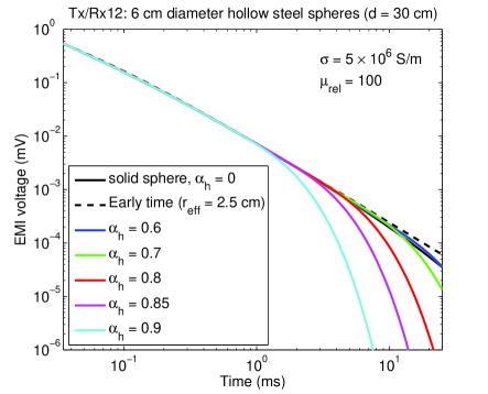
Figure 15: Exact analytic TDEM voltage predictions for a sequence of hollow steel spheres, including the solid sphere ($\alpha_{h}=0$, solid black line). Since the surface geometry of all targets is identical, the same early time curve (dashed line) fits all data sets. However, the multi-exponential regime begins earlier for thinner-shelled targets.

 

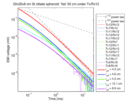
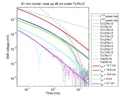
Figure 16: Data (thin solid and dashed lines) and early-time model fits (thick solid lines) for two fixed steel targets using different Tx/Rx combinations (with labeling shown in Fig. 2). Left: $20\times 20\times 8$ cm oblate spheroid. Right: 81 mm mortar body. For these symmetrically placed targets, the solid and dashed curve pairs of each color (e.g., Tx7/Rx12 and Tx11/Rx12; Tx11/Rx13 and Tx7/Rx17) should be degenerate, and this is indeed observed. In both cases the early-time effective target radius (listed in the legend) is seen to vary with ‘look angle’ in a way consistent with the target and measurement geometry. Note that the breakaway time (23) continues to be observable in a number of the 81 mm voltage traces (and continues to be notably absent in the solid spheroid traces). The cusp-like feature in the 81 mm Tx11/Rx13 and Tx7/Rx17 traces (solid and dashed cyan curves) actually represents a sign change in the voltage, as discussed in the text.

VI-A Information content of multiple Tx-Rx combinations

As described in the previous subsection, the early time prediction provides an effective orientation-dependent target radius. For a given buried target, the orientation is fixed, and one seeks other ways of extracting this information. Here one may take advantage of the array degrees of freedom available with the TEMTADS platform: each Tx-Rx pair effectively provides a different ‘look’ at the target. In Fig. 16 we show such data for $20\times 20\times 8$ cm oblate steel spheroid (left panel), and the 81 mm mortar (right panel). In each case the targets are centered (50 cm and 48 cm, respectively) below Rx/Tx12, with their symmetry axes vertical. See Fig. 2 for the labeling.

Note that if the transmitter and receiver coils were identical then, by complementarity, the Tx(m)/Rx(n) response would coincide with that of Tx(n)/Rx(m). The fact that they are somewhat different (see Table I) explains, for example, the small differences between the sets of green and blue curves (e.g., Tx7/Rx12 vs. Tx12/Rx7 or Tx17/Rx12 vs. Tx12/Rx17). On the other hand, if two sets of Rx/Tx pairs are symmetrically placed relative to the (axially symmetric) target, then the responses should be identical (e.g., Tx7/Rx12 vs. Tx11/Rx12 or Tx11/Rx13 vs. Tx7/Rx17), and this is indeed observed.

To leading order, the actual time series is a superposition of the horizontal and vertical early time magnetic surface modes (Fig. 12), and one expects that a fit to a single value of $r_{\mathrm{eff}}$ will then find values that interpolate between the two. This is indeed, for the most part, seen to be the case. For the combination Rx12/Tx12 (red lines), the effective radius is indeed comparable to the ‘vertical half-height’ of the target (4 cm, vs. $r_{\mathrm{eff}}=4.3$ cm for the oblate spheroid; 12 cm vs. $r_{\mathrm{eff}}=14.7$ cm for the 81 mm mortar).

So long as either Rx12 or Tx12 is used (e.g., green and blue curves in Fig. 16), $r_{\mathrm{eff}}$ remains comparable to (or even larger than) its Rx12/Tx12 value. For Tx12, this is because the same dominant magnetic surface mode is being excited, irrespective of which receiver is used to observe it. For Rx12 the same argument proceeds through complementarity: an off-center transmitter will excite more than one surface mode, but the symmetrically placed receiver will see only the symmetrically circulating mode.

However, when both transmitter and receiver are off-center (e.g., cyan and magenta curves in the figure), the effective radius is seen to become comparable to the physical (horizontal) radius of the target (10 cm for the oblate spheroid; 4.05 cm for the mortar). Thus, despite the fact that the overall signal levels drop precipitously as the Tx-Rx separation increases, to the point where the multi-exponential regime becomes unobservable [18], robust target geometry inferences can still be made using this data through the early-time prediction fits. It should also be noted that these fits, being restricted to the early time regime, entail adjustment of the single parameter $r_{\mathrm{eff}}$ (or $\kappa$), and so do not require a sophisticated inversion scheme.

There is one feature of the 81 mm mortar data that deserves further comment. The Tx11/Rx13 and Tx7/Rx17 (cyan curves in the left panel of Fig. 16) display an unusual cusp feature at about 0.3 ms. Since the magnitude of the voltage is being plotted, this actually corresponds to a node in the response, i.e., a sign reversal of $V(t)$. The easiest way to understand this effect is to note that a target close to Tx12 will generate a net downward-pointing magnetic field through Rx13. However, as the target depth increases, the field becomes net upward-pointing, reversing the sign of the flux, and hence of the induced voltage. In this picture, a node in the response occurs as a function of target depth, but a similar argument would also produce a node as a function of time due to exchange of dominance of two early-time mode contributions. Vertical variation of the applied magnetic field will always produce higher order modes (with more complex spatial structure than those shown in Fig. 12) with faster decay rates, and near the critical depth the multiple contributions sum to produce a zero crossing.

VII Summary and conclusions

The results presented in this paper demonstrate the unprecedented accuracy available from our first principles, physics based models covering the entire measurement window, from the early time multi-power law regime, all the way through the multi-exponential regime to the late time mono-exponential regime. Prior to the mean field code’s current iteration [7, 8], the number of accurately computed modes used to describe the multi-exponential regime was limited to perhaps a few dozen [6]. As seen in the results presented, by generating the required overlap of the early time and multi-exponential regimes, this improvement is critical to the success of the validation and inversion tests.

It should be emphasized that the increase in predictive power continues to operate with extremely high numerical efficiency. The creation of the mode data for a given target cannot be performed in real time, but once this data is made available in a database that spans the expected target geometries, its acquisition and use for measurement predictions can be performed in real time—operating at essentially the same speed as predictions using the exact solution for the sphere.

As seen in the figures, the dominant regimes visible in the data depend very strongly on the target size and physical properties. Increasing target size and magnetic permeability expands the early time regime to later physical time. Smaller aluminum targets (e.g., blue lines in Fig. 6) are completely described by the mean field approach over the full time range, while even the smaller steel targets barely enter multi-exponential regime (see Figs. 8 and 9) before the signal fades into the noise floor [19].

Through investigation of inversions it has been shown that different time regimes and different Tx/Rx pairs contain complementary target discrimination information. The most exciting development is the observation that the early time regime, which dominates the steel target response, contains direct information about the target geometry (via the different effective target diameters seen from different ‘look angles’) and the hollow target shell thickness (through the earlier breakaway time to multi-exponential decay for thinner shelled targets). These are key features that will support target identification and clutter rejection.

All of these features, whose quantitative interpretation is enabled by the present models, can be applied to the pursuit of robust target discrimination and identification under more challenging conditions. The code efficiency becomes especially critical for this purpose, as searches through the database for the target whose response best matches the data requires hundreds, or perhaps even thousands, of iterations. In the inversion results presented, these searches presently take several minutes. Further focused improvements in code efficiency could probably reduce this to under one minute.

Peter B. Weichman is a principal research scientist at BAE Systems, Advanced Information Technologies.

References

- [1] See the many documents and links on the Strategic Environmental Research and Development Program (SERDP) website http://www.serdp.org/.
- [2] See, e.g., J. D. Jackson Classical Electrodynamics (John Wiley and sons, New York, 1975).
- [3] P. M. Morse and H. Feshbach Methods of Theoretical Physics, (McGraw-Hill, New York, 1953).
- [4] P. B. Weichman, “Universal early-time response in high-contrast electromagnetic scattering,” Phys. Rev. Lett. 91, 143908 (2003).
- [5] P. B. Weichman, Surface modes and multipower-law structure in the early-time electromagnetic response of magnetic targets, Phys. Rev. Lett. 93, 023902 (2004).
- [6] P. B. Weichman and E. M. Lavely, “Study of inverse problems for buried UXO discrimination based on EMI sensor data,” Proc. SPIE Vol. 5089 Detection Technologies for Mines and Minelike Targets VIII (SPIE, Bellingham, WA, 2003), p. 1139.
- [7] P. B. Weichman, “Chandrasekhar theory of electromagnetic scattering,” arXiv:1108.2239v1 [physics.class-ph].
- [8] P. B. Weichman, “Chandrasekhar theory of electromagnetic scattering from strongly conducting ellipsoidal Targets,” submitted to Phys. Rev. E (2012). arXiv:1206.0975v1 [physics.class-ph]
- [9] B. E. Barrowes, K. O’Neill, T. M. Grzegorczyk, X. Chen, and J. A. Kong, “Broadband analytical magnetoquasistatic electromagnetic induction solution for a conducting and permeable spheroid,”IEEE Trans. Geosci. Remote Sens. 42, 2479–2489 (2004).
- [10] X. Chen, K. O’Neill, T. M. Grzegorczyk, and J. A. Kong, “Spheroidal mode approach for the characterization of metallic objects using electromagnetic induction,”IEEE Trans. on Geosci. Remote Sens. 45, 697–706 (2007).
- [11] B. E. Barrowes, K. O’Neill, T. M. Grzegorczyk, B. Zhang, and J. A. Kong,“Electromagnetic induction from highly permeable and conductive ellipsoids under arbitrary excitation: Application to the detection of unexploded ordnances” IEEE Trans. Geosci. Remote Sens. 46, 1164–1176 (2008).
- [12] This is far less obvious on the linear-time plot, in which only the late-early time power law is clearly visible. The log-time scale is key to elucidating the multi-scale nature of the target electrodynamics.
- [13] For the cm and cm spheroid measurements, the bottom of the target rested on a platform at 31 cm depth, and so the depth-to-center varies with orientation: between 26 cm (horizontal target) and 21 cm (vertical target) for the former; between 27 cm (vertical target) and 21 cm (horizontal target) for the latter.
- [14] In principle, the exact amplitude of could be computed from first principles using the early-time theory [4], but this would necessitate significant computational effort in pursuit of a single coefficient.
- [15] Simultaneous inversions of multiple time series would probably remove most of this particular ambiguity, since different Tx-Rx pairs provide different ‘looks’ at a target that vary significantly relative to one another with depth. This will be a subject of future work.
- [16] Target orientation, of course, is determined by the azimuthal angle as well. However, for a target centered under the Tx/Rx coil, the dependence on is extremely weak (and would be nonexistent for circular coils), and is therefore treated as fixed at the experimental value (along the line joing the centers of Rx/Tx10 and Rx/Tx/14—see Fig. 2). Simultaneous inversions of multiple Tx-Rx pairs would effectively remove this ambiguity as well (cf. footnote [15]).
- [17] Note that for the targets lying flat, the estimated target depths lie only 2 cm from their ground truth values, while for vertical targets there are much larger (7.5 cm and 5 cm) discrepancies. One possible reason for this is the signicant nose-tail asymmetry of the mortars, which will generally bias the effective spheroid center away from the target geometric center.
- [18] Though, for the 81 mm mortar this regime begins earlier, and the accompanying breakaway time , equation (23), continues to be apparent in a number of the voltage traces in the right panel of Fig. 16.
- [19] This signal fading is exacerbated by the more rapid decay of the late-early time signal for steel targets, as compared to the much slower aluminum targets. The latter then have greater tendency to maintain strong signals into the multi-exponential regime (see Figs. 6 and 7). As decribed in Sec. II-B (see especially Fig. 1), this more rapid decay has its orgin in the surface current dynamics, which, in magnetic targets, tends to more quickly push the currents away from the target surface.