Model Selection for Degree-corrected Block Models

Abstract

The proliferation of models for networks raises challenging problems of model selection: the data are sparse and globally dependent, and models are typically high-dimensional and have large numbers of latent variables. Together, these issues mean that the usual model-selection criteria do not work properly for networks. We illustrate these challenges, and show one way to resolve them, by considering the key network-analysis problem of dividing a graph into communities or blocks of nodes with homogeneous patterns of links to the rest of the network. The standard tool for doing this is the stochastic block model, under which the probability of a link between two nodes is a function solely of the blocks to which they belong. This imposes a homogeneous degree distribution within each block; this can be unrealistic, so degree-corrected block models add a parameter for each node, modulating its over-all degree. The choice between ordinary and degree-corrected block models matters because they make very different inferences about communities. We present the first principled and tractable approach to model selection between standard and degree-corrected block models, based on new large-graph asymptotics for the distribution of log-likelihood ratios under the stochastic block model, finding substantial departures from classical results for sparse graphs. We also develop linear-time approximations for log-likelihoods under both the stochastic block model and the degree-corrected model, using belief propagation. Applications to simulated and real networks show excellent agreement with our approximations. Our results thus both solve the practical problem of deciding on degree correction, and point to a general approach to model selection in network analysis.

1 Introduction

In many networks, nodes divide naturally into modules or communities, where nodes in the same group connect to the rest of the network in similar ways. Discovering such communities is an important part of modeling networks (Porter et al., 2009), as community structure offers clues to the processes which generated the graph, on scales ranging from face-to-face social interaction (Zachary, 1977) through social-media communications (Adamic & Glance, 2005) to the organization of food webs (Allesina & Pascual, 2009; Moore et al., 2011).

The stochastic block model (Fienberg & Wasserman, 1981a; Holland et al., 1983; Snijders & Nowicki, 1997; Airoldi et al., 2008; Bickel & Chen, 2009) has, deservedly, become one of the most popular generative models for community detection. It splits nodes into communities or blocks, within which all nodes are stochastically equivalent (Wasserman & Anderson, 1987). That is, the probability of an edge between any two nodes depends only on which blocks they belong to, and all edges are independent given the nodes’ block memberships. Block models are highly flexible, representing assortative, disassortative and satellite community structures, as well as combinations thereof, in a single generative framework (Newman, 2002, 2003; Bickel & Chen, 2009). Their asymptotic properties, including phase transitions in the detectability of communities, can be determined exactly using tools from statistical physics (Decelle et al., 2011b, a) and random graph theory (Mossel et al., 2012).

Despite this flexibility, stochastic block models impose real restrictions on networks; notably, the degree distribution within each block is asymptotically Poisson for large graphs. This makes the stochastic block model implausible for many networks, where the degrees within each community are highly inhomogeneous. Fitting stochastic block models to such networks tends to split the high- and low- degree nodes in the same community into distinct blocks; for instance, dividing both liberal and conservative political blogs into high-degree “leaders” and low-degree “followers” (Adamic & Glance, 2005; Karrer & Newman, 2011). To avoid this pathology, and allow degree inhomogeneity within blocks, there is a long history of generative models where the probability of an edge depends on node attributes as well as their group memberships (e.g., Mørup & Hansen 2009; Reichardt et al. 2011). Here we use the variant due to Karrer & Newman (2011), called the degree-corrected block model.

We often lack the domain knowledge to choose between the ordinary and the degree-corrected block model, and so face a model selection problem. The standard methods of model selection are largely based on likelihood ratios (possibly penalized), and we follow that approach here. Since both the ordinary and degree-correct block models have many latent variables, calculating likelihood ratios is itself non-trivial; the likelihood must be summed over all partitions of nodes into blocks, so (in statistical physics terms) the log-likelihood is a free energy. We approximate the log-likelihood using belief propagation and the Bethe free energy, giving a highly scalable algorithm that can deal with large sparse networks in nearly linear time. However, even with the likelihoods in hand, it turns out that the usual $\chi^{2}$ theory for likelihood ratios is invalid in our setting, because of a combination of the sparsity of the data and the high-dimensional nature of the degree-corrected model. We derive the correct asymptotics, under regularity assumptions, recovering the classic results in the limit of large, dense graphs, but finding that substantial corrections are needed for sparse graphs, corrections that grow with graph size. Simulations confirm the validity of our theory, and we apply our method to both real and synthetic networks.

2 Poisson Stochastic Block Models

Let us set the problem on an observed, stochastic graph with $n$ nodes and $m$ edges; we assume edges are undirected, though the directed case is only notationally more cumbersome. The graph is represented by its symmetric adjacency matrix $A$. We want to split the nodes into $k$ communities, taking $k$ to be given a priori. (We will address estimating $k$ elsewhere.)

Traditionally, stochastic block models are applied to simple graphs, where each entry $A_{uv}$ of the adjacency matrix follows a Bernoulli distribution. Following, e.g., Karrer & Newman (2011), we use a multigraph version of the block model, where the $A_{uv}$ are independent and Poisson-distributed. (For simplicity, we ignore self-loops.) In the sparse network regime we are most interested in, this Poisson mode differs only negligibly from the original Bernoulli model (Perry & Wolfe, 2012), but the former is easier to analyze.

2.1 The Ordinary Stochastic Block Model

In all stochastic block models, each node $u$ has a latent variable $G_{u}\in\{1,\ldots,k\}$ indicating which of the $k$ blocks it belongs to. The block assignment is then $G=\{G_{u}\}$. The $G_{u}$ are independent draws from a multinomial distribution parameterized by $\gamma$, so $\gamma_{r}=P(G_{u}=r)$ is the prior probability that a node is in block $r$. Thus $G_{u}\sim\text{Multi}(\gamma)$. After it assigns nodes to blocks, a block model generates the number of edges $A_{uv}$ between the nodes $u$ and $v$ by making an independent Poisson draw for each pair. In the ordinary stochastic block model, the means of these Poisson draws are specified by the $k\times k$ block affinity matrix $\omega$, so

$$A_{uv}|G=g\sim\text{Poi}(\omega_{g_{u}g_{v}}).$$

The complete-data likelihood (involving $G$ as well as $A$) is

$$P(A=a,G=g;\gamma,\omega) =\prod_{u}{\gamma_{g_{u}}}\prod_{u<v}\frac{\omega_{g_{u}g_{v}}^{a_{uv}}e^{-\omega_{g_{u}g_{v}}}}{a_{uv}!}$$

$$=\prod_{r}{\gamma_{r}^{n_{r}}}\prod_{rs}{\omega_{rs}^{m_{rs}/2}e^{-\frac{1}{2}n_{r}n_{s}\omega_{rs}}}\prod_{u<v}\frac{1}{a_{uv}!}.$$ (1)

Here $n_{r}$ is the number of nodes in block $r$, and $m_{rs}$ the number of edges connecting block $r$ to block $s$, or twice that number if $r=s$. The last product is constant in the parameters, and $1$ for simple graphs, so we discard it below. The log-likelihood is then

$$\log{P}(A=a,G=g;\gamma,\omega)=\sum_{r}{n_{r}\log{\gamma_{r}}}+\frac{1}{2}\left(\sum_{rs}{m_{rs}\log{\omega_{rs}}-n_{r}n_{s}\omega_{rs}}\right).$$ (2)

Maximizing (2) over $\gamma$ and $\omega$ gives

$$\widehat{\gamma}_{r}=\frac{n_{r}}{n},\quad\widehat{\omega}_{rs}=\frac{m_{rs}}{n_{r}n_{s}}.$$ (3)

Of course, the block assignments $G$ are not observed, but rather are what we want to infer. We could try to find $G$ by maximizing (2) over $\gamma$, $\omega$ and $g$ jointly; in terms borrowed from statistical physics, this amounts to finding the ground state $\hat{g}$ that minimizes the energy $-\log{P}(a,g;\gamma,\omega)$. When this $\hat{g}$ can be found, it recovers the correct $g$ exactly if the graph is dense enough (Bickel & Chen, 2009). But if we wish to infer the parameters $\gamma,\omega$, or to perform model selection, we are interested in the total likelihood of generating the graph $a$ at hand. This is

$$P(A=a;\gamma,\omega)=\sum_{g}{P(A=a,G=g;\gamma,\omega)},$$

summing over all $k^{n}$ possible block assignments. Again following the physics lexicon, this is the partition function of the Gibbs distribution of $G$, and its logarithm is (minus) the free energy.

As is usual with latent variable models, we can infer $\gamma$ and $\omega$ using an EM algorithm (Dempster et al., 1977), where the E step approximates the average over $G$ with respect to the Gibbs distribution, and the M step estimates $\gamma$ and $\omega$ in order to maximize that average (Neal & Hinton, 1998). One approach to the E step would use a Monte Carlo Markov Chain algorithm to sample $G$ from the Gibbs distribution. However, as we review below, in order to determine $\gamma$ and $\omega$ it suffices to estimate the marginal distributions of $G_{u}$ of each $u$, and joint distributions of $(G_{u},G_{v})$ for each pair of nodes $u,v$ (Beal & Ghahramani, 2006). As we show in §3, belief propagation efficiently approximates both the log-likelihood $-\log{P(A=a;\gamma,\omega)}$ and these marginals, and for typical networks it converges very rapidly. Other methods of approximating the E step are certainly possible, and could be used with our model-selection analysis.

2.2 The Degree-Corrected Block Model

As discussed above, in the stochastic block model, all nodes in the same block have the same degree distribution. Moreover, their degrees are sums of independent Poisson variables, so this distribution is Poisson. As a consequence, the stochastic block model resists putting nodes with very different degrees in the same block. This leads to problems with networks where the degree distributions within blocks are highly skewed.

The degree-corrected model allows for heterogeneity of degree within blocks. Nodes are assigned to blocks as before, but each node also gets an additional parameter $\theta_{u}$, which scales the expected number of edges connecting it to other nodes. Thus

$$A_{uv}|G=g\sim\text{Poi}(\theta_{u}\theta_{v}\omega_{g_{u}g_{v}}).$$

Varying the $\theta_{u}$ gives any desired expected degree sequence. Setting $\theta_{u}=1$ for all $u$ recovers the stochastic block model.

The likelihood stays the same if we increase $\theta_{u}$ by some factor $c$ for all nodes in block $r$, provided we also decrease $\omega_{rs}$ for all $s$ by the same factor, and decrease $\omega_{rr}$ by $c^{2}$. Thus identification demands a constraint, and here we use the one that forces $\theta_{u}$ to sum to the total number of nodes within each block,

$$\sum_{u:g_{u}=r}{\theta_{u}}=n_{r}.$$ (4)

The complete-data likelihood of the degree-corrected model is then

$$P(A=a,G=g;\gamma,\omega,\theta) = \prod_{u}{\gamma_{g_{u}}}\prod_{u<v}{\frac{\left(\theta_{u}\theta_{v}\omega_{g_{u}g_{v}}\right)^{a_{uv}}}{a_{uv}!}e^{-\theta_{u}\theta_{v}\omega_{g_{u}g_{v}}}}$$ (5)

$$= \prod_{r}{\gamma_{r}^{n_{r}}}\prod_{u}{\theta_{u}^{d_{u}}\prod_{rs}\omega_{rs}^{m_{rs}/2}e^{-\frac{1}{2}n_{r}n_{s}\omega_{rs}}}\prod_{u<v}\frac{1}{a_{uv}!},$$

where $n_{r}$ and $m_{rs}$ are as in (1). Again dropping constants, the log-likelihood is

$$\log{P}(A=a,G=g;\gamma,\omega,\theta)\\ =\sum_{r}{n_{r}\log{\gamma_{r}}}+\sum_{u}{d_{u}\log{\theta_{u}}}+\frac{1}{2}\left(\sum_{rs}{m_{rs}\log{\omega_{rs}}-n_{r}n_{s}\omega_{rs}}\right).$$ (6)

Maximizing (6) yields

$$\widehat{\theta}_{u}=\frac{d_{u}}{d_{g_{u}}},\quad\widehat{\gamma}_{r}=\frac{n_{r}}{n},\quad\widehat{\omega}_{rs}=\frac{m_{rs}}{d_{r}d_{s}},$$ (7)

where

$$d_{r}=\frac{1}{n_{r}}\sum_{u:g_{u}=r}d_{u}$$

is the average degree of the nodes in block $r$.

However, as with the ordinary stochastic block model, we will estimate $\gamma$ and $\omega$ not just for a ground state $\hat{g}$, but using belief propagation to find the marginal distributions of $G_{u}$ and $(G_{u},G_{v})$.

3 Belief Propagation

We referred above to the use of belief propagation for computing log-likelihoods and marginal distributions of block assignments; for our purposes, belief propagation is essentially a way of doing the expectation step of the expectation-maximization algorithm. Here we describe how belief propagation works for the degree-corrected block model, extending the treatment of the ordinary stochastic block model in Decelle et al. (2011b, a).

The key idea (Yedidia et al., 2003) is that each node $u$ sends a “message” to every other node $v$, indicating the marginal distribution of $G_{u}$ if $v$ were absent. We write $\mu^{u\to v}_{r}$ for the probability that $u$ would be of type $r$ in the absence of $v$. Then $\mu^{u\to v}$ gets updated in light of the messages $u$ gets from the other nodes as follows. Let

$$h(\theta_{u},\theta_{v},\omega_{rs},a_{uv})=\frac{\left(\theta_{u}\theta_{v}\omega_{rs}\right)^{a_{uv}}}{a_{uv}!}e^{-\theta_{u}\theta_{v}\omega_{rs}}$$ (8)

be the probability that $a_{uv}$ takes its observed value if $G_{u}=r$ and $G_{v}=s$. Then

$$\mu^{u\to v}_{r}=\frac{1}{Z^{u\to v}}\gamma_{r}\prod_{w\neq u,v}{\sum_{s=1}^{k}{\mu^{w\to u}_{s}h(\theta_{w},\theta_{u},\omega_{rs},a_{wu})}},$$ (9)

where $Z^{u\to v}$ ensures that $\sum_{r}{\mu^{u\to v}_{r}}=1$. Here, as usual in belief propagation, we treat the block assignments $G_{w}$ of the other nodes as independent, conditioned on $G_{u}$.

Each node sends messages to every other node, not just to its neighbors, since non-edges (where $a_{uv}=0$) are also informative about $G_{u}$ and $G_{v}$. Thus we have a Markov random field on a weighted complete graph, as opposed to just on the network $a$ itself. However, keeping track of $n^{2}$ messages is cumbersome. For sparse networks, we can restore scalability by noticing that, up to $O(1/n)$ terms, each node $u$ sends the same message to all of its non-neighbors. That is, for any $v$ such that $a_{uv}=0$, we have $\mu_{r}^{u\to v}=\mu_{r}^{u}$ where

$$\mu^{u}_{r}=\frac{1}{Z^{u}}\gamma_{r}\prod_{w\neq u}{\sum_{s=1}^{k}{\mu^{w\to u}_{s}h(\theta_{w},\theta_{u},\omega_{rs},a_{wu})}}.$$

This simplification reduces the number of messages to $O(n+m)$ where $m$ is the number of edges. We can then write

$$\mu^{u\to v}_{r}=\frac{1}{Z^{u\to v}}\gamma_{r}\prod_{w}{\sum_{s=1}^{k}{\mu^{w}_{s}h(\theta_{w},\theta_{u},\omega_{rs},0)}}\prod_{w\neq v,a_{uw\neq 0}}{\frac{\sum_{s=1}^{k}\mu^{w\to u}_{s}h(\theta_{w},\theta_{u},\omega_{rs},a_{wu})}{\sum_{s=1}^{k}\mu^{w}_{s}h(\theta_{w},\theta_{u},\omega_{rs},0)}}.$$

Since the second product depends only on $\theta_{u}$, we can compute it once for each distinct degree in the network, and then update the messages for each $u$ in $O(k^{2}d_{u})$ time. Thus, for fixed $k$, the total time needed to update all the messages is $O(m+\ell n)$, where $\ell$ is the number of distinct degrees. For many families of networks the number of updates necessary to reach a fixed point is only a constant or $O(\log{n})$, making the entire algorithm quite scalable (see Decelle et al. 2011a, b for details).

The belief-propagation estimate of the joint distribution of $G_{u},G_{v}$ is

$$b^{uv}_{rs}\propto h(\theta_{u},\theta_{v},\omega_{rs},A_{uv})\mu_{r}^{u\to v}\mu_{s}^{v\to u},$$

normalized so that $\sum_{rs}b^{uv}_{rs}=1$. The maximization step of the expectation-maximization algorithm sets $\gamma$ and $\omega$ as in (7),

$$\gamma_{r}=\frac{\bar{n}_{r}}{n}=\frac{\sum_{u}\mu^{u}_{r}}{n},\quad\omega_{rs}=\frac{\overline{m}_{rs}}{\overline{d}_{r}\overline{d}_{s}}=\dfrac{\sum_{u\neq v:a_{uv}\neq 0}a_{uv}b^{uv}_{rs}}{\sum_{u}{d_{u}\mu^{u}_{r}}\sum_{u}{d_{u}\mu^{u}_{s}}},$$ (10)

where $\overline{d}_{r}$ is the average degree of block $r$ with respect to the belief-propagation estimates.

Finally, belief propagation also lets us approximate the total log-likelihood, summed over $G$ but holding the observed graph $a$ fixed. The Bethe free energy is the following approximation to the log-likelihood (Yedidia et al., 2005):

$$\log{P(A=a;\gamma,\omega,\theta)}\\ \approx\sum_{u}\log{Z^{u}}+\frac{1}{2}\sum_{rs}\omega_{rs}\overline{d}_{r}\overline{d}_{s}-\!\!\!\sum_{u\neq v,a_{uv}\neq 0}\log{\left[\sum_{rs}h(\theta_{u},\theta_{v},\omega_{rs},a_{uv})\mu_{r}^{u\to v}\mu_{s}^{v\to u}\right]}.$$ (11)

An alternative to belief propagation would be the use of Markov chain Monte Carlo maximum likelihood, which is often advocated for network modeling (Hunter & Handcock, 2006). However, the computational complexity of Monte Carlo maximum likelihood is typically much worse than that of belief propagation; it does not seem to be practical for graphs beyond a few hundred nodes. We reiterate that while we use belief propagation in our numerical work, our results on model selection in the next section are quite indifferent as to how the likelihood is computed.

4 Model Selection

When the degree distribution is relatively homogeneous within each block (e.g., Fienberg & Wasserman 1981a; Holland et al. 1983), the ordinary stochastic block model is better than the degree-corrected model, since the extra parameters $\theta_{u}$ simply lead to over-fitting. On the other hand, when degree distributions within blocks are highly heterogeneous, the degree-corrected model is better. However, without prior knowledge about the communities, and thus the block degree distributions, we need to use the data to pick a model, i.e., to do model selection.

It is natural to approach the problem as one of hypothesis testing. Since the ordinary stochastic block model is nested within the degree-corrected model, any given graph $a$ is at least as likely under the latter as under the former. Moreover, if the ordinary block model really is superior, the degree-corrected model should converge to it, at least in the limit of large networks. Our null model $H_{0}$ is then the stochastic block model, and the larger, nesting alternative $H_{1}$ is the degree-corrected model. The appropriate test statistic is the log-likelihood ratio,

$$\Lambda(a)=\log{\frac{\sup_{H_{1}}{\sum_{g}{P(a,g;\gamma,\omega,\theta)}}}{\sup_{H_{0}}{\sum_{g}{P(a,g;\gamma,\omega)}}}},$$ (12)

with the $P$ functions defined in (1) and (5).

As usual, we reject the null model in favor of the more elaborate alternative when $\Lambda$ exceeds some threshold. This threshold, in turn, is fixed by our desired error rate, and by the distribution of $\Lambda$ when $A$ is generated from the null model. When $n$ is small, the null-model distribution of $\Lambda$ can be found through parametric bootstrapping (Davison & Hinkley, 1997, §4.2.3.): fitting $H_{0}$, generating new graphs $\tilde{A}$ from it, and evaluating $\Lambda(\tilde{A})$. When $n$ is large, however, it is helpful to replace bootstrapping with analytic calculations.

Classically (Schervish, 1995, Theorem 7.125, p. 459), the large-$n$ null distribution of $2\Lambda$ approaches $\chi^{2}_{\ell}$, where $\ell$ is the number of constraints that must be imposed on $H_{1}$ to recover $H_{0}$. In this case we have $\ell=n-k$, as we must set all $n$ of the $\theta_{u}$ to 1, while our identifiability convention (4) already imposed $k$ constraints.

However, the $\chi^{2}$ distribution rests on the assumption that the log-likelihood of both models is well-approximated by a quadratic function in the vicinity of its maximum, so that the parameter estimates have Gaussian distributions around the true model (Geyer, 2005). The most common grounds for this assumption are central limit theorems for the data, together with a smooth functional dependence of each parameter estimate on a growing number of samples, i.e., being in a “large data limit”. This assumption fails in the present case. The degree-corrected model has $n$ node-specific $\theta_{u}$ parameters. Dense graphs have an effective sample size of $O(n^{2})$, so even with a growing parameter space the degree-corrected model can pass to the large data limit. But in sparse networks, the effective sample size is only $O(n)$, and so we never get the usual asymptotics no matter how large $n$ grows.

Nevertheless, with some work we are able to compute the mean and variance of $\Lambda$’s null distribution. While we recover the classical $\chi^{2}$ distribution in the limit of dense graphs, there are important corrections when the average degree of the graph is small, even as $n\to\infty$. As we shall see, this has drastic consequences for the appropriate threshold in likelihood ratio tests.

4.1 Analysis of the Log Likelihood Ratio

To characterize the null distribution of $\Lambda$, we assume that the posterior distributions $P(G=g\,|\,A=a;\gamma,\omega)$ and $P(G=g\,|\,A=a;\gamma,\omega,\theta)$ concentrate on the same block assignment $g$. This is a major assumption, but it is borne out by our simulations (Fig. 1 and Fig. 3), and the fact that under some conditions (Bickel & Chen, 2009) the stochastic block model recovers the underlying block assignment exactly. Under this assumption, while the free energy differs from the ground state energy by an entropy term, the free energy difference between the two models has the same distribution as the ground state energy difference. The maximum-likelihood estimates for $H_{0}$ and $H_{1}$ are then (3) and (7) respectively. Substituting these into (12), most of the terms cancel, giving $\Lambda$ the form of a Kullback-Leibler divergence,

$$\Lambda \approx\log{\frac{\sup_{H_{1}}{{\prod_{u}{\theta_{u}^{d_{u}}}\prod_{r}{q_{r}^{n_{r}}}\prod_{rs}{\omega_{rs}^{m_{rs}/2}e^{-\frac{1}{2}n_{r}n_{s}\omega_{rs}}}}}}{\sup_{H_{0}}\prod_{r}{q_{r}^{n_{r}}}\prod_{rs}{\omega_{rs}^{m_{rs}/2}e^{-\frac{1}{2}n_{r}n_{s}\omega_{rs}}}}}$$

$$=\log{\sup_{H_{1}}\prod_{u}\theta_{u}^{d_{u}}}=\log{\prod_{u}\left(\frac{d_{u}}{d_{g_{u}}}\right)^{d_{u}}}=\sum_{u}{d_{u}\log{\frac{d_{u}}{d_{g_{u}}}}}.$$ (13)

where we applied (7). Here $d_{r}$ is the empirical mean degree of block $r$, not the expected degree $\mu_{r}=\sum_{s}{\gamma_{s}\omega_{rs}}$ of the stochastic block model.

Figure 1: Joint density of posterior probabilities over block assignments, showing that the ordinary and the degree-corrected block models are concentrated around the same ground state. The synthetic network has $n={10}^{3}$, $k=2$ equally-sized blocks ($\gamma_{1}=\gamma_{2}=1/2$), average degree $\mu_{r}=11$, and associative structure with $\omega_{12}/\omega_{11}=\omega_{21}/\omega_{22}=1/11$. The $x$ and $y$ axes are the marginal probabilities of being in block 1 according to ordinary and degree-corrected models, respectively.

Given (4.1), the distribution of $\Lambda$ follows from the distributions of the nodes’ degrees; under the null model, all the $D_{u}$ in block $r$ are independent $\sim\text{Poi}(\mu_{r})$. (This assumption is sound in the limit $n\to\infty$, since the correlations between node degrees are $O(1/n)$.) Using this, we can compute the expectation and variance of $\Lambda$ analytically (see Appendix), showing that $\Lambda$ departs from classical $\chi^{2}$ asymptotics, as well as revealing the limits where those results apply. Specifically,

$$E\!\left(\Lambda\right)=\sum_{r}{n_{r}f(\mu_{r})-f(n_{r}\mu_{r})}$$ (14)

where, if $D\sim\text{Poi}(\mu)$,

$$f(\mu)=E\!\left(D\log{D}\right)-\mu\log{\mu}.$$ (15)

For dense graphs, where $\mu\to\infty$, both $f(\mu)$ and $f(n\mu)$ approach $1/2$, and (14) gives $E\!\left(\Lambda\right)=(n-k)/2$ just as in the standard $\chi^{2}$ analysis. However, when $\mu$ is small, $f(\mu)$ differs noticeably from $1/2$.

The variance of $\Lambda$ is somewhat more complicated. The limiting variance per node is

$$\lim_{n\to\infty}\frac{1}{n}\mathrm{var}\!\left(\Lambda\right)=\sum_{r}{\gamma_{r}v(\mu_{r})},$$ (16)

where, again taking $D\sim\text{Poi}(\mu)$,

$$v(\mu)=\mu(1+\log{\mu})^{2}+\mathrm{var}\!\left(D\log{D}\right)-2(1+\log{\mu})\mathrm{cov}\!\left(D,D\log{D}\right).$$ (17)

Since the variance of $\chi^{2}_{\ell}$ is $2\ell$, $\chi^{2}$ asymptotics would predict $(1/n)\mathrm{var}\!\left(\Lambda\right)=1/2$. Indeed $v(\mu)$ approaches $1/2$ as $\mu\to\infty$, but like $f(\mu)$ it differs substantially from $1/2$ for small $\mu$. Figure 3 plots $f(\mu)$ and $v(\mu)$ for $1\leq\mu\leq 10$.

(a) $f(\mu)$

(b) $v(\mu)$

Figure 2: (a) Asymptotic limit of $n^{-1}E\!\left(\Lambda\right)$, the $f(\mu)$ of (19). (b) Asymptotic limit of $n^{-1}\mathrm{var}\!\left(\Lambda\right)$, from (25). Figure 3 compares these to simulations.

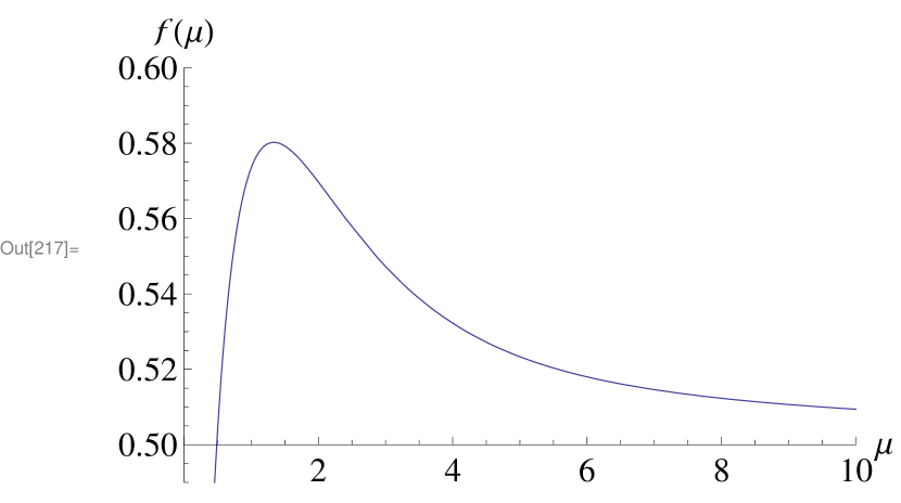
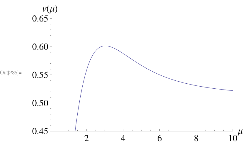
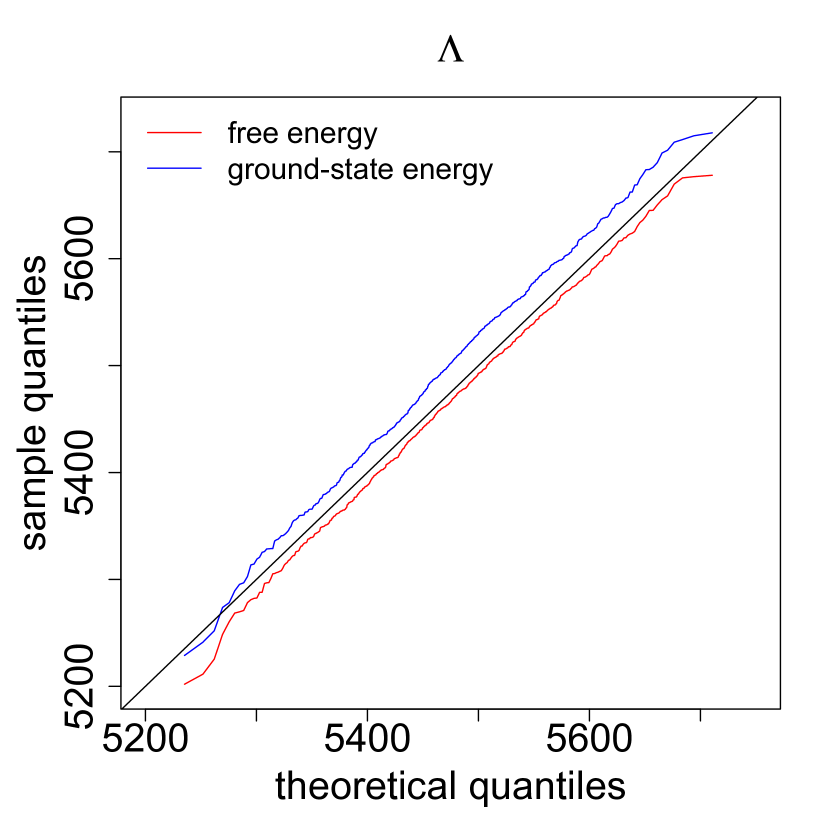
Figure 3 shows that, for networks simulated from the stochastic block model, the mean and variance of $\Lambda$ are very well fit by our formulas. We have not attempted to compute higher moments of $\Lambda$. However, if we assume that $D_{u}$ are independent, then the simplest form of the central limit theorem applies, and $n^{-1}\Lambda$ will approach a Gaussian distribution as $n\to\infty$. Quantile plots from the same simulations (Fig. 3(c)) show that a Gaussian with mean and variance from (14) and (16) is indeed a good fit. Moreover, the free energy difference and the ground state energy difference have similar distributions, as implied by our assumption that both Gibbs distributions are concentrated around the ground state. Interestingly, in Fig. 3(c), the degree is low enough that this concentration must be imperfect, but our theory still holds remarkably well. For ease of illustration, we assume that $\gamma_{r}=1/k$ and $\mu_{r}$ are the same for all $r$.

(a) $n^{-1}E\!\left(\Lambda\right)$

(b) $n^{-1}\mathrm{var}\!\left(\Lambda\right)$

(c) QQ plots for the distribution of $\Lambda$.

Figure 3: Comparison of asymptotic theory to finite-$n$ simulations. We generated networks from the stochastic block model with varying mean degree $\mu$ ($n={10}^{4}$, $k=2$, $\gamma_{1}=\gamma_{2}=1/2$, $\omega_{11}=\omega_{22}$, and $\omega_{12}/\omega_{11}=\omega_{21}/\omega_{22}=0.15$) and computed $\Lambda$ for each graph. Figures 3(a) and 3(b) show $n^{-1}E\!\left(\Lambda\right)$ and $n^{-1}\mathrm{var}\!\left(\Lambda\right)$, comparing 95% bootstrap confidence intervals (over ${10}^{3}$ replicates) to the asymptotic formulas (respectively $f(\mu)$ from (15) and $v(\mu)$ from (17)). Figure 3(c) compares the distribution of $\Lambda$ from ${10}^{4}$ replicates, all with $\mu=3$, to a Gaussian with the theoretical mean and variance. (Observe that the free energy difference and the ground state energy difference have similar distributions.)

Fundamentally, $\Lambda$ does not follow the usual $\chi^{2}$ distribution because the $\theta$ parameters are in a high-dimensional regime. For each $\theta_{u}$, we really have only one relevant observation, the node degree $D_{u}$. If $\theta_{u}$ is large, then the Poisson distribution of $D_{u}$ is well-approximated by a Gaussian, as is the sampling distribution of $\theta_{u}$’s maximum likelihood estimate, so that the usual $\chi^{2}$ analysis applies. In a sparse graph, however, all the Poisson distributions have small expected values and are highly non-Gaussian, as are the maximum likelihood estimates (Zhu et al., 2012). Said differently, the degree-corrected model has $O(n)$ more parameters than the null model. In the dense-graph case, there are $O(n^{2})$ observations, at least $O(n)$ of which are informative about each of these extra parameters. For sparse graphs, however, there are really only $O(n)$ observations, and only $O(1)$ of them are informative about each $\theta_{u}$, so the ordinary large-$n$ asymptotics cannot apply to them. As we have seen, the expected increase in likelihood from adding the $\theta$ parameters is larger than $\chi^{2}$ theory predicts, as are the fluctuations in this increase in likelihood.

This reasoning elaborates on a point made long ago by Fienberg & Wasserman (1981b) regarding hypothesis testing in the $p_{1}$ model, where each node has two node-specific parameters (for in- and out- degree); our calculations of $f(\mu)$ and $v(\mu)$ above, and especially of how and why they differ from $1/2$, go some way towards meeting Fienberg and Wasserman’s call for appropriate asymptotics for large-but-sparse graphs.

Figure 4: The network size $n$, as a function of the average degree $\mu$, above which a $\chi^{2}$ test with a nominal type I error rate of $0.05$ has an actual type I error rate $\geq 0.95$. Here we assume the asymptotic analysis of (14)–(17) for the mean and variance of the likelihood ratio.

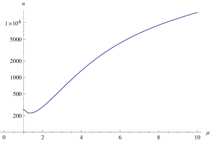
Ignoring these phenomena and using a $\chi^{2}$ test inflates the type I error rate ($\alpha$), eventually rejecting the stochastic block model for almost all graphs which it generates. Indeed, since the $\chi^{2}$ distribution is tightly peaked around $0.5n$, this inflation of $\alpha$ gets worse as $n$ gets bigger. For instance, when $\mu=5$, a $\chi^{2}$ test with nominal $\alpha=0.05$ passes has a true $\alpha\geq 0.95$ once $n\approx 3000$, while for $\mu=3$, this happens once $n\approx 700$ (Fig. 4). In essence, the $\chi^{2}$ test underestimates the amount of degree inhomogeneity we would get simply from noise, incorrectly concluding that the inhomogeneity must come from underlying properties of the nodes.

5 Results on real networks

We have derived the theoretical null distribution of $\Lambda$, and backed up our calculations with simulations. We now apply our theory to two examples, considering networks studied in Karrer & Newman (2011).

The first is a social network consisting of $34$ members of a karate club, where undirected edges represent friendships (Zachary, 1977). The network is made up of two assortative blocks, each with one high-degree hub (respectively the instructor and the club president) and many low-degree peripheral nodes. Karrer & Newman (2011) compared the performance of the ordinary and the degree-corrected block models on this network, and heavily favored degree correction, because the former leads to division into communities agreeing with ethnographic observations.

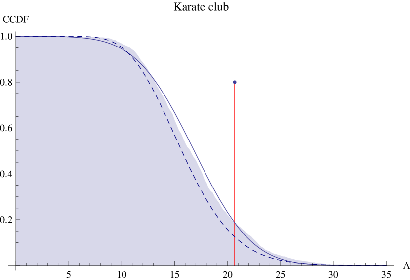
While a classic data set for network modeling, the karate club has both low degree and very small $n$. If we nonetheless use parametric bootstrapping to find the null distribution of $\Lambda$, we see that it fits a Gaussian with our predicted mean and variance reasonably well (Fig. 5(a)). The observed $\Lambda=20.7$ has a $p$-value of $0.187$ according to the bootstrap, and $0.186$ according to our Gaussian asymptotics. Thus a prudent analyst would think twice before embracing the $n$ additional degree-correction parameters. Indeed, using active learning, Moore et al. (2011) found that the stochastic block model labels most of the nodes correctly if the instructor and president are forced into different blocks. This implies that the degree inhomogeneity is mild, and that only a handful of nodes are responsible for the better performance of the degree-corrected model.

Note that if we apply standard $\chi^{2}$ testing to the karate club, we obtain a lower $p$-value of $0.125$. As in Fig. 4, $\chi^{2}$ testing underestimates the extent to which an inhomogeneous degree distribution can result simply from noise, causing it to reject the null model more confidently than it should.

Figure 5: Hypothesis testing with real networks; both panels show the complementary cumulative distribution function of the log-likelihood ratio $\Lambda$ for testing for degree correction. (a): Zachary’s karate club (Zachary, 1977) ($n=34$). The distribution found by parametric bootstrapping (shaded) fits reasonably well to a Gaussian (curve) with our theoretical mean and variance. The observed $\Lambda=20.7$ (marked with the red line) has $p$-values of $0.186$ and $0.187$ according to the bootstrap and theoretical distributions respectively, whereas the $\chi^{2}$ test (dashed) has a $p$-value of $0.125$. (b): A network of political blogs (Adamic & Glance, 2005) ($n=1222$). The bootstrap distribution (shaded) is very well fit by our theoretical Gaussian (curve) as well as the $\chi^{2}$ test (dashed). The actual log-likelihood ratio is so far in the tail that its $p$-value is effectively zero (see inset). Thus for the blog network, we can decisively reject the ordinary block model in favor of the degree-corrected model, while for the karate club, the evidence is less clear.

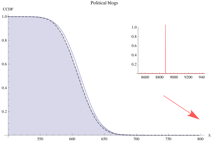
The second example is a network of political blogs in the US assembled by Adamic & Glance (2005). As in Karrer & Newman (2011), we focus on the giant component, which contains $1222$ blogs with $19087$ links between them. The blogs have known political leanings, and were labeled as either liberal or conservative. The network is politically assortative, with highly right-skewed degree distributions within each block, so degree correction greatly assists in recovering political divisions, as observed by Karrer & Newman (2011). This time around, our hypothesis testing procedure completely agrees with their choice of model. As shown in Fig. 5(b), the bootstrap distribution of $\Lambda$ is very well fit by a Gaussian with our theoretical prediction of the mean and variance. The observed log-likelihood ratio $\Lambda=8883$ is $330$ standard deviations above the mean. It is essentially impossible to produce such extreme results through mere fluctuations under the null model. Thus, for this network, introducing $n$ extra parameters to capture the degree heterogeneity is fully justified.

The blog network shows several advantages of our theoretical approach over just using bootstrapping. As with many other real networks, $n$ is large enough that bootstrapping is quite slow, but for the same reason the Gaussian approximation for $\Lambda$ is fairly tight.

6 Conclusion

Deciding between ordinary and degree-corrected stochastic block models for sparse graphs presents a difficult hypothesis testing problem. The distribution of the log-likelihood ratio $\Lambda$ does not follow the classic $\chi^{2}$ theory, because the nuisance parameter $\theta$, only present in the alternative, is in a high-dimensional regime. We have nonetheless derived $\Lambda$’s mean and variance in the limit of large, sparse graphs, where node degrees become independent and Poisson. Simulations confirm the accuracy of our theory for moderate $n$, and we applied it to two real networks.

Beyond hypothesis testing, two standard approaches to model selection are information criteria and cross-validation. While we have not directly dealt with the former, the derivations of such popular criteria as AIC or DIC use exactly the same asymptotics as the $\chi^{2}$ test (Claeskens & Hjort, 2008, ch. 2); these tools will break down for the same reasons $\chi^{2}$ theory fails. As for cross-validation, standard practice in machine learning suggests using multi-fold cross-validation, but the global dependence of network data means there is (as yet) no good way to split a graph into training and testing sets. Predicting missing links or tagging false positives are popular forms of leave-$k$-out cross-validation in the network literature (Clauset et al., 2008; Guimera & Sales-Pardo, 2009), but leave-$k$-out does not converge on the true model even for independent and identically-distributed data (Claeskens & Hjort, 2008, §2.9). Thus, while our results apply directly only to the specific problem of testing the need for degree correction, they open the way to more general approaches to model selection and hypothesis testing in a wide range of network problems.

Appendix A Behavior of $\Lambda$ under the null hypothesis

For simplicity we focus on one block with expected degree $\mu$. Independence between blocks will then recover the expressions (14) and (16) where the mean and variance of $\Lambda$ is a weighted sum over blocks. We have

$$\Lambda=\sum_{i=1}^{n}{D_{i}\log{\frac{D_{i}}{\overline{D}}}}=\sum_{i}{D_{i}\log{D_{i}}}-\left(\sum_{i}{D_{i}}\right)\log{\left(\sum_{i}{D_{i}}\right)}+\left(\sum_{i}{D_{i}}\right)\log{n},$$ (18)

where $\overline{D}=(1/n)\sum_{i}{D_{i}}$ is the empirical mean degree. We wish to compute the mean and expectation of $\Lambda$ if the data is generated by the null model.

If $D\sim\text{Poi}(\mu)$, let $f(\mu)$ denote the difference between the expectation of $D\log{D}$ and its most probable value $\mu\log{\mu}$:

$$f(\mu)=\left(\sum_{d=1}^{\infty}\frac{e^{-\mu}\mu^{d}}{d!}d\log{d}\right)-\mu\log\mu.$$ (19)

Assume that the $D_{i}$ are independent and $\sim\text{Poi}(\mu)$; this is reasonable in a large sparse graph, since the correlations between degrees of different nodes is $O(1/n)$. Then $n\overline{D}\sim\text{Poi}(n\mu)$, and (18) gives

$$E\!\left(\Lambda\right)=nf(\mu)-f(n\mu).$$ (20)

To grasp what this implies, begin by observing that $f(\mu)$ converges to $1/2$ when $\mu$ is large. Thus in the limit of large $n$, $E\!\left(\Lambda\right)=nf(\mu)-\frac{1}{2}$. When $\mu$ is large, this gives $E\!\left(\Lambda\right)=(n-1)/2$, just as $\chi^{2}$ theory suggests. However, as Fig. 2 shows, $f(\mu)$ deviates noticeably from $1/2$ for finite $\mu$. We can obtain the leading corrections as a power series in $1/\mu$ by approximating (19) with the Taylor series of $d\log d$ around $d=\mu$, giving

$$f(\mu)=\frac{1}{2}+\frac{1}{12\mu}+\frac{1}{12\mu^{2}}+O(1/\mu^{3}).$$

Computing the variance is harder. It will be convenient to define several functions. If $D\sim\text{Poi}(\mu)$, let $\phi(\mu)$ denote the variance of $D\log{D}$:

$$\phi(\mu)=\mathrm{var}\!\left(D\log{D}\right)=\sum_{d=0}^{\infty}\frac{e^{-\mu}\mu^{d}}{d!}(d\log d)^{2}-\left(f(\mu)+\mu\log{\mu}\right)^{2}.$$ (21)

We will also use

$$c(\mu)=\mathrm{cov}\!\left(D,D\log{D}\right)=\sum_{d=1}^{\infty}\frac{e^{-\mu}\mu^{d}}{d!}d^{2}\log d-\mu\left(f(\mu)+\mu\log\mu\right).$$ (22)

Finally, let $\psi\geq\mu$, and let $D$ and $U$ be independent and Poisson with mean $\mu$ and $\psi-\mu$ respectively. Then let

$$r(\mu,\psi) = \mathrm{cov}\!\left(D\log D,(D+U)\log(D+U)\right)$$ (23)

$$= E\!\left((D\log D)((D+U)\log(D+U))\right)-E\!\left(D\log D\right)E\!\left((D+U)\log(D+U)\right)$$

$$= E\!\left((D\log D)((D+U)\log(D+U))\right)-\left(f(\mu)+\mu\log\mu\right)\left(f(\psi)+\psi\log{\psi}\right),$$

where we used the fact that $D+U\sim\text{Poi}(\psi)$.

Again assuming that the $D_{i}$ are independent, we have the following terms and cross-terms for the variance of (18) :

$$\mathrm{var}\!\left(\sum_{i}{D_{i}\log{D_{i}}}\right) =n\phi(\mu)$$

$$\mathrm{var}\!\left(\left(n\overline{D}\right)\log{\left(n\overline{D}\right)}\right) =\phi(n\mu)$$

$$\mathrm{var}\!\left(n\overline{D}\right) =n\mu$$

$$\mathrm{cov}\!\left(\sum_{i}{D_{i}\log{D_{i}}},\left(n\overline{D}\right)\log{\left(n\overline{D}\right)}\right) =nr(\mu,n\mu)$$

$$\mathrm{cov}\!\left(\sum_{i}{D_{i}\log{D_{i}}},n\overline{D}\right) =nc(\mu)$$

$$\mathrm{cov}\!\left(\left(n\overline{D}\right)\log{n\overline{D}},n\overline{D}\right) =c(n\mu)$$

Putting this all together, we have

$$\mathrm{var}\!\left(\Lambda\right)=n\phi(\mu)+\phi(n\mu)+n\mu\log^{2}{n}-2nr(\mu,n\mu)+2\left(nc(\mu)-c(n\mu)\right)\log{n}.$$ (24)

For large $\mu$, Taylor-expanding the summands of (21) and (22) yields

$$\phi(\mu) =\mu\log^{2}{\mu}+2\mu\log{\mu}+\mu+\frac{1}{2}+O\left(\frac{\log\mu}{\mu}\right)$$

$$c(\mu) =\mu\log{\mu}+\mu+O(1/\mu).$$

Also, when $\psi\gg\mu$ and $\mu=O(1)$, using $\log{(D+U)}\approx\log U+D/U$ lets us simplify (23), giving

$$r(\mu,\lambda) =E\!\left(D^{2}\log{D}\right)(1+\log\lambda)$$

$$+E\!\left(D\log{D}\right)E\!\left(U\log U\right)$$

$$-E\!\left(D\log{D}\right)E\!\left((D+U)\log{D+U}\right))+O(1/\lambda).$$

In particular, setting $\psi=n\mu$ gives

$$r(\mu,n\mu)=c(\mu)(1+\log n\mu)+O(1/n).$$

Finally, keeping $O(n)$ terms in (24) and defining $v(\mu)$ as in (16) gives

$$v(\mu)=\lim_{n\to\infty}\frac{1}{n}\mathrm{var}\!\left(\Lambda\right)=\phi(\mu)+\mu(1+\log\mu)^{2}-2c(\mu)(1+\log\mu).$$ (25)

Using the definitions of $\phi$ and $c$, we can write this more explicitly as

$$v(\mu)=\mu(1+\log\mu)^{2}+\mathrm{var}\!\left(D\log{D}\right)-2(1+\log\mu)\mathrm{cov}\!\left(D,D\log{D}\right),$$ (26)

where $D\sim\text{Poi}(\mu)$. We plot this function in Fig. 2(b). It converges to $1/2$ in the limit of large $\mu$, but it is significantly larger for finite $\mu$.

References

- Adamic & Glance (2005) Adamic, L. A. & Glance, N. (2005). The political blogosphere and the 2004 US election: Divided they blog. In Proceedings of the 3rd International Workshop on Link Discovery [LinkKDD ’05], J. Adibi, M. Grobelnik, D. Mladenic & P. Pantel, eds. New York: ACM.
- Airoldi et al. (2008) Airoldi, E. M., Blei, D. M., Fienberg, S. E. & Xing, E. P. (2008). Mixed membership stochastic blockmodels. Journal of Machine Learning Research 9, 1981–2014.
- Allesina & Pascual (2009) Allesina, S. & Pascual, M. (2009). Food web models: a plea for groups. Ecology letters 12, 652–662.
- Beal & Ghahramani (2006) Beal, M. J. & Ghahramani, Z. (2006). Variational Bayesian learning of directed graphical models with hidden variables. Bayesian Analysis 1, 7983–832.
- Bickel & Chen (2009) Bickel, P. J. & Chen, A. (2009). A nonparametric view of network models and Newman-Girvan and other modularities. Proceedings of the National Academy of Sciences (USA) 106, 21068–21073.
- Chung & Lu (2002) Chung, F. & Lu, L. (2002). Connected components in random graphs with given expected degree sequences. Annals of Combinatorics 6, 125–145.
- Claeskens & Hjort (2008) Claeskens, G. & Hjort, N. L. (2008). Model Selection and Model Averaging. Cambridge, England: Cambridge University Press.
- Clauset et al. (2008) Clauset, A., Moore, C. & Newman, M. E. J. (2008). Hierarchical structure and the prediction of missing links in networks. Nature 453, 98–101.
- Davison & Hinkley (1997) Davison, A. C. & Hinkley, D. V. (1997). Bootstrap Methods and their Applications. Cambridge, England: Cambridge University Press.
- Decelle et al. (2011a) Decelle, A., Krzakala, F., Moore, C. & Zdeborová, L. (2011a). Asymptotic analysis of the stochastic block model for modular networks and its algorithmic applications. Physical Review E 84, 066106.
- Decelle et al. (2011b) Decelle, A., Krzakala, F., Moore, C. & Zdeborová, L. (2011b). Inference and phase transitions in the detection of modules in sparse networks. Physical Review Letters 107, 065701.
- Dempster et al. (1977) Dempster, A. P., Laird, N. M. & Rubin, D. B. (1977). Maximum likelihood from incomplete data via the EM algorithm. Journal of the Royal Statistical Society B 39, 1–38.
- Fienberg & Wasserman (1981a) Fienberg, S. E. & Wasserman, S. (1981a). Categorical data analysis of single sociometric relations. In Sociological Methodology 1981, S. Leinhardt, ed. San Francisco: Jossey-Bass, pp. 156–192.
- Fienberg & Wasserman (1981b) Fienberg, S. E. & Wasserman, S. (1981b). An exponential family of probability distributions for directed graphs: Comment. Journal of the American Statistical Association, 76, 54–57.
- Geyer (2005) Geyer, C. J. (2005). Le Cam made simple: Asymptotics of maximum likelihood without the LLN or CLT or sample size going to infinity. Tech. Rep. 643, School of Statistics, University of Minnesota.
- Guimera & Sales-Pardo (2009) Guimera, R. & Sales-Pardo, M. (2009). Missing and spurious interactions and the reconstruction of complex networks. Proceedings of the National Academy of Sciences (USA) 106, 22073–22078.
- Holland et al. (1983) Holland, P. W., Laskey, K. B. & Leinhardt, S. (1983). Stochastic blockmodels: First steps. Social Networks 5, 109–137.
- Holland & Leinhardt (1981) Holland, P. W. & Leinhardt, S. (1981). An exponential family of probability distributions for directed graphs. Journal of the American Statistical Association 76, 33–50.
- Hunter & Handcock (2006) Hunter, D. R. & Handcock, M. S. (2006). Inference in curved exponential family models for networks. Journal of Computational and Graphical Statistics 15, 565–583.
- Karrer & Newman (2011) Karrer, B. & Newman, M. E. J. (2011). Stochastic blockmodels and community structure in networks. Physical Review E 83, 016107.
- Moore et al. (2011) Moore, C., Yan, X., Zhu, Y., Rouquier, J.-B. & Lane, T. (2011). Active learning for node classification in assortative and disassortative networks. In 17th ACM SIGKDD Conference on Knowledge Discovery and Data Mining [KDD 2011], C. Apte, J. Ghosh & P. Smyth, eds.
- Mørup & Hansen (2009) Mørup, M. & Hansen, L. K. (2009). Learning latent structure in complex networks. In NIPS Workshop on Analyzing Networks and Learning with Graphs, E. Airoldi, J. Kleinberg, J. Leskovec & J. Tenenbaum, eds.
- Mossel et al. (2012) Mossel, E., Neeman, J. & Sly, A. (2012). Stochastic block models and reconstruction. arxiv.org.
- Neal & Hinton (1998) Neal, R. M. & Hinton, G. E. (1998). A view of the EM algorithm that justifies incremental, sparse, and other variants. In Learning in Graphical Models, M. I. Jordan, ed. Dordrecht: Kluwer Academic.
- Newman (2002) Newman, M. E. J. (2002). Assortative mixing in networks. Physical Review Letters 89, 208701.
- Newman (2003) Newman, M. E. J. (2003). Mixing patterns in networks. Physical Review E 67, 026126.
- Perry & Wolfe (2012) Perry, P. O. & Wolfe, P. J. (2012). Null models for network data. E-print, arxiv:1201.5871.
- Porter et al. (2009) Porter, M. A., Onnela, J.-P. & Mucha, P. J. (2009). Communities in networks. Notices of the American Mathematical Society 56, 1082–1097 and 1164–1166.
- Reichardt et al. (2011) Reichardt, J., Alamino, R. & Saad, D. (2011). The interplay between microscopic and mesoscopic structures in complex networks. PLoS ONE 6, e21282.
- Rinaldo et al. (2011) Rinaldo, A., Petrović, S. & Fienberg, S. E. (2011). Maximum likelihood estimation in the beta model. arxiv.org.
- Schervish (1995) Schervish, M. J. (1995). Theory of Statistics. Berlin: Springer-Verlag.
- Snijders & Nowicki (1997) Snijders, T. A. B. & Nowicki, K. (1997). Estimation and prediction for stochastic blockmodels for graphs with latent block structure. Journal of Classification 14, 75–100.
- Wasserman & Anderson (1987) Wasserman, S. & Anderson, C. (1987). Stochastic a posteriori blockmodels: Construction and assessment. Social Networks 9, 1–36.
- Yedidia et al. (2003) Yedidia, J. S., Freeman, W. T. & Weiss, Y. (2003). Understanding belief propagation and its generalizations. In Exploring Artificial Intelligence in the New Millennium [IJCAI 2001], G. Lakemeyer & B. Nebel, eds. San Francisco: Morgan Kaufmann.
- Yedidia et al. (2005) Yedidia, J. S., Freeman, W. T. & Weiss, Y. (2005). Constructing free-energy approximations and generalized belief propagation algorithms. IEEE Transactions on Information Theory 51, 2282–2312.
- Zachary (1977) Zachary, W. W. (1977). An information flow model for conflict and fission in small groups. Journal of Anthropological Research 33, 452–473.
- Zhu et al. (2012) Zhu, Y., Yan, X. & Moore, C. (2012). Generating and inferring communities with inhomogeneous degree distributions. Eprint, arxiv:1205.7009.