Optimized Wang-Landau sampling of lattice polymers: Ground state search and folding thermodynamics of HP model proteins

Abstract

Coarse-grained (lattice-) models have a long tradition in aiding efforts to decipher the physical or biological complexity of proteins. Despite the simplicity of these models, however, numerical simulations are often computationally very demanding and the quest for efficient algorithms is as old as the models themselves. Expanding on our previous work [T. Wüst and D. P. Landau, Phys. Rev. Lett. 102, 178101 (2009)], we present a complete picture of a Monte Carlo method based on Wang-Landau sampling in combination with efficient trial moves (pull, bond-rebridging and pivot moves) which is particularly suited to the study of models such as the hydrophobic-polar (HP) lattice model of protein folding. With this generic and fully blind Monte Carlo procedure, all currently known putative ground states for the most difficult benchmark HP sequences could be found. For most sequences we could also determine the entire energy density of states and, together with suitably designed structural observables, explore the thermodynamics and intricate folding behavior in the virtually inaccessible low-temperature regime. We analyze the differences between random and protein-like heteropolymers for sequence lengths up to 500 residues. Our approach is powerful both in terms of robustness and speed, yet flexible and simple enough for the study of many related problems in protein folding.

I Introduction

Coarse-grained (lattice-) models play an important role in clarifying questions of generic understanding in protein folding and protein structure prediction.dill:protein_sci:99 ; kolinski:polymer:04 With the aim of separating relevant features from unimportant details, such “minimalist” models allow us to capture only those forces that effectively drive a system and thus to eventually find the “basic laws” behind a particular phenomenon. Arguably one of the simplest protein models is the hydrophobic-polar (HP) lattice model introduced by Dill et al.dill:biochemistry:85 ; *lau:macromolecules:89 Classifying the 20 amino acids in just two types (hydrophobic and polar), the HP model contains only two physical ingredients: an excluded volume effect (self-avoiding walk on a lattice) and an effective monomer-monomer interaction among non-bonded nearest neighbor H monomers, mimicking the hydrophobic interaction which is considered a main driving force of protein folding. Owing to the HP and similar models, many fundamental concepts and questions, e. g. the relationship between protein sequence and structure, the notions of energy landscapes and folding funnels, thermodynamic transitions towards and stability of the native state, or the kinetic mechanisms of folding, could be systematically investigated by means of computer simulations.sali:nature:94 ; shakhnovich:curr_opin_struct_biol:97 ; dill:protein_sci:99

Minimalist protein models also laid a basis for the study of many related problems of biological interest. Examples include protein aggregation (multi-chain systems),cellmer:pnas:05 ; *zhang:biophys_chem:08 surface adsorption,castells:phys_rev_E:02 ; *bachmann:phys_rev_E:06; radhakrishna:j_chem_phys:12 protein folding in heterogeneous (e. g. membranes)gersappe:j_chem_phys:93 ; *bonaccini:phys_rev_E:99; *zhdanov:proteins:01 and crowded or confined environments,ping:j_chem_phys:03 or the formation of knots in proteins.faisca:phys_biol:10

A common requirement for such studies is a generic Monte Carlo method capable of efficiently sampling the conformational spaces of the system. Despite the formal simplicity and minimalistic framework of the HP and related models, however, numerical simulations are often computationally very demanding. The reliable numerical estimation of the low temperature ($T$) thermodynamic behavior of these models is particularly challenging. The origin of this difficulty is twofold: (i) Steric constraints imposed by the underlying lattice (attrition problem) and other conformational or energy barriers lead to rough energy landscapes and, thus, hamper the proper sampling of conformational space. These issues become particularly noticeable at low $T$, where the polymers exhibit very compact conformations. (ii) The low-energy conformations often have a very low degeneracy and the energy density of states (DOS), $g(E)$, (which measures energy degeneracy) increases rapidly with chain length or number of energy levels.

Whereas problem (i) is not unique to protein-like models and also appears in simulations of (off-) lattice homopolymers,rampf:j_polym_sci_B_polym_phys:06 ; *seaton:phys_rev_E:10 problem (ii) is a direct consequence of protein sequence specificity. For example, the HP sequence with 103 monomers (investigated below) has 59 energy levels and $g(E)$ spans more than 50 orders of magnitude, whereas the corresponding interacting self-avoiding walk (i. e. homopolymer of the same length with H monomers only) contains 139 energies but with a $g(E)$ range of 38 orders of magnitude only.

Together, these obstacles pose a significant challenge to numerical studies and have led to the invention of various sophisticated, but often also specialized algorithms, such as sequential importance samplingzhang:j_chem_phys:02 and chain-growth methods,otoole:j_chem_phys:92 ; beutler:protein_sci:96 the most prominent example being the pruned-enriched Rosenbluth method (PERM)grassberger:phys_rev_E:97 and its variantsfrauenkron:phys_rev_lett:98 ; *bastolla:proteins:98; hsu:j_chem_phys:03 ; *hsu:phys_rev_E:03 and flat-histogram/multicanonical versions,prellberg:phys_rev_lett:04 ; bachmann:phys_rev_lett:03 ; *bachmann:j_chem_phys:04 equi-energy sampling,kou:j_chem_phys:06 multi-self overlap ensemble Monte Carlo,iba:j_phys_soc_jpn:98 ; *chikenji:phys_rev_lett:99 fragment regrowth Monte Carlo,zhang:j_chem_phys:07 etc. (see also references therein).

Since finding the lowest energy conformation(s) for a given HP sequence is an NP-complete problem,berger:j_comput_biol:98 ; *crescenzi:j_comput_biol:98 the model has also raised interest in the computer science community as a challenge in combinatorial optimization. Targeted specifically to the search of minimal energy conformations, several (heuristic) algorithms have been proposed, ranging from genetic algorithmsunger:j_mol_biol:93 ; konig:biosystems:99 and evolutionary Monte Carloliang:j_chem_phys:01 or ant colony modelsshmygelska:bmc_bioinformatics:05 to constraint-based algorithms.backofen:constraints:06 However, we stress that such approaches, while potentially advancing research in protein structure prediction, are only of limited use to the understanding of the thermodynamics/kinetics of protein folding.

One motivation behind this work was the desire to develop an algorithm with the power to attack the HP model and the flexibility to be applicable also to more general setups as described above. Expanding on previous work,wuest:comput_phys_commun:08 ; *wuest:phys_rev_lett:09 we present here a generic, fully blind and fast Monte Carlo procedure, based on the combination of Wang-Landau samplingwang:phys_rev_lett:01 ; *wang:phys_rev_E:01 with efficient Monte Carlo trial moves, which is very successful both in finding low energy conformations and obtaining thermodynamic properties for HP-like models over the entire temperature range, including the difficult to access low-temperature regime. Wang-Landau sampling has been shown to be very efficient and robust in various fields of statistical physics including simulations of spin systems,zhou:phys_rev_lett:06 ; torbrugge:phys_rev_B:07 polymers and proteins,rampf:j_polym_sci_B_polym_phys:06 ; *seaton:phys_rev_E:10; gervais:j_chem_phys:09 or even numerical integration,troster:phys_rev_E:05 ; li:comput_phys_commun:07 (see also references therein). Instead of sampling a system at a single temperature, one estimates $g(E)$ from which thermodynamic quantities at any temperature can be derived. By performing a random walk in energy space, the algorithm is well suited for overcoming energy barriers typically encountered in complex free energy landscapes. However, in order to fully exploit the capabilities of the algorithm for systems which also have complex conformational spaces, suitably chosen Monte Carlo trial moves must be introduced. Finding an optimal interplay between Monte Carlo driver, trial move set and efficient implementation is a significant achievement of the present study.

The paper is organized as follows: We first provide a detailed account of our methodology (Sec. II). Comparing with two other successful methods, we then demonstrate its efficiency in finding low energy states for common benchmark HP sequences (Sec. III.1). In Sec. III.2 we study the thermodynamics of these model proteins and show how to elucidate the subtle conformational changes occurring at low temperature by means of suitable structural observables. In Sec. III.3, we investigate the generic differences in the thermodynamic behavior between random and protein-like heteropolymers for long chain lengths. Finally, in Sec. IV gives our conclusion.

II Model and Simulation Method

HP model proteins consist of isolated self-avoiding walks (SAWs) on a regular lattice with each site of the walk being occupied by a monomer (either polar or hydrophobic). Here, we only consider the commonly studied square (2D) and simple cubic (3D) lattices. Self-avoidance means that no lattice site can be occupied by more than one monomer at any time. $N$ denotes the number of monomers (i. e. the SAW has length $N-1$). The energy $E$ of a protein conformation is defined by the number of non-bonded nearest neighbor contacts among hydrophobic monomers, each of which being associated with an attractive energy $-\epsilon$.

In the canonical ensemble the partition function is

$$Z_{N}(T)=\sum_{\omega\in\Omega_{N}}e^{-E/kT}=\sum_{E}g(E)e^{-E/kT},$$ (1)

where $k$ is Boltzmann’s constant and $T$ is the temperature. The first sum runs over the set of all conformations $\Omega_{N}$ while the second sum over all energies $E$ introduces the energy density of states, $g(E)$. Since $g(E)$ does not depend on $T$, the second form allows us to calculate $Z_{N}(T)$ at any $T$ and is thus the target quantity of our interest.

Despite the conceptual simplicity of the model, estimating $g(E)$ over the entire - and in particular low - energy range of long HP protein sequences is a non-trivial task (see the Introduction). Principally, it can be subdivided into three aspects: (A) choice of Monte Carlo sampling scheme (Monte Carlo driver); (B) choice of appropriate and efficient Monte Carlo trial moves; (C) efficient and fast implementation.

II.1 Wang-Landau sampling

In Wang-Landau sampling, the a priori unknown density of states $g(E)$ of energy $E$ is iteratively determined by performing a random walk in energy space seeking to sample a flat energy distribution. The expression “random walk in energy space” emanates from the fact that conformations are sampled with a probability approaching $\sim 1/g(E)$ resulting in a uniform distribution in $E$. Note that the method can, in principle, be applied to any type of observable (not only energy) or to several observables simultaneously.zhou:phys_rev_lett:06 ; torbrugge:phys_rev_B:07

Initially, $g(E)=1,\forall E$. A Monte Carlo trial move from a state (or conformation) $A$ with energy $E_{A}$ to a state $B$ with energy $E_{B}$ is accepted according to the transition probability

$$P(A\rightarrow B)=\min\left(1,\frac{g(E_{A})}{g(E_{B})}\right).$$ (2)

After each trial move, $g$ is modified as $g(E_{t})=f\times g(E_{t})$ ($f>1$ is called the modification factor, initially $f=e^{1}$) and, simultaneously, a histogram $H$ is updated, $H(E_{t})=H(E_{t})+1$, where $t$ stands for state $B$ if the trial move has been accepted, otherwise $t\equiv A$. Once the energy distribution in $H$ is sufficiently flat (i. e. $H(E)\geq p\langle H(E)\rangle$ for all energies $E$, where $\langle H(E)\rangle$ is the average histogram and $0<p<1$ is called the “flatness criterion”), the modification factor $f$ is reduced as $f=\sqrt{f}$, $H$ is reset to zero and a new iteration begins. This process is repeated until $f$ falls below a threshold ($f_{\text{final}}\approx 1$) at which point $g(E)$ has converged towards the correct density of states.

The accuracy of the calculated $g(E)$ is controlled by two simulation parameters: the final modification factor $f_{\text{final}}$ and the flatness criterion $p$. For a discussion on the choice of these parameters, see below.

Knowledge of the upper and lower energy boundaries as well as any nonexistent energy states (energy gaps) within this range, is essential in the WL algorithm in order to examine the flatness of the histogram and, ultimately, to control the course of the simulation. Often, however, the exact energy range is a priori unknown, (hence the use of ground state search algorithms, e. g. for the HP model). To solve this dilemma, performing a pre-WL run to determine the energy range and thereafter fix the sampling to this range has been proposed.troster:phys_rev_E:05 ; torbrugge:phys_rev_B:07 The problem with such an approach is two-fold: (i) The pre-WL run may take a long time to accurately explore energy space and it is thus unclear when to stop. (ii) Often, new energy states are found rather late in the course of the simulation when the running DOS estimate has resulted in a sufficiently “flat sampling”.

To overcome these difficulties, the following procedure proved to be most efficient:wuest:comput_phys_commun:08 ; *wuest:phys_rev_lett:09 Every time a new energy state $E_{\text{new}}$ is found, it is marked as “visited”, $g(E_{\text{new}})$ is set to $g_{\text{min}}$ (i. e. the minimum of $g$ among all previously visited energy states) and the histogram is reset to zero. The flatness of the histogram is always checked among visited energy states only, with a sufficiently long interval between subsequent checks (e. g. every $10^{6}$ MC moves). With this self-adaptive procedure, new regions of conformation space can be explored while the current estimate of the DOS is further refined which, in turn, tends to improved sampling (with respect to a flat histogram in energy space).

II.2 Monte Carlo trial moves

Compared to traditional Monte Carlo schemes, the Wang-Landau algorithm has been an enormous improvement in overcoming the obstacles typically encountered near phase transitions. However, the advantageous dynamics of this Monte Carlo driver is most effective when used in concert with suitable Monte Carlo trial moves.

Usually, studies of lattice polymers introduce local moves that change a single bond (end flips), two bonds (corner flips) or three bonds (crankshafts).sokal:95 However, such moves suffer from slow dynamics and are non-ergodic.madras:j_stat_phys:87 Global moves, like pivot operations, sample conformational space of (athermal) self-avoiding walks very efficientlymadras:j_stat_phys:88 but in the low temperature, compact, polymer phase their acceptance ratio becomes negligible.

The key to our approach is the combination of two “non-traditional” Monte Carlo trial moves which complement one another extremely well, namely pull moveslesh:recomb:03 and bond-rebridging moves,deutsch:j_chem_phys:97 see Fig. 1.

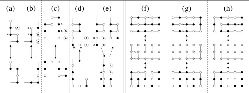
Figure 1: Illustration of MC trial moves. Left panel: Pull moves: (a) single-bead move (kink flip); (b) two-beads move; (c) internal multi-beads move; (d) chain-terminal move; (e) chain-terminal move forming a “hook”; this move is not allowed (non-reversible). The dotted circles denote the primary (A) and secondary (B) displacement sites of monomers A and B, respectively. Subsequent monomers are then pulled sequentially to previously occupied sites until the chain reaches a new valid configuration. Right panel: Bond-rebridging moves: (f) chain internal move (“type 1” in Ref. deutsch:j_chem_phys:97, ) with two consecutive cut-and-join steps (in the intermediate stage, the chain is divided into a circular and a linear piece); (g) chain internal move (“type 2” in Ref. deutsch:j_chem_phys:97, ) with a single cut-and-join step; (h) chain-terminal move. Bond cutting and rejoining are marked with a cross and a dashed line, respectively. Note that cutting/rejoining steps may alter the HP sequence along the chain (indicated by beads colored in gray in the intermediate stages), so once the chain has moved to a new conformation, monomer types must be relabeled to ensure the same HP sequence. Double arrows indicate reversibility of moves. All examples have been adopted from Refs. lesh:recomb:03, , kou:j_chem_phys:06, and deutsch:j_chem_phys:97, .

Pull moves: This recently introduced trial move allows for the close-fitting motion of a polymer chain within a confining environment by continuously “pulling” portions of the polymer to unoccupied neighboring sites of the chain. For a detailed description, see Ref. lesh:recomb:03, . Pull moves are reversible and ergodic. They feature a good balance between local and global conformational changes; on average, less than 10 monomers are displaced during a pull move, keeping the change in energy per move modest and thus always guaranteeing a reasonable acceptance ratio. Moreover, pull moves provide an efficient means of folding and unfolding because of their reptation-like dynamics and the fact that monomers move largely along paths that were already occupied; hence, it is less likely that a trial move violates the ”excluded volume” condition. Such features are vital in WL sampling to explore both conformation and energy space efficiently. Fig. 1 shows some examples of valid pull moves and one invalid (non-reversible) end pull move (for completeness, we note this case explicitly here since it was not clearly mentioned in the original descriptions).

Bond-rebridging moves: With decreasing temperature, polymers form dense and compact conformations leaving only very few unoccupied lattice sites in the bulk. Therefore, monomer displacing trial moves are restricted to act on surface beads, and thus become more and more ineffective with lower $T$ and larger $N$. In contrast, bond-rebridging (or connectivity altering) movespant:macromolecules:95 ; ramakrishnan:j_chem_phys:97 ; deutsch:j_chem_phys:97 allow the polymer to change its conformation even at highest densities by reordering bonds while leaving monomer positions unchanged. Moreover, they facilitate long range topological changes, e. g. entanglement, which would otherwise require very costly unfolding/folding processes. This latter feature also becomes important when the WL sampling of the DOS is split up into energy subintervals as it substantially reduces the risk of “locking-out” conformational space. Fig. 1 shows the three types of bond-rebridging moves applied here; for a detailed discussion, see Ref. deutsch:j_chem_phys:97, .

The combination of bond-rebridging and pull moves yielded an overall speed-up in WL convergence of up to a factor three as compared to pull moves only. More importantly, ground states of some HP sequences would not have been found at all without the concerted interplay of these two types of trial moves.

To further accelerate global conformational changes, we supplemented our trial move set with pivot moves.sokal:95 Although their impact is quite sequence dependent, pivot moves further improved the sampling (i. e. WL convergence time) for most of the HP sequences considered below. Pivot moves become a prerequisite for chain lengths $N\gg 100$ since the dynamics of pull moves alone would be too slow to sample the extended coil conformations of long polymers.

Detailed balance: Wang-Landau sampling is a non-Markovian process and its convergence has been shown without relying on the condition of detailed balance.zhou:phys_rev_E:05 ; zhou:phys_rev_E:08 Nonetheless, it is important that trial moves fulfill detailed balance in order to avoid systematic errors. Unlike, for instance, single-spin-flip dynamics in the Ising model, where the number of trial moves is always constant, here the number of valid trial moves may vary from one conformation to the next. It is therefore necessary to account for a possible imbalance when performing a Monte Carlo step from a starting state $A$ to a trial state $B$. One possibility to do so, is to enumerate all valid trial moves in $A$ and $B$, and augment the usual Wang-Landau (or Metropolis-Hastings) acceptance rule with a term compensating for unequal trial move ratios.kou:j_chem_phys:06 ; wuest:comput_phys_commun:08 ; *wuest:phys_rev_lett:09 This enumeration process is, however, computationally very expensive. A more efficient Monte Carlo scheme that avoids this counting procedure in the case of pull moves has been proposed in Ref. swetnam:phys_chem_chem_phys:09, Detailed balance is guaranteed if a trial move is reversible and the reverse move has the same probability of being selected as the original move. Therefore, it is possible to carry out a “trial-and-error” procedure where trial moves are chosen randomly, but with constant probability, i. e. independent of the current conformation. Whenever such a trial move is invalid (e. g. resulting in overlapping monomers) the move is rejected and $g(E),H(E)$ of the old conformation are updated. Otherwise, the move is accepted according to Eq. (2). A careful analysis shows that this procedure can be applied for all three move types used here. So do all of them fulfill reversibility; sometimes multiple possibilities exist to go from $A$ to $B$, but this number is always the same in both directions for a given type of move. Thus, it suffices to employ selection routines for each move type which ensure that trial moves are chosen with constant probability:

(i) Pull moves: a list is generated prior to simulation, specifying the relative displacements of the primary and secondary pull sites ($A$ and $B$ monomers in Fig. 1) for the entirely elongated polymer chain. This particular conformation features the maximally possible pull moves,

$$\begin{split}\max n_{\text{pull}}&=(N-2)\times 4(d-1)\\ &\quad+2\times(2d-1+(2d-2)^{2}),\end{split}$$ (3)

where the first term corresponds to internal pull moves and the second term to end pull moves, respectively. No other conformation can have more valid pull moves than this upper bound and all valid pull moves of any other conformation are contained in this list as a subset. Then, a Monte Carlo trial step simply consists in choosing a (valid or invalid) pull move at random from this list.

(ii) Bond-rebridging moves: A random integer $i$ is drawn in the interval $[0,N]$. If $i=0$ or $1$, a chain terminal rebridging move is selected (on the one or the other end of the polymer, respectively), otherwise, a chain internal bond rebridging move (type 1 or 2) is attempted starting from the bond between monomers $i-1$ and $i$, see Fig. 1. These trial moves are then carried out as detailed in Ref. deutsch:j_chem_phys:97, .

(iii) Pivot moves: The elements (rotations, reflections and combinations thereof) of the symmetry group of the $d$-dimensional lattice $\mathbb{Z}^{d}$ are orthogonal matrices with integer entries. There are $d!\times 2^{d}$ such matrices and they can be assigned prior to the simulation.madras:j_stat_phys:88 Thus, to perform a pivot move trial, a symmetry operation is selected at random (excluding the identity) and then applied to the shorter part of the polymer chain subsequent to a randomly set pivot point.

Finally, the ratios among the three types of moves are kept constant. In all our simulations in this work, we used fractions of 75%, 23%, 2% for pull, bond-rebridging and pivot moves, respectively. These ratios turned out to provide a good balance to sample conformational space efficiently over the entire energy range.

By adequately adapting these move fractions, it is possible to achieve optimal acceptance ratios in any energy range. This can even be automated by introducing energy dependent (i. e. variable) move fractions. In this case the Wang-Landau acceptance criterion Eq. (2) must simply be modified to account for unequal fractions between the forward and backward (reversible) move in order to guarantee detailed balance. Although we did not observe a significant increase in overall efficiency in our WL simulations when using this technique for the HP sequences considered here, it might help for very long polymer chains.

II.3 Efficiency considerations and the choice of $f$ and $p$

Despite generally higher rejection ratios, the “trial-and-error” approach described above outperforms the enumeration alternativewuest:phys_rev_lett:09 in speed by one to two orders of magnitude (depending on chain length and sampled energy range) without loss in accuracy. To further accelerate our simulations, additional efficiency mechanisms have been implemented:

Data structures: Two different (redundant) data structures have been used to store a protein conformation. Monomer positions are (i) stored as $d$-dimensional coordinate vectors and (ii) mapped to the sites of a lattice (or “bit table”) of size $L^{d}$, $L=N+2$, with periodic boundary conditions. ($L=N+2$ always ensures unhindered pulling by two lattice units for end pull moves.) Whereas the former representation facilitates relative monomer displacements or pivot operations, the latter allows nearest neighbor occupancy queries or self-avoidance checks in time $O(d)$. Indeed, these very frequent operations would otherwise scale prohibitively as $O(d\times N)$.

Energy calculation: Pull moves usually displace only a small fraction $\Delta N$ of all monomers; often, this applies to pivot and bond-rebridging moves too. It is thus more efficient to calculate only the change in energy between subsequent Monte Carlo trial moves rather than looping over the entire chain to calculate the energy as long as $\Delta N<N/4$. Together with the usage of a bit table, the time for an energy calculation scales then as $O(d\times\Delta N)$.

Random number generator: For all simulations we used the Mersenne Twister (MT19937)matsumoto:tomacs:98 generator because of its speed. For cross-validation, we used RANLUX,luescher:comput_phys_commun:94 a random number generator of very high statistical strength. Both generators are provided in the GNU Scientific Library (GSL).gsl

Simulation parameters: To verify our algorithm and to understand the influence of the two WL simulation parameters (final modification factor $f_{\text{final}}$ and flatness criterion $p$) on the accuracy of the results, we performed extensive tests for two short HP sequences for which the DOS are known exactly by means of enumeration, namely a 20merunger:j_mol_biol:93 in 2D and a 14merbachmann:acta_phys_pol_B:03 in 3D.

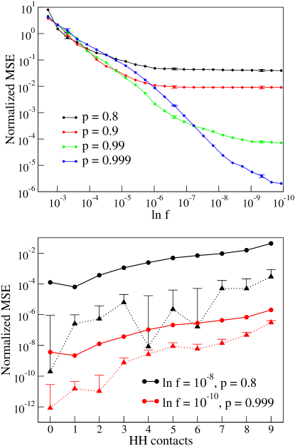
Figure 2: (Color online) Normalized mean square error (NMSE) of DOS estimates for an HP 20mer on the square lattice as a function of modification factor $f$ and flatness criterion $p$. Top: NMSE of $g(E_{\min}=-9)$ vs $\ln f$ for several $p$. Bottom: NMSE over the entire energy range for two pairs of $\ln f_{\text{final}}$ and $p$. The solid lines show the entire NMSE (error bars smaller than symbol size) and the dotted lines (triangles) show the bias terms only.

Fig. 2 shows the normalized mean square error (NMSE) of our estimates of $g(E)$ for the 20mer and the dependence on $f$ and $p$ (results for the 14mer are equivalent). The NMSE is defined as

$$NMSE=\left(\frac{g-\hat{g}}{\hat{g}}\right)^{2}+\frac{1}{N-1}\sum_{i=1}^{N}\left(\frac{g_{i}-g}{g}\right)^{2},$$ (4)

measuring both the systematic (bias term) and statistical (variance term) errors. $\hat{g}$, $g$, and $g_{i}$ stand for the exact, averaged ($N=200$ independent runs have been carried out for statistical reliability) and individual DOS, respectively, at a certain energy $E$.

Both the systematic reduction of the NMSE by decreasing $f$ and increasing $p$ (Fig. 2, top) as well as the very high accuracy achieved over the entire energy range for the most stringent parameter choice ($\ln f_{\text{final}}=10^{-10}$ and $p=0.999$, Fig. 2, bottom) show clear evidence of the correctness of our algorithm and in particular of our “trial-and-error” approach of combined usage of pull, bond-rebridging and pivot Monte Carlo trial moves. Even with $\ln f_{\text{final}}=10^{-8}$ and $p=0.8$, our DOS estimates deviate max. a few percent from the exact values only. (Note that the bias term is generally one to two orders of magnitude smaller than the variance term.)

Reducing $f$ without increasing $p$ leads to a saturation of the NMSE while increasing $p$ without sufficiently decreasing $f$ may result in frozen in systematic errors, see the blue curve in Fig. 2 (top). These findings on short protein sequences suggest that for $p\simeq 0.8$ no further gain in accuracy could be achieved when $\ln f<10^{-6}$, a result in agreement with WL studies of other polymer models.rampf:j_polym_sci_B_polym_phys:06 ; *seaton:phys_rev_E:10 However, for longer sequences we observed that the difficult to access low energy states were often found only during late iterations and large statistical fluctuations in the low energy DOS estimates still remained at $\ln f\approx 10^{-6}$. Only further iterations with reduced $f$ could effectively eliminate such fluctuations. Eventually, the choice $\ln f_{\text{final}}=10^{-8}$ and $p=0.8$ turned out to yield accurate and reliable DOS estimates over the entire energy range at feasible computational costs. This choice of parameters requires three to four orders of magnitude less Monte Carlo trials until convergence of the DOS as compared to the most rigid pair chosen here ($\ln f_{\text{final}}=10^{-10}$ and $p=0.999$).

Final note: The way in which $f$ is decreased affects the accuracy of the final DOS and the time of convergence of the WL procedure. In particular, it has been found that, for constant $p$, decreasing $f$ exponentially (e. g. $\sqrt{f}_{\text{old}}\rightarrow f_{\text{new}}$) eventually leads to saturation in the error of the DOS,belardinelli:phys_rev_E:07 ; zhou:phys_rev_E:08 ; swetnam:j_comput_chem:11 see also Fig. 2 (top). Some promising modifications have been proposed for alleviating this problem, e. g. the $1/t$ algorithmbelardinelli:phys_rev_E:07 or dynamic modification rules for $f$ accounting for the fluctuations in the histogram $H$.zhou:phys_rev_E:08 ; swetnam:j_comput_chem:11 However, no generic ”optimal” rule of reducing $f$ has yet been found without introducing further (unknown) system-type and -size dependent simulation parameters which need to be adjusted in order to make the algorithm effectively converging and outperforming the original approach. For instance, the normalization factor of Monte Carlo time in the $1/t$ algorithm is such a parameter and an improper choice may even lead to non-convergence.swetnam:j_comput_chem:11 The process of finding optimal simulation parameters, however, can become computationally very demanding. On the other hand, our methodological experience for lattice polymers has shown that a good choice of efficient MC trial moves has a much larger impact on the overall performance and efficiency of the WL procedure than such parameter ”tunings”. Therefore, in this study we kept the standard WL rule of reducing $f$ with its proven robustness over a large spectrum of problems.

II.4 Calculation of thermodynamic and structural quantities

Because the energy density of states $g(E)$ does not depend on temperature $T$, an estimate of $g(E)$ allows us to calculate the partition function $Z(T)$ (up to a multiplicative constant), see Eq. (1), and its derived thermodynamic quantities at any temperature. For instance, the internal energy $U(T)$ and specific heat $C(T)$ are obtained as

$$U(T)=\frac{1}{Z(T)}\sum_{E}Eg(E)e^{-E/kT}\equiv\langle E\rangle$$ (5)

and

$$C(T)=\frac{\partial U(T)}{\partial T}=\frac{\langle E^{2}\rangle-\langle E\rangle^{2}}{kT^{2}}.$$ (6)

Besides thermodynamic quantities, structural observables such as the radius of gyration, etc., are equally important to provide insight into the conformational changes taking place with varying temperature. Principally, such structural observables could be sampled simultaneously during the late iterations of the Wang-Landau procedure. Often though, some experimentation is required to find appropriate observables; thus, it may be more convenient to sample them in a second simulation step.

Here, a “Wang-Landau resampling” procedure has been employed, where the final $g(E)$ obtained from WL sampling is further updated (using a small modification factor, $\ln f\leq 10^{-7}$) and the same Monte Carlo acceptance criterion as in Eq. (2) is applied. Alongside the simulation, structural quantities are measured and the sampling stops when all (previously “visited”) bins of the energy histogram $H(E)$ have reached a sufficient number of hits (of the order of $10^{8}$/$10^{9}$). The thermodynamic average of a quantity $Q$ is then obtained from

$$\langle Q\rangle(T)=\frac{1}{Z(T)}\sum_{E}e^{-E/kT}g(E)\overline{Q}(E).$$ (7)

$\overline{Q}(E)$ is the average of $Q$ at energy $E$, i. e.

$$\overline{Q}(E)=\frac{\sum_{Q}QH(E,Q)}{\sum_{Q}H(E,Q)},$$ (8)

where $H(E,Q)$ is the two-dimensional histogram in $E$ and $Q$. Because of its advantageous dynamics, this WL resampling procedure turned out to cover conformational space more uniformly and faster (including conformational regions of low energy) than with standard multicanonical sampling.landau:09 ; *newman:99 However, an accurate estimate of $g(E)$ is essential for this procedure to yield reliable results.

III Results and Discussion

III.1 Ground state search

Various benchmark HP sequences have been designed, either as simplified counterparts to real proteins (e. g. a 103mer for Cytochrome C),lattman:biochemistry:94 or just for the purpose of algorithm testing.unger:5th_procs:93 ; yue:pnas:95b The longest sequence explored systematically so far, contains 136 residues.lattman:biochemistry:94

First, we applied our method to a series of ten 48mers (3D),yue:pnas:95b which has been used extensively for testing of algorithmic efficiency, see Table 1. For each HP sequence we measured the lowest energy found ($E_{\min}$), the time between independent hits of a ground state ($t_{\text{hit}}$, in this study defined as the time of a “round trip”, where a conformation with zero energy must have been visited at least once between two consecutive hits of a ground state) and the time until convergence of the density of states over the entire energy interval $[E_{\min},0]$ ($t_{\text{DOS}}$). For statistical significance, WLS timings depict the interquartile mean of 20 independent WL runs.

Table 1: Comparison of performance for different methods on a series of ten HP sequences with chain lengths $N=48$ in 3D.yue:pnas:95b $E_{\min}$ denotes the minimum energy reported by all methods. Columns 3-5 give the times (in minutes) between independent hits of $E_{\min}$ ($t_{\text{hit}}$). The last column depicts the WL convergence times of the DOS in the energy interval $[E_{\min},0]$ with $\ln f_{\text{final}}=10^{-8}$ and $p=0.8$. For details of nPERMis and FRESS, see Refs. hsu:j_chem_phys:03, ; *hsu:phys_rev_E:03 and zhang:j_chem_phys:07, , respectively; for nPERMis, we only list the timings for the non-biased version.

Seq.	$E_{\min}$	WLS	nPERMis	FRESS	$t_{\text{DOS}}$(WLS)
1	-32	$0.32$	$0.63$	$0.72$	$23.1$
2	-34	$0.84$	$3.89$	$0.88$	$54.9$
3	-34	$0.68$	$1.99$	$0.77$	$28.3$
4	-33	$0.59$	$13.45$	$0.53$	$25.5$
5	-32	$0.23$	$5.08$	$0.72$	$15.5$
6	-32	$0.39$	$6.60$	$0.68$	$21.3$
7	-32	$1.58$	$5.37$	$1.12$	$49.5$
8	-31	$0.58$	$2.17$	$0.80$	$37.4$
9	-34	$3.10$	$41.41$	$0.73$	$63.2$
10	-33	$0.98$	$0.47$	$0.73$	$34.8$

Our findings were compared with two other methods for which timing data are available: (i) an improved variant of the pruned-enriched Rosenbluth method (nPERMis)hsu:j_chem_phys:03 ; *hsu:phys_rev_E:03 and (ii) fragment regrowth Monte Carlo via energy-guided sequential sampling (FRESS).zhang:j_chem_phys:07 Although it is clear that a comparison of timings is always limited because of the different implementations and CPU speeds, it serves, nonetheless, as a good indicator of performance, in particular, when considered among several HP sequences.

nPERMis is a thoroughly tested, “pure” chain-growth algorithm that has been very successful on many HP sequences. It is a generic Monte Carlo sampling scheme able to generate the correct Boltzmann weights. (Another improved PERM variant, nPERMh,huang:phys_rev_E:05 has been exclusively designed for conformational search and is, therefore, excluded here; for the flat histogram/multicanonical PERM versions,prellberg:phys_rev_lett:04 ; bachmann:phys_rev_lett:03 ; *bachmann:j_chem_phys:04 only sparse data are available and unfortunately no timings have been reported.)

In FRESS, Monte Carlo trial moves consist of cutting out and regrowing pieces of variable length along the protein chain. This update scheme yields a very efficient conformational search strategy and, so far, FRESS has been the only method capable of finding putative minimal energies for all commonly studied benchmark HP sequences. However, although principally usable for Boltzmann sampling, it has achieved these results with methodological tuning (“shortcuts”) only, e. g. usage of simulated annealing, neglect of detailed balance, or adoption of a depth-first-search strategy to regrow chain fragments.

Table 1 shows that for these still relatively short sequences, the three methods perform consistently well. They all find the same putative ground states and the timings between independent hits are comparable (although the timings for nPERMis fluctuate considerably more than for WLS and FRESS).

Another series of ten 64mers (3D)unger:5th_procs:93 showed a similar picture (details not shown here). We found the same putative ground state energies as nPERMgrassberger:arxiv:04 and FRESS. Our timings ranged from a few seconds up to around one hour, those for nPERM from a few seconds up to 8 hours (on a 2GHz PC); no timings have been reported for FRESS.

Table 2: Comparison of performance for different methods on benchmark HP sequences with $N>50$ on square (2D) and simple cubic (3D) lattices. For each sequence, the original reference is cited. Columns 3-5 give the times (in hours, except otherwise stated) between independent hits of the respective energy minima $E_{\min}$ ($t_{\text{hit}}$). The last column gives the WL convergence times of the DOS in the energy interval $[E_{\min},0]$ with $\ln f_{\text{final}}=10^{-8}$ and $p=0.8$. For details of nPERMis and FRESS, see Refs. hsu:j_chem_phys:03, ; *hsu:phys_rev_E:03 and zhang:j_chem_phys:07, , respectively. NA means no data available.

Sequence	$E_{\min}$	WLS	nPERMis	FRESS	$t_{\text{DOS}}$(WLS)
2D64 unger:j_mol_biol:93	-42	$<10$s	$30$	$<0.33$	$0.28$
2D85 konig:biosystems:99	-53	$0.03$	$0.17$	$<0.33$	$1.06$
2D100a ramakrishnan:j_chem_phys:97	-48	$0.07$	$0.04$	$<0.33$	$1.51$
2D100b ramakrishnan:j_chem_phys:97	-50	$0.17$	$5.8$	$<0.33$	$2.49$
3D58 dill:pnas:93	-44	$0.12$	$0.19$	$0.09$	$2.23$
3D64 yue:pnas:95a	-56	$0.09$	$0.45$	$0.53$	$2.61$
3D67 yue:pnas:95a	-56	$0.99$	$1.12$	$1.41$	$13.80$
3D88 beutler:protein_sci:96	-69	$0.45$	NA		$8.30$
	-72	$8.92$		$5.03$	$122.86$
3D103 lattman:biochemistry:94	-54	$0.01$	$3.12$		$0.65$
	-57	$0.93$		$4.47$	$9.79$
	-58	NA			NA
3D124 lattman:biochemistry:94	-71	$0.06$	$12.3$		$2.28$
	-75	$\approx 104$		$<14$d	$\geq 10$d
3D136 lattman:biochemistry:94	-80	$2.98$	$110$		$34.17$
	-82	$\approx 89$		$6.42$	$\geq 10$d
	-83	$\geq 10$d		$<14$d	NA

As a more stringent test we have selected particular benchmark HP sequences with $N>50$ in two and three dimensions (for a listing of these sequences, see e. g. Ref. zhang:j_chem_phys:07, ). Table 2 summarizes the results (WLS timings were obtained as above). Overall, the performance of an algorithm is now more sequence dependent but two tendencies are most striking: In 2D, nPERMis shows large timing differences dependent on the HP sequence whereas WLS and FRESS perform much more homogeneously. For longer sequences in 3D ($N\geq 88$), nPERMis performs considerably worse than the other two methods, both in terms of energy minima found as well as in corresponding timings. Difficulties in finding the ground state can sometimes be traced back to certain characteristics of the native structure, e. g. the formation of a very distinct hydrophobic core (3D88) or chain terminals deeply buried in the interior of the structure (2D64);hsu:j_chem_phys:03 ; *hsu:phys_rev_E:03 see the examples of ground state structures for each sequence of Table 2 in Figs. 4, 5 and 6.

Often though, the causes are less apparent and looking at a few single ground state structures is insufficient. Instead, it is necessary to consider the entire ensemble. For instance, the native states for the two 100mers in 2D (2D100a and 2D100b, see Fig. 4), look very similar (as are their minimal energies) and do not feature any peculiarities. Nonetheless, nPERMis shows timing differences of two orders of magnitude between the two sequences whereas WLS and FRESS perform equally well in both cases. In order to better understand this behavior, we have calculated the contact map densities of the ensembles of respective ground states for both sequences, see Fig. 3. The figure illustrates clearly that native structures in case of sequence 2D100a are rather homogeneously distributed in conformational space whereas for sequence 2D100b they are concentrated in fewer but denser locations manifesting a lower degeneracy. As the timings in Table 2 indicate, this difference does not seem to impact the sampling abilities of FRESS and WLS. Owing to their efficient Monte Carlo update schemes, both algorithms can easily traverse between distant regions of conformational space.

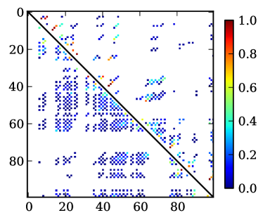
Figure 3: (Color online) Contact map density of ground states for the sequence 2D100a (lower triangle, $E_{\min}=-48$) and 2D100b (upper triangle $E_{\min}=-50$), respectively. For each sequence, densities have been calculated from a sample of more than 10,000 contact maps of ground states contributed from 20 independent WL production runs. Only non-vanishing HH contact densities are shown.

In contrast, nPERMis needs much more time to explore different portions of conformational space, once growth proceeds far in one direction (despite sophisticated pruning/enrichment mechanisms). This problem becomes more severe for longer sequences and denser sampled conformational spaces. Therefore, we conjecture that this is also the main cause of troubles for the longer sequences in 3D. Even though stronger heuristicsbeutler:protein_sci:96 ; hsu:j_chem_phys:03 ; *hsu:phys_rev_E:03; huang:phys_rev_E:05 or flat-histogram/multicanonical approachesprellberg:phys_rev_lett:04 ; bachmann:phys_rev_lett:03 ; *bachmann:j_chem_phys:04 may partially alleviate these difficulties, the problem remains inherent in any static chain-growth algorithm (i. e. one that always grows from the same starting point) when sampling the generally dense conformational spaces at low temperature. The apparent tendencies exposed by this comparison of methods in Table 2 clearly contradict the statements in Ref. bachmann:phys_rev_lett:03, ; *bachmann:j_chem_phys:04 where it has been argued that chain-growth algorithms perform better than Monte Carlo algorithms employing trial moves in simulating lattice proteins at low temperatures. This contradiction stems from the fact that the latter methods, such as Wang-Landau sampling, strongly depend on the chosen trial move set; a point likely not given enough attention in Ref. bachmann:phys_rev_lett:03, ; *bachmann:j_chem_phys:04.

With our strategy, we were able to find all currently known putative ground state energies for these benchmark HP sequences, inclusive a conformation with energy $-58$ for the sequence 3D103. This result has also been obtained by constrained-based protein structure prediction (CPSP).backofen:constraints:06 However, CPSP is not a “blind” search algorithm but rather based on the threading of a sequence through a set of pre-calculated compact hydrophobic cores. Thus, it can also not yield thermodynamic properties and is not applicable to two-dimensional systems where native structures do not necessarily form compact H-cores. To our knowledge, our procedure is the only generic and fully blind Monte Carlo sampling scheme achieving these results so far.

Sequence 3D103 demonstrates particularly well the algorithmic improvements (not just increase of CPU speed) that have been achieved in the course of time. In 1994, Lattman et al.lattman:biochemistry:94 proposed a first ground state energy $E=-44$ by means of hydrophobic zipper. The sequence then served as a testing ground for various methods, ranging from contact interactionstoma:protein_sci:96 ($E=-49$), PERM variantshsu:j_chem_phys:03 ; *hsu:phys_rev_E:03; bachmann:phys_rev_lett:03 ($E=-54,-55,-56$), FRESSzhang:j_chem_phys:07 ($E=-57$) to WLSwuest:phys_rev_lett:09 ($E=-58$). Due to insufficient sampling of the ground state we could not obtain an estimate of the relative DOS between the ground and first excited states, but we certainly now know that the probability of finding a conformation with energy $E=-58$ is definitely more than 20 orders of magnitude smaller than for a conformation with $E=-44$.

III.2 Thermodynamic properties

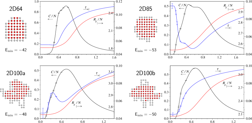
Figure 4: (Color online) Specific heat, $C/N$ (black curves, left ordinates), and canonical ensemble averages of the root mean squared radius of gyration, $R_{g}/N$ (red curves, outer right ordinates), and tortuosity, $\tau$ (blue curves, inner right ordinates), as a function of temperature (abscissas: $kT/\epsilon$) for several benchmark HP sequences on the square lattice (2D). For each sequence, $C$ has been obtained from the average DOS of 20 independent WL simulations in the corresponding energy interval $[E_{\min},0]$, and $R_{g}$, $\tau$ from 20 independent WL resampling production runs. Errors have been estimated by means of a bootstrap analysislandau:09 ; *newman:99 with 200 resamples and are shown where visible only. For each sequence, a typical ground state conformation is shown on the left with red and light-gray beads indicating hydrophobic (H) and polar (P) residues, respectively. For further explanations, see text.

With regard to conformational search, the robustness ($E_{\min}$’s found) and performance (timings) of FRESS and our approach are very much alike with some sequence-dependent differences. The main advantage of our approach over FRESS, however, lies in the usage of a simpler, but equally efficient, Monte Carlo trial move set which can be readily combined with Wang-Landau sampling. This strategy allowed us not only to find putative ground states but, at the same time, to obtain estimates of the DOS with very high accuracy ($\ln f_{\text{final}}=10^{-8}$ and $p=0.8$). The DOS gives access to thermodynamic quantities over the whole temperature range and, in particular, enables us to better explore the intricate folding behavior of these model proteins at low temperatures.

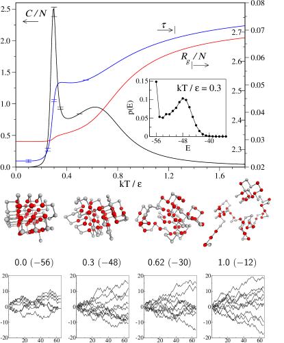
Figure 5: (Color online) Main figure: Same as Fig. 4 for an HP 67mer on the simple cubic lattice (3D).yue:pnas:95a The inset figure shows the canonical energy distribution, $p(E)$, at the temperature where $C$ takes its maximum in the sharp peak. Below, typical structures are shown at indicated temperatures and energies ($kT/\epsilon$, $E$). The native state of this sequence ($E_{\min}=-56$) resembles an $\alpha$/$\beta$-barrel in real proteins. The ground state and the structure with $E=-48$ correspond to the two maxima of the bimodal distribution of $p(E)$ in the inset figure illustrating the significant conformational rearrangements taking place at the folding transition. Each of the small figures at the bottom shows the “winding walks” [$s_{i}$ vs $i$, see Eq. (10)] of 10 structures at corresponding energies. For further explanations, see text.

Figs. 4, 5 and 6 show the specific heats, $C$ (see Eq. 6), as a function of temperature ($T$) for the HP sequences of Table 2. In free space (as studied here), the $C$ curves of most sequences exhibit two major transitions:

(i) At high $T$, a wide peak in $C$ indicates the collapse of the protein from a swollen coil to a compact globular (pseudo-) phase; see also the snapshots of structures at $kT/\epsilon=1.0$ and $kT/\epsilon=0.62$ in Fig. 5. (Note that the term “phase” is actually not strictly defined as we are considering systems of finite size only.) Since the structures in both phases are still of a random nature, the location of this transition ($T_{c}$ of specific heat maximum) shows little sequence dependency (at least for these still relative short protein-like sequences, see also Sec. III.3). It depends, however, on the fraction of H monomers in the sequence. This explains, for instance, the very similar transition temperatures of sequences 2D100a ($T_{c}\approx 0.49$, 55% H) and 2D100b ($T_{c}\approx 0.48$, 56% H) and the higher one for sequence 2D85 ($T_{c}\approx 0.65$, 69.4% H). A higher fraction of H residues raises the collapse transition temperature because of the generally larger number of HH contacts which need to be broken upon going from a globular to a coil structure; see also the discussion in Ref. kou:j_chem_phys:06, .

(ii) At low $T$, the specific heat signals another transition which manifests the folding of the protein from a random globule to its native state(s). Shape, magnitude and location of this transition are all very sequence dependent; the curves of $C$ range from a barely visible shoulder (2D100a, Fig. 4) to a very sharp peak with a clear first-order-like bimodal energy distribution (3D67, see also the inset figure and the typical structures at the lower two temperatures in Fig. 5). Low ground state degeneracy or energy gaps may give some indication about the nature of this transition. But ultimately, it is only the entire low energy range of the DOS which determines the exact character of this transition. Therefore, accurate sampling of the low energy range is compulsory to gain a conclusive picture of the low temperature folding behavior. Otherwise, important features of some sequences do not show up at all (e. g. the sharp peak in the specific heat of sequence 3D88 in Fig. 6, indicating a pronounced folding transition which leaves the coil-globule transition as only a flat shoulder remnant).

None of the HP sequences studied here has an energy gap between ground and excited states; such a gap has been considered a prerequisite of a good folder (i. e. having a pronounced global energy minimum).sali:nature:94 However, the longest two sequences show very sharp drops (several orders of magnitude) in the DOS between first excited and ground state (3D124) or between the lowest excited states (3D136). These “kinks” in the DOS cause the sharp, low $T$ specific heat peaks. For sequence 3D124, this is the only signal in the low temperature regime (no folding transition). The folding transition of sequence 3D136 is located near $kT/\epsilon\approx 0.35$; below this $T$, two excitation transitions occur (a weak and a very sharp near $T\rightarrow 0$). Clearly, the locations and amplitudes of these very low $T$ peaks in $C$ are somewhat uncertain.

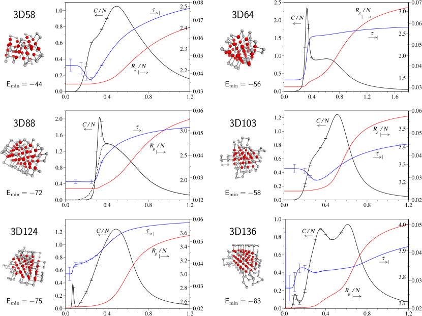
Figure 6: (Color online) Same as Fig. 4 for several benchmark HP sequences on the simple cubic lattice (3D). For sequence 3D88, the dashed line shows the specific heat ($C/N$) calculated from the DOS with energy range $[-69,0]$ only. For sequences 3D103 and 3D136, the DOS/observables have been only obtained for the energy ranges $[-57,0]$ and $[-82,0]$, respectively, because of the difficulty to sample the respective ground states. Since $\tau$ is very sensitive at low $T$, for sequences with $N>100$, structural observables have been averaged from 50 independent WL production runs.

Beside the specific heat, structural quantities have been calculated to get further insight into the folding process. For instance, the root mean squared radius of gyration, $R_{g}$,

$$R_{g}=\left(\frac{1}{N}\sum_{i}^{N}(\bm{r}_{i}-\bm{r}_{cm})^{2}\right)^{1/2},$$ (9)

($\bm{r}_{i}$ is the position vector of the $i^{\text{th}}$ monomer and $\bm{r}_{cm}$ is the center of mass), is known to be a well suited observable to signal the collapse of homo- and heteropolymers.bachmann:j_chem_phys:04 ; rampf:j_polym_sci_B_polym_phys:06 ; *seaton:phys_rev_E:10 Our figures (red curves in Figs. 4, 5 and 6) confirm this observation and show a clear coincidence between the upper maximum in $C$ and the strong decay of $R_{g}$. Due to finite size effects,sharma:j_chem_phys:08 the steepest slope of $R_{g}$ is slightly shifted towards higher $T$ as compared to the specific heat maximum ($T_{c}$). On the other hand, $R_{g}$ shows little or no signal in the low temperature regime. The polymer end-to-end distance, $R_{e}$ (not shown here), has very similar properties as $R_{g}$ and shows the same S-shaped curve indicating the collapse. At low $T$, $R_{e}$ may have a minimum and rise again as $T\rightarrow 0$. This effect is more pronounced for HP sequences with P terminals signaling the tendency to push P monomers towards the surface in order to maximize the formation of a compact hydrophobic core.bachmann:j_chem_phys:04 However, measuring the spatial extent of a polymer only, $R_{g}$, $R_{e}$, or similar properties like e. g. box size or surface P number,kou:j_chem_phys:06 are insensitive to the sequence specific internal conformational (and topological) changes taking place upon folding from the globular denatured states to the ground state.

Measures of conformational “distance” to the native state, based on an adjacency matrixchan:j_chem_phys:94 or the number of native contacts (e. g. the Jaccard index),jaccard:01 ; wuest:phys_rev_lett:09 may better serve as a reaction coordinate. However, for sufficiently long chains, calculations of such measures can become computationally intractable and they may also bear some ambiguity (e. g. dependence on the choice of move set or large degeneracy of the native state). Moreover, a requirement of these observables is that the native state(s) being effectively known to give meaningful results. Thus, it still remains a challenge to “design” a (computationally affordable) structural observable which reflects the cooperative rearrangements and activity indicated by the peaks or shoulders in the specific heats at low $T$.

Based on the ideas of the “DNA walk”,buldyrev:dna_walk:94 we propose here a scalar structural observable which might provide better insight into the internal topological changes taking place upon folding. We define the tortuosity (or writhing/winding measure) of the protein as

$$\tau=\left(\frac{1}{N-2}\sum_{i=1}^{N-2}(s_{i}-\bar{s})^{2}\right)^{1/2},$$ (10)

where

$$s_{i}=\sum_{j=1}^{i}\bm{r}_{j,j+1}\times\bm{r}_{j,j+2},\quad 1\leq i\leq N-2.$$ (11)

$\bm{r}_{j,j+1}$ and $\bm{r}_{j,j+2}$ denote the two-dimensional vectors between monomers $(j,j+1)$ and $(j,j+2)$, respectively (in the plane spanned by these three monomers). Their cross product determines whether two consecutive bonds define a left ($-1$) or right ($+1$) turn or are collinear ($0$).cormen:09 $s_{i}$ is the running sum of bond turns along the polymer chain (“winding walk”); examples of $s_{i}$ for some conformations at different energies are shown at the bottom of Fig. 5. The standard deviation of $s_{i}$, here denoted as $\tau$, is thus a measure of polymer tortuosity. (Note that $\tau$ is invariant to the direction of the running sum $s_{i}$ along the chain.)

The blue curves in Figs. 4, 5 and 6 display $\tau$ as a function of $T$. Overall, they reveal the following picture: By lowering $T$, the associated contraction of the protein results in a reduction of conformational degrees of freedom and, thus, in a decrease of “winding freedom” as well. At a certain point in the low temperature regime, $\tau$ undergoes a significant change, showing a sharp drop-off (increase) or passing over a rounded peak (through). The diversity of signals is a consequence of the different sequences of H and P residues as well as the different chain lengths. But the important observation is that the temperature region of this change clearly does not coincide with the collapse transition (where the protein’s shape is still random) but with the low temperature signal in the specific heat (i. e. the folding transition). At this temperature, internal structural rearrangements take place (e. g. breaking of HH contacts of compact denatured states) which eventually allow the protein to assume its native state. Being sensitive to exactly such topological transformations, $\tau$ reflects this folding behavior. It serves, thus, as a complementary structural quantity to better interpret the thermodynamic activity observed in the specific heats. It might be conjectured that the shape of $\tau$ could even give some deeper insight into the folding characteristics, such as a sharp drop of $\tau$ indicating a folding funnel or a peak signaling a folding barrier. Furthermore, the standard deviation is just one (simple) means of analyzing the “winding walks” $s_{i}$ and other, more appropriate, measures could be conceived. These questions are left for further research.

III.3 Random vs protein-like HP heteropolymers

Many of the above HP sequences (Figs. 4, 5 and 6) have been derived from real proteins and mimic protein-like behavior exhibiting some kind of collapse and folding transitions. However, for these relatively short chains ($N\leq 100$), the characteristics and strengths of the two transitions are highly sequence dependent and subject to strong surface effects in the folded state (for a perfect cube of $N=125$, only about 20% of the monomers are in the bulk). Although there is no thermodynamic limit in the exact statistical sense for any single heteropolymer, here we are interested in identifying the generic differences between random and protein-like HP sequences in the long-chain limit.

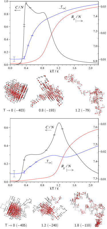
Figure 7: (Color online) Comparison of thermodynamic ($C$) and structural ($R_{g},\tau$) properties between a random (top) and protein-like (bottom) HP heteropolymer. Both sequences constitute 500 monomers with a 50% : 50% ratio among H and P. For both sequences, typical structures are shown at indicated temperatures and energies ($kT/\epsilon$, $E$).

To address this question, we have studied several long ($N=500$) HP chains, each with 50% H and 50% P monomers in either random or protein-like sequence. The latter have been constructed as follows:boelinger:08 Starting from a compact, globular homopolymer conformation (i. e. only H), the 50% of monomers which are farthest from the center of mass are marked as P (polar). Repeating this process for different homopolymer conformations yields protein-like HP sequences with distinct hydrophobic cores. Longer HP polymers allowed us also to further test the efficiency of our procedure. By splitting up the calculation of the DOS into two unequal energy windows (the lower one covering only 10-15% of the entire energy interval with sufficient overlap to the larger window by e. g. 25 energy levels), we could accurately estimate the DOS over more than 95% of the entire energy range of these sequences within a couple of CPU days. Note that for these chain lengths, finding the ground state is currently still out of reach for any method due to the exponentially increasing computational complexity; but this is not a requirement here.

An important dissimilarity between random and protein-like sequences becomes already visible in the DOS: For given ratios of H and P monomers, both types of sequences span roughly the same energy range (here $E_{\min}\approx-400$) but the DOS is steeper at low energies for protein-like sequences. This behavior is in agreement with the notion of folding funneldill:protein_sci:99 where the occupied conformational space of a protein abruptly reduces when approaching the native state.

Another difference arises in their thermodynamic and structural behaviors. As shown in Fig. 7 the collapse transition for the protein-like heteropolymer is significantly shifted towards higher $T$ as compared to the random sequence ($T_{c}\approx 1.2$ and $T_{c}\approx 0.9$, respectively). This can be rationalized by the “design” of the protein-like sequences favoring the formation of hydrophobic cores already at $T_{c}$, with a significantly lower energy compared to the random case (see the corresponding structures with energies $-240$ and $-193$, respectively). Interestingly, however, among sequences of the same type (i. e. either random or protein-like), $T_{c}$ shows only little variation. For both sequences, the drop-off of $R_{g}$ coincides generally better with the upper specific heat peak (collapse transition) as compared to the shorter HP sequences studied above.

The specific heat of the protein-like sequence shows a clear separation between collapse and folding transition (although the latter is often manifested by a shoulder only) exemplifying a rough but structured energy landscape. The course of the winding measure ($\tau$) corroborates this observation signaling a division between collapse and folding phase. In contrast, for the random heteropolymer, the two transitions are more interleaved, and the collapse transition is largely suppressed by the generally stronger transition to the ground state. This is a consequence of the inability to form a hydrophobic core and the absence of conformational “guidance” (folding path) towards the ground state. Although $\tau$ features also a more or less pronounced drop-off, its occurrence does not coincide with the low $T$ peak in the specific heat anymore (as observed for some of the shorter protein-like HP sequences above).

A systematic analysis of these observations, by considering a large ensemble of HP sequences, would be both a computational challenge and an interesting topic to better understand the generic behavior of these model proteins.

IV Conclusion

We have presented a generic Monte Carlo scheme based on Wang-Landau sampling with suitable trial moves (combination of pull, bond-rebridging and pivot moves) which is very efficient for the simulation of HP lattice proteins and the analysis of their thermodynamic properties over the entire temperature range. Because of its intrinsic simplicity and flexibility, our method is ideally suited for the many variations of this common protein model, e. g. protein adsorption,li:comput_phys_commun:11 ; li:12 protein aggregation and the like. For instance, with our present, optimized, algorithm, it takes only about 5.5 hours ($t_{\text{DOS}}$) to obtain the entire DOS of an HP 36mer adsorbing on a weakly attracting surface (i. e. between one to two orders of magnitude faster than in Ref. li:comput_phys_commun:11, ). This system has been used as a benchmark to demonstrate the efficiency of a recently proposed Wang-Landau scheme coupled with configurational bias Monte Carlo which achieved $t_{\text{DOS}}\approx 28$h under the same conditions.radhakrishna:j_chem_phys:12 Besides considerable higher performance, the main advantage of our approach is that its efficiency does not depend on the tuning of external simulation parameters (e. g. an unphysical temperature as in Ref. radhakrishna:j_chem_phys:12, ). Our approach has also proven powerful for exploring the low-temperature thermodynamics of interacting self-avoiding walks, even for chain lengths $N\gg 1000$.wuest:phys_rev_lett:09 ; wuest:isaw

Among the various ingredients used to tackle simulations of lattice proteins or polymers at low temperatures and high densities, ranging from the Monte Carlo driver to various tuning schemes, it turned out that the use of appropriate Monte Carlo trial moves has the greatest impact on the overall performance and accuracy of the algorithm. However, we stress that it is the interplay between Wang-Landau sampling, trial move set and efficient implementation which ultimately resulted in the overall robustness and performance of our approach.

Substantial further efficiency improvements would likely be gained with suitable parallelization techniques. Subdivision of the sampling of the DOS into smaller energy windows or the use of multiple random walkers which simultaneously update a single DOS are two already well studied approaches in this direction.zhan:comput_phys_commun:08 A more advanced and interesting parallelization scheme would allow exchange of conformations among several independently running Wang-Landau samplers, similar to the ideas employed in parallel tempering.landau:09 ; *newman:99 Such “conformational mixing” could considerably reduce the tunneling time of a random walk between the energy boundaries and thus speed up the overall convergence of the simulation.

- (1) K. A. Dill, Protein Sci. 8, 1166 (1999)
- (2) A. Kolinski and J. Skolnick, Polymer 45, 511 (2004)
- (3) K. A. Dill, Biochemistry 24, 1501 (1985)
- (4) K. F. Lau and K. A. Dill, Macromolecules 22, 3986 (1989)
- (5) A. Sali, E. I. Shakhnovich, and M. Karplus, Nature 369, 248 (1994)
- (6) E. I. Shakhnovich, Curr. Opin. Struct. Biol. 7, 29 (1997)
- (7) T. Cellmer, D. Bratko, J. M. Prausnitz, and H. Blanch, Proc. Natl. Acad. Sci. USA 102, 11692 (2005)
- (8) L. Zhang, D. Lu, and Z. Liu, Biophys. Chem. 133, 71 (2008)
- (9) V. Castells, S. Yang, and P. R. V. Tassel, Phys. Rev. E 65, 031912 (2002)
- (10) M. Bachmann and W. Janke, Phys. Rev. E 73, 020901(R) (2006)
- (11) M. Radhakrishna, S. Sharma, and S. K. Kumar, J. Chem. Phys. 136, 114114 (2012)
- (12) D. Gersappe, W. Li, and A. C. Balazs, J. Chem. Phys. 99, 7209 (1993)
- (13) R. Bonaccini and F. Seno, Phys. Rev. E 60, 7290 (1999)
- (14) V. P. Zhdanov and B. Kasemo, Proteins 42, 481 (2001)
- (15) G. Ping, J. M. Yuan, M. Vallieres, H. Dong, Z. Sun, Y. Wei, F. Y. Li, and S. H. Lin, J. Chem. Phys. 118, 8042 (2003)
- (16) P. F. N. Faísca, R. D. M. Travasso, T. Charters, A. Nunes, and M. Cieplak, Phys. Biol. 7, 016009 (2010)
- (17) F. Rampf, K. Binder, and W. Paul, J. Polym. Sci. B Polym. Phys. 44, 2542 (2006)
- (18) D. T. Seaton, T. Wüst, and D. P. Landau, Phys. Rev. E 81, 011802 (2010)
- (19) J. L. Zhang and J. S. Liu, J. Chem. Phys. 117, 3492 (2002)
- (20) E. M. O’Toole and A. Z. Panagiotopoulos, J. Chem. Phys. 97, 8644 (1992)
- (21) T. C. Beutler and K. A. Dill, Protein Sci. 5, 2037 (1996)
- (22) P. Grassberger, Phys. Rev. E 56, 3682 (1997)
- (23) H. Frauenkron, U. Bastolla, E. Gerstner, P. Grassberger, and W. Nadler, Phys. Rev. Lett. 80, 3149 (1998)
- (24) U. Bastolla, H. Frauenkron, E. Gerstner, P. Grassberger, and W. Nadler, Proteins 32, 52 (1998)
- (25) H.-P. Hsu, V. Mehra, W. Nadler, and P. Grassberger, J. Chem. Phys. 118, 444 (2003)
- (26) H.-P. Hsu, V. Mehra, W. Nadler, and P. Grassberger, Phys. Rev. E 68, 021113 (2003)
- (27) T. Prellberg and J. Krawczyk, Phys. Rev. Lett. 92, 120602 (2004)
- (28) M. Bachmann and W. Janke, Phys. Rev. Lett. 91, 208105 (2003)
- (29) M. Bachmann and W. Janke, J. Chem. Phys. 120, 6779 (2004)
- (30) S. C. Kou, J. Oh, and W. H. Wong, J. Chem. Phys. 124, 244903 (2006)
- (31) Y. Iba, G. Chikenji, and M. Kikuchi, J. Phys. Soc. Jpn. 67, 3327 (1998)
- (32) G. Chikenji, M. Kikuchi, and Y. Iba, Phys. Rev. Lett. 83, 1886 (1999)
- (33) J. Zhang, S. C. Kou, and J. S. Liu, J. Chem. Phys. 126, 225101 (2007)
- (34) B. Berger and T. Leighton, J. Comput. Biol. 5, 27 (1998)
- (35) P. Crescenzi, D. Goldman, C. Papadimitriou, A. Piccolboni, and M. Yannakakis, J. Comput. Biol. 5, 423 (1998)
- (36) R. Unger and J. Moult, J. Mol. Biol. 231, 75 (1993)
- (37) R. König and T. Dandekar, Biosystems 50, 17 (1999)
- (38) F. Liang and W. H. Wong, J. Chem. Phys. 115, 3374 (2001)
- (39) A. Shmygelska and H. H. Hoos, BMC Bioinformatics 6, 30 (2005)
- (40) R. Backofen and S. Will, Constraints 11, 5 (2006)
- (41) T. Wüst and D. P. Landau, Comput. Phys. Commun. 179, 124 (2008)
- (42) T. Wüst and D. P. Landau, Phys. Rev. Lett. 102, 178101 (2009)
- (43) F. Wang and D. P. Landau, Phys. Rev. Lett. 86, 2050 (2001)
- (44) F. Wang and D. P. Landau, Phys. Rev. E 64, 056101 (2001)
- (45) C. Zhou, T. C. Schulthess, S. Torbrügge, and D. P. Landau, Phys. Rev. Lett. 96, 120201 (2006)
- (46) S. Torbrügge and J. Schnack, Phys. Rev. B 75, 054403 (2007)
- (47) C. Gervais, T. Wüst, D. P. Landau, and Y. Xu, J. Chem. Phys. 130, 215106 (2009)
- (48) A. Tröster and C. Dellago, Phys. Rev. E 71, 066705 (2005)
- (49) Y. W. Li, T. Wüst, D. P. Landau, and H. Q. Lin, Comput. Phys. Commun. 177, 524 (2007)
- (50) A. D. Sokal, in Monte Carlo and Molecular Dynamics Simulations in Polymer Science, edited by K. Binder (Oxford University Press, New York, Oxford, 1995) Chap. 2, p. 47
- (51) N. Madras and A. D. Sokal, J. Stat. Phys. 47, 573 (1987)
- (52) N. Madras and A. D. Sokal, J. Stat. Phys. 50, 109 (1988)
- (53) N. Lesh, M. Mitzenmacher, and S. Whitesides, in Proceedings of the 7th Annual International Conference on Research in Computational Molecular Biology (2003) p. 188
- (54) J. M. Deutsch, J. Chem. Phys. 106, 8849 (1997)
- (55) P. V. K. Pant and D. N. Theodorou, Macromolecules 28, 7224 (1995)
- (56) R. Ramakrishnan, B. Ramachandran, and J. F. Pekny, J. Chem. Phys. 106, 2418 (1997)
- (57) C. Zhou and R. N. Bhatt, Phys. Rev. E 72, 025701(R) (2005)
- (58) C. Zhou and J. Su, Phys. Rev. E 78, 046705 (2008)
- (59) A. D. Swetnam and M. P. Allen, Phys. Chem. Chem. Phys. 11, 2046 (2009)
- (60) M. Matsumoto and T. Nishimura, ACM T. Model. Comput. S. 8, 3 (1998)
- (61) M. Lüscher, Comput. Phys. Commun. 79, 100 (1994)
- (62) See http://www.gnu.org/software/gsl/
- (63) M. Bachmann and W. Janke, Acta Phys. Pol. B 34, 4689 (2003)
- (64) R. E. Belardinelli and V. D. Pereyra, Phys. Rev. E 75, 046701 (2007)
- (65) A. D. Swetnam and M. P. Allen, J. Comput. Chem. 32, 816 (2011)
- (66) D. P. Landau and K. Binder, A Guide to Monte Carlo Simulations in Statistical Physics, 3rd ed. (Cambridge University Press, Cambridge, UK, 2009)
- (67) M. E. J. Newman and G. T. Barkema, Monte Carlo Methods in Statistical Physics (Clarendon Press, Oxford, 1999)
- (68) E. E. Lattman, K. M. Fiebig, and K. A. Dill, Biochemistry 33, 6158 (1994)
- (69) R. Unger and J. Moult, in Procs. 5th Int’l. Conf. on Genetic Algorithms (1993) p. 581
- (70) K. Yue, K. M. Fiebig, P. D. Thomas, H. S. Chan, E. I. Shakhnovich, and K. A. Dill, Proc. Natl. Acad. Sci. USA 92, 325 (1995)
- (71) W. Huang, Z. Lü, and H. Shi, Phys. Rev. E 72, 016704 (2005)
- (72) P. Grassberger, arXiv:cond-mat/0408571
- (73) K. A. Dill, K. M. Fiebig, and H. S. Chan, Proc. Natl. Acad. Sci. USA 90, 1942 (1993)
- (74) K. Yue and K. A. Dill, Proc. Natl. Acad. Sci. USA 92, 146 (1995)
- (75) WSL timings for the energies -75 (3D124) and -82, -83 (3D136) have been obtained from WL simulations using already initial DOS estimates from preceding runs which effectively found these energies.
- (76) L. Toma and S. Toma, Protein Sci. 5, 147 (1996)
- (77) S. Sharma and S. K. Kumar, J. Chem. Phys. 129, 134901 (2008)
- (78) H. S. Chan and K. A. Dill, J. Chem. Phys. 100, 9238 (1994)
- (79) P. Jaccard, Bull. Soc. Vaud. Sci. Nat. 37, 547 (1901)
- (80) S. V. Buldyrev, A. L. Goldberger, S. Havlin, C.-K. Peng, and H. E. Stanley, in Fractals in Science, edited by A. Bunde and S. Havlin (Springer, Berlin, 1994) p. 49
- (81) T. H. Cormen, C. E. Leiserson, R. L. Rivest, and C. Stein, Introduction to Algorithms, 3rd ed. (The MIT Press, Cambridge, MA, 2009)
- (82) D. Bölinger, Topologische Untersuchungen von Proteinen, Homo- und Heteropolymeren, Master’s thesis, Johannes Gutenberg University, Mainz, Germany (2008)
- (83) Y. W. Li, T. Wüst, and D. P. Landau, Comput. Phys. Commun. 182, 1896 (2011)
- (84) Y. W. Li, T. Wüst, and D. P. Landau, submitted to Phys. Rev. E
- (85) T. Wüst and D. P. Landau, to be published
- (86) L. Zhan, Comput. Phys. Commun. 179, 339 (2008)