Sheared Ising models in three dimensions

Abstract

The nonequilibrium phase transition in sheared three-dimensional Ising models is investigated using Monte Carlo simulations in two different geometries corresponding to different shear normals. We demonstrate that in the high shear limit both systems undergo a strongly anisotropic phase transition at exactly known critical temperatures $T_{\mathrm{c}}$ which depend on the direction of the shear normal. Using dimensional analysis, we determine the anisotropy exponent $\theta=2$ as well as the correlation length exponents $\nu_{\parallel}=1$ and $\nu_{\perp}=1/2$. These results are verified by simulations, though considerable corrections to scaling are found. The correlation functions perpendicular to the shear direction can be calculated exactly and show Ornstein-Zernike behavior.

1 Introduction

While the occurrence of nonequilibrium phase transitions is ubiquitous in nature, its investigation in the framework of nonequilibrium statistical mechanics is intricate and restricted to a few simple models, like the driven lattice gas (DLG) [1, 2, 3] or, recently, to the driven two-dimensional Ising model [4]. In this model the system is cut into two halves parallel to one axis and moved along this cut with the velocity $v$. The model exhibits energy dissipation and subsequently friction due to spin correlations, which also occurs in a suitable Heisenberg model [5, 6, 7, 8] and, of interest for the current context, undergoes a nonequilibrium (surface) phase transition. The latter has been investigated analytically and with Monte Carlo (MC) simulations for various geometries [9]. Since then, this model has been generalized to the driven Potts models [10], and finite-size effects were calculated analytically in the driven Ising chain [11].

A lot of similarities and comparable critical behavior between the Ising model with friction and the very famous and well investigated DLG have been found [12]. Both models are characterized by a critical temperature $T_{\mathrm{c}}$, which increases with the driving strength, the field and the shift or shear velocity $v$, respectively, and saturates in the high driving limit. For diverse geometries of the Ising model with friction, the critical temperature has been calculated analytically for $v\rightarrow\infty$ [9].

Moreover it was discovered that the DLG and two-dimensional sheared Ising systems with non-conserved order parameter [13, 14, 12] show strongly anisotropic critical behavior, with direction dependent correlation length exponents $\nu_{\parallel}$ and $\nu_{\perp}$. For the $2\mathrm{d}$ and $1{+}1\mathrm{d}$ geometry of the Ising model with shear the same exponents $\nu_{\parallel}=3/2$ and $\nu_{\perp}=1/2$ [12] as in the two-dimensional DLG have been determined. Additionally finite velocities $v$ have been studied and it was found that for all finite $v$ the $2\mathrm{d}$ and $1{+}1\mathrm{d}$ model cross-over from isotropic Ising like behavior to strongly anisotropic mean-field behavior in the thermodynamic limit, demonstrating that the external drive is a relevant perturbation.

In the following we extend the investigations to three-dimensional models in two different shear geometries and focus on the high shear velocity limit $v\rightarrow\infty$. Both represent three-dimensional sheared models and they are therefore experimentally accessible in the framework of sheared binary liquids [15, 16, 17, 18], albeit the order parameter is not conserved here. Using dimensional analysis, we predict the correlation length exponents for arbitrary dimension $d$. These predictions are verified by simulations, however we find strong corrections to scaling at small system sizes.

2 Model

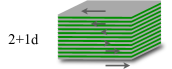
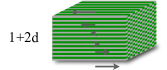
Figure 1: Sketches of the systems considered in this work. On the left hand side the 2+1d system and on the right hand side the 1+2d system is shown. The gray regions represent the magnetic systems and the green (dark) regions are the moving boundaries, while the arrows indicate the motion of the subsystems.

The systems considered in this work are denoted $2{+}1\mathrm{d}$ and $1{+}2\mathrm{d}$ and are shown in Fig. 1, for a classification see Ref. [9]. In the $2{+}1\mathrm{d}$ geometry shear is applied such that two-dimensional Ising models are moved relative to their upper (lower) neighboring layer with velocity $v$ ($-v$) along an axis. In the following we denote the direction parallel to the shear with $\parallel$, the direction perpendicular to the planes with $\perp_{1}$ and the inplane direction perpendicular to the shear direction with $\perp_{2}$. The model contains $L_{\perp_{1}}\times L_{\perp_{2}}\times L_{\parallel}$ spins (lattice sites), where we choose $L_{\perp_{1}}=L_{\perp_{2}}=:L_{\perp}$ throughout this work, and periodic boundary conditions are applied in all directions. The shear velocity $v$ corresponds to a shear rate, which is often denoted as $\dot{\gamma}$ [13, 14]. Using the notation $(\perp_{1}\,\perp_{2}\,\parallel)$ for directions, the shear is in $(001)$-direction and the shear normal is in $(100)$-direction.

A finite shear velocity $v$ is implemented by shifting neighboring layers $v$ times by one lattice constant during one MC step (for details see [4, 9]). A simplification of the implementation is yielded by reordering the couplings between moved layers instead, and by introducing a time-dependent displacement $\Delta(t)=vt$ we get the Hamiltonian

$$\beta\mathcal{H}(t) = -\sum_{k=1}^{L_{\perp_{1}}\vphantom{L_{\parallel}}}\sum_{l=1}^{L_{\perp_{2}}\vphantom{L_{\parallel}}}\sum_{m=1}^{L_{\parallel}}\sigma_{klm}\Big{(}K_{\parallel}\sigma_{k,l,m+1}+$$ (1)

$${}+K_{\perp_{2}}\sigma_{k,l+1,m}+K_{\perp_{1}}\sigma_{k+1,l,m+\Delta(t)}\Big{)},$$

where $K_{\mu}=\beta J_{\mu}$ is the reduced nearest neighbor coupling with $\mu=\{\perp_{1},\perp_{2},\parallel\}$, and $\beta=1/k_{\mathrm{B}}T$. In the following we concentrate on the infinite shear velocity limit $v\to\infty$, which can easily be implemented by choosing $1\leq\Delta(t)\leq L_{\parallel}$ randomly. In this limit an analytical calculation [9] yield the equation

$$\chi_{\mathrm{eq}}^{(0)}(K_{\mathrm{c},\parallel})f\tanh K_{\mathrm{c},\perp}=1$$ (2)

from which we can determine the critical temperature, where $\chi_{\mathrm{eq}}^{(0)}$ is the zero field equilibrium susceptibility of the subsystems moved relative to each other and $f$ the number of fluctuating adjacent fields. Here $\chi_{\mathrm{eq}}^{(0)}$ of the two-dimensional Ising model is required, which has been calculated to higher than $2000^{\mathrm{{th}}}$ order by an polynomial algorithm [19]. Using $f=2$ and $J_{\parallel}=J_{\perp_{1}}=J_{\perp_{2}}=1$ we get

$$T_{\mathrm{c}}^{2{+}1\mathrm{d}}(\infty)=5.2647504145147435505980\ldots\,.$$ (3)

The second considered geometry $1{+}2\mathrm{d}$ is similar to the previous case, but now the shear normal is in the $(110)$-direction. As a consequence, all four perpendicular coupling partners of a spin $\sigma$ are in neighboring shear planes. The corresponding Hamiltonian reads

$$\beta\mathcal{H}(t) = -\sum_{k=1}^{L_{\perp_{1}}\vphantom{L_{\parallel}}}\sum_{l=1}^{L_{\perp_{2}}\vphantom{L_{\parallel}}}\sum_{m=1}^{L_{\parallel}}\sigma_{klm}\Big{(}K_{\parallel}\sigma_{k,l,m+1}+$$ (4)

$${}+K_{\perp}[\sigma_{k,l+1,m+\Delta(t)}+\sigma_{k+1,l,m+\Delta(t)}]\Big{)},$$

where $K_{\perp_{1}}=K_{\perp_{2}}=:K_{\perp}$. For $v\to\infty$ we set $f=4$ and use $\chi_{\mathrm{eq}}^{(0)}(K_{\mathrm{c},\parallel})=e^{2K_{\mathrm{c},\parallel}}$ from the one-dimensional Ising model in Eq. (2) to get, for $J_{\parallel}=J_{\perp}=1$, the critical temperature

$$T_{\mathrm{c}}^{1{+}2\mathrm{d}}(\infty)=\frac{2}{\ln[\frac{1}{8}(5+\sqrt{41})]}=5.642611138\ldots,$$ (5)

which notably is different from Eq. (2). Hence the critical temperature depends on the direction of the shear normal.

In MC simulations of nonequilibrium models the critical temperature often depends on the used acceptance rates [20]. It has been shown that the multiplicative rate [9]

$$p_{\mathrm{\mathrm{{flip}}}}(\Delta E)=e^{-\frac{\beta}{2}(\Delta E-E_{\mathrm{{min}}})}$$ (6)

with the energy change $\Delta E$ and the minimal energy change $\Delta E_{\mathrm{{min}}}=\mathrm{{min}\left\{\Delta E\right\}}$ must be used in order to reproduce the critical temperatures Eqs. (3, 5).

3 Anisotropic scaling

Our aim is to proof that both models exhibit a strongly anisotropic phase transition and calculate the corresponding exponents. Such a phase transition is characterized by bulk correlation lengths $\xi_{\mu}$ diverging with direction dependent critical exponents $\nu_{\mu}$ at criticality ,

$$\xi_{\mu}(t)\stackrel{{\scriptstyle{\scriptscriptstyle t>0}}}{{\simeq}}\hat{\xi}_{\mu}t^{-\nu_{\mu}},$$ (7)

with direction $\mu=\{\perp_{1},\perp_{2},\parallel\}$, amplitude $\hat{\xi}_{\mu}$, and reduced critical temperature $t=T/T_{\mathrm{c}}-1$. Usually one defines the anisotropy exponent $\theta=\nu_{\parallel}/\nu_{\perp}$, which is $\theta=1$ for isotropic scaling and $\theta\neq 1$ for strongly anisotropic scaling [21, 22, 2, 23, 24]. As mentioned above, the phase transitions of the Ising model with friction in the $2\mathrm{d}$ and the $1{+}1\mathrm{d}$ geometry become strongly anisotropic for $v>0$ in the thermodynamic limit, with $\theta=3$ [12].

In Ref. [12] it was shown that the application of a stripe geometry $L_{\perp}\rightarrow\infty$ with finite $L_{\parallel}$ is an appropriate way to determine the anisotropy exponent and subsequently the correlation length exponents. Hence we measure the perpendicular correlation function

$$G_{\perp}(L_{\parallel};\mathbf{r}_{\perp})=\langle\sigma_{000}\sigma_{r_{\perp_{1}},r_{\perp_{2}},0}\rangle$$ (8)

at the critical point $T_{\mathrm{c}}$, from which we can determine the correlation lengths $\xi_{\mu}$ with $\mu=\left\{\perp_{1},\perp_{2}\right\}$ as shown below (in the following the index $\mu$ only represents the perpendicular directions $\perp_{1}$ and $\perp_{2}$). Note that by symmetry $G_{\perp}(L_{\parallel},r_{\perp_{1}})=G_{\perp}(L_{\parallel},r_{\perp_{2}})$ for the $1{+}2\mathrm{d}$ system. From $\xi_{\mu}$ we can then determine $\theta$ using the relation [25, 23]

$$\xi_{\mu}(L_{\parallel})\simeq A_{\mu}L_{\parallel}^{1/\theta}.$$ (9)

The above-mentioned stripe geometry is a film geometry in three dimensions, and we choose $L_{\perp}/\xi_{\perp}(L_{\parallel})\gtrsim 10$ sufficient for our purpose [12].

4 Dimensional analysis

For $v\to\infty$ it was shown in Ref. [9] that the 1+1d model can be mapped onto an equilibrium system consisting of one-dimensional chains that only couple via fluctuating magnetic fields. Due to the stripe geometry with short length $L_{\parallel}$ and the periodic boundary conditions in parallel direction the magnetization $m(\mathbf{x})$ with $\mathbf{x}=(\mathbf{x}_{\perp},x_{\parallel})$ is homogeneous in this direction, and parallel correlations are irrelevant. Hence we can use the zero mode approximation in this direction, leading to an order parameter $m=m(\mathbf{x}_{\perp})$ only.

The resulting Ginzburg-Landau-Wilson (GLW) Hamiltonian

$$\beta\mathcal{H}=L_{\parallel}\int\mathrm{d}x_{\perp}^{d-1}\left(\frac{t}{2}m^{2}+\frac{1}{2}(\nabla m)^{2}+\frac{u}{4!}m^{4}\right)$$ (10)

can, however, not be mapped onto a Schrödinger equation for systems with $d>2$ as done in Ref. [12], as the $(d{-}1)$-dimensional integral cannot be interpreted as a time integral. Instead we use dimensional analysis in order to predict the critical exponents: starting from the GLW Hamiltonian (10) in $d$ dimensions we eliminate $L_{\parallel}$ with the substitution

$$m \rightarrow \tilde{m}\,L_{\parallel}^{-1/(5-d)}$$ (11a)

$$\mathbf{x}_{\perp} \rightarrow \tilde{\mathbf{x}}\,L_{\parallel}^{1/(5-d)}$$ (11b)

$$t \rightarrow \tilde{t}\,L_{\parallel}^{-2/(5-d)}$$ (11c)

to get the $(d{-}1)$-dimensional Hamiltonian

$$\beta\mathcal{H}=\int\mathrm{d}\tilde{x}^{d-1}\left(\frac{\tilde{t}}{2}\tilde{m}^{2}+\frac{1}{2}(\nabla\tilde{m})^{2}+\frac{u}{4!}\tilde{m}^{4}\right),$$ (12)

with $\tilde{m}=\tilde{m}(\tilde{\mathbf{x}})$. From Eqs. (11b,c) we directly read off the exponents

$$\theta=5-d,\qquad\nu_{\parallel}=\frac{5-d}{2},\quad\Rightarrow\quad\nu_{\perp}=\frac{1}{2},$$ (13)

reproducing the results for $d=1$ [9] and $d=2$ [12] and fulfilling the generalized hyperscaling relation [26]

$$\nu_{\parallel}+(d-1)\nu_{\perp}=2-\alpha$$ (14)

with $\alpha=0$ [9, 12]. For our case $d=3$ we find

$$\theta=2,\qquad\nu_{\parallel}=1,\qquad\nu_{\perp}=\frac{1}{2},$$ (15)

while for $d\geq 4$ we predict isotropic or weakly anisotropic behavior with $\theta=1$ and $\nu_{\parallel}=\nu_{\perp}=1/2$, as then the upper critical dimension $d_{\mathrm{c}}=4$ is reached and the shear becomes an irrelevant perturbation.

5 Correlation functions

The perpendicular correlation function can be calculated from Eq. (12) using a Gaussian approximation, which is valid, since we investigate the system at the critical temperature of the bulk, which is higher than the the critical temperature of the studied film geometry. Setting $u=0$ in Eq. (12) and using $\tilde{\xi}\propto\tilde{t}^{-1/2}$ we get the Ornstein-Zernike structure factor

$$\tilde{S}(\tilde{\mathbf{k}})\propto\frac{1}{\tilde{k}{}^{2}+\tilde{\xi}^{-2}}.$$ (16)

In our case the dimension is $d=3$, and a Fourier transformation yields the correlation function

$$\tilde{G}(\tilde{\mathbf{r}})\propto K_{0}(\tilde{r}/\tilde{\xi}).$$ (17)

Using $\tilde{G}\propto\tilde{m}^{2}\propto L_{\parallel}^{-1/\nu_{\parallel}}$ and back-substituting with Eqs. (11) gives the result

$$G(L_{\parallel};\mathbf{r}_{\perp})\propto L_{\parallel}^{-1/\nu_{\parallel}}K_{0}[r_{\perp}/\xi_{\perp}(L_{\parallel})]$$ (18)

for the perpendicular correlation function of the GLW Hamiltonian (10), with modified Bessel function of the second kind $K_{0}$.

The 2+1d geometry is weakly anisotropic in perpendicular direction at least for different couplings $J_{\perp_{1}}\neq J_{\perp_{2}}$, i.e., the correlation lengths $\xi_{\perp_{1}}$ and $\xi_{\perp_{2}}$ have same exponent $\nu_{\perp}$ but different amplitudes $\hat{\xi}_{\mu}$ [23]. This anisotropy can be removed by the rescaling

$$l_{\mu}\rightarrow\bar{l}_{\mu}=\frac{l_{\mu}}{A_{\mu}},$$ (19)

with amplitude $A_{\mu}$ from Eq. (9). Now the perpendicular directions are isotropic and we can use Eq. (18) to get the final result

$$G_{\perp}(L_{\parallel};r_{\mu})\simeq\hat{G}L_{\parallel}^{-1/\nu_{\parallel}}K_{0}[r_{\mu}/\xi_{\mu}(L_{\parallel})]$$ (20)

for the two directions $\mu={\perp_{1}}$ and $\perp_{2}$. Here we already have back-substituted with Eq. (19). Note that especially in the 2+1d case the amplitude $\hat{G}$ should not depend on the direction $\mu$.

6 Results

Model	$\mu$	$A_{\mu}$		$\hat{G}$		$c_{0}$
$1{+}2\mathrm{d}$	$\perp$	0.	254(5)	0.	93(1)	14.	(1)
$2{+}1\mathrm{d}$	$\perp_{1}$	0.	320(5)	0.	85(1)	12.	(1)
	$\perp_{2}$	0.	331(5)	0.	85(1)	12.	(1)

Table 1: Amplitudes and corrections to scaling parameter $c_{0}$ for both models.

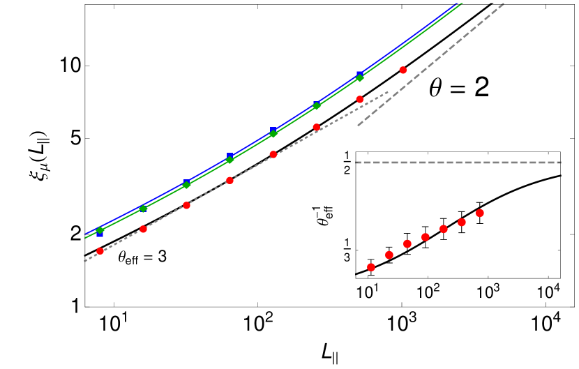
Figure 2: Perpendicular correlation lengths $\xi_{\mu}(L_{\parallel})$ for the $1{+}2\mathrm{d}$ geometry (red circles), the $2{+}1\mathrm{d}$ geometry in the $\perp_{1}$-direction (green diamonds) and in the $\perp_{2}$-direction (blue squares) at criticality. The statistical error is smaller than the symbol size. Due to corrections to scaling small systems have effective anisotropy exponent $\theta_{\mathrm{eff}}\approx 3$ (dotted line), which is obtained from the logarithmic derivative and shown exemplary for system $1{+}2\mathrm{d}$ in the inset.

We measured $G_{\perp}(L_{\parallel};r_{\mu})$ at criticality for both models using extensive Monte Carlo simulations and fitted the results against Eq. (20) to get $\xi_{\mu}(L_{\parallel})$ shown in Fig. 2. As in the 1+1d case we find corrections to scaling for $L_{\parallel}\lessapprox 300$ which are problematic in these three-dimensional cases as we cannot simulate systems larger than $L_{\parallel}=1024$. Hence we have to introduce a lattice correction term in the perpendicular correlation length and improve relation (9) using the ansatz

$$\xi_{\mu}(L_{\parallel})=A_{\mu}(L_{\parallel}+c_{0}L_{\parallel}^{1/2}+\ldots)^{1/\theta}$$ (21)

with $\theta=2$, which gives the best fit to the data. From the numerical data we find the amplitudes $A_{\mu}$ and $\hat{G}$ as well as the correction parameter $c_{0}$ listed in Tab. 1, and the resulting fit is shown as solid line in Fig. 2. For large systems the curve approaches the theoretical limit Eq. (9) with slope $\theta^{-1}=1/2$. Note that for small $L_{\parallel}\lesssim 64$ we could also find a reasonable data collapse with exponent $\theta_{\mathrm{eff}}=3$ (dotted line).

The resulting rescaled correlation functions for both models are presented in Fig. 3. In all cases the $y$-axis can be rescaled with $L_{\parallel}$ as predicted, without notable corrections. We find a convincing data collapse onto the mean-field correlation function $K_{0}(r/\xi)$ from Eq. (20). For small distances $r_{\perp_{2}}=\mathcal{O}(1)$ the correlation function $G_{\perp}(L_{\parallel};r_{\perp_{2}})$ differs from Eq. (20) due to the inplane nearest neighbor interactions.

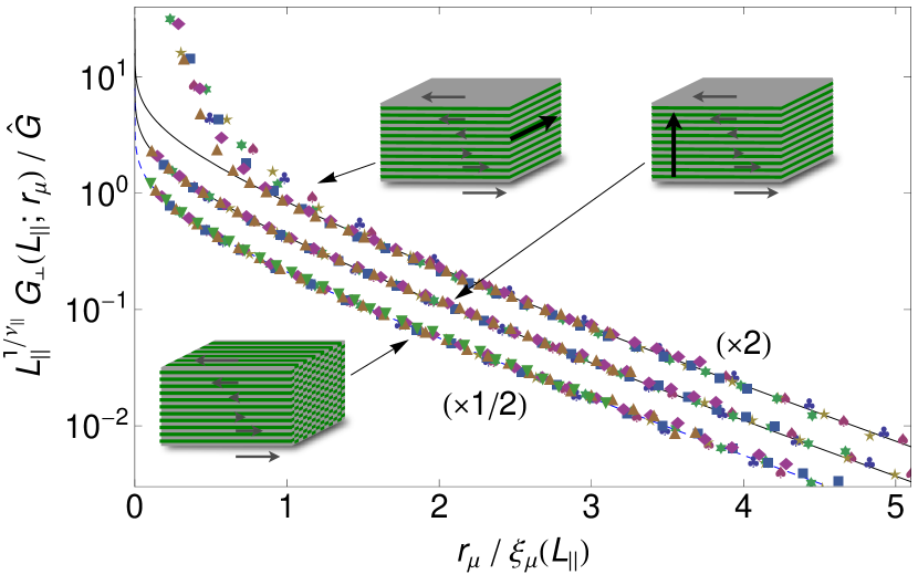
Figure 3: Rescaled correlation function $G_{\perp}(L_{\parallel};r_{\mu})$ with $\mu=\{\perp,\perp_{1},\perp_{2}\}$ for both models at criticality. We show varying system extensions $L_{\parallel}=\text{\{8,16,32,64,128,256,512,1024\}}$ for both cases. A rescaling of the $x$-axis with $\xi_{\mu}(L_{\parallel})$ and of the $y$-axis with $L_{\parallel}$ results in an excellent data collapse, verifying $\theta=2$ and $\nu_{\parallel}=1$. The solid lines represent the calculated Ornstein-Zernike correlation function, Eq. (20). Note that we multiplied the collapsed data with different factors as indicated in order to show them in one plot.

Now we comment on the four-dimensional geometry 1+3d, with decouples to a three-dimensional array of interacting chains, with $f=6$ in Eq. (2). We performed test simulations for system sizes up to $32^{3}\times 32$ and found very strong, possibly logarithmic corrections to scaling. From the scaling behavior of the available data we estimate that system sizes $L_{\parallel},L_{\perp}\gtrsim 1000$ would be required to find the correct scaling behavior.

Finally, we extend the dimensional analysis to the general case of a $d$-dimensional hyper-cubic sheared lattice with $d_{\parallel}$ driven dimensions and $d_{\perp}$ perpendicular dimensions. We again must distinguish between the $d_{\perp_{1}}$ dimensions normal to the shear and $d_{\perp_{2}}$ “inplane” dimensions without shear motion, with $d_{\perp}=d_{\perp_{1}}+d_{\perp_{2}}$. The critical temperature $T_{\mathrm{c}}$ at infinite shear velocity $v$ is given by Eq. (2), with the equilibrium zero field susceptibility $\chi_{\mathrm{eq}}^{(0)}$ of the $d_{\mathrm{eq}}$-dimensional system having $f$ fluctuating fields at each lattice point, where $d_{\mathrm{eq}}=d_{\parallel}+d_{\perp_{2}}$, and $f=2d_{\perp_{1}}$. From a simple generalization of Eq. (13) we find the exponents

$$\theta=\frac{4-d_{\perp}}{d_{\parallel}},\qquad\nu_{\parallel}=\frac{4-d_{\perp}}{2d_{\parallel}},\qquad\nu_{\perp}=\frac{1}{2},$$ (22)

fulfilling the hyperscaling relation $d_{\parallel}\nu_{\parallel}+d_{\perp}\nu_{\perp}=2$.

model		$\,d\,$	$d_{\parallel}$	$d_{\perp}$	$d_{\perp_{1}}$	$d_{\perp_{2}}$	$\theta$	$\nu_{\parallel}$	$f$	$d_{\mathrm{eq}}$	$T_{\mathrm{c}}(\infty)/J$
moved	1d	1	1	–	–	–	–	2	1	1	2.	2691853$\ldots$
	$2\mathrm{d}$	2	1	1	0	1	3	$\nicefrac{{3}}{{2}}$	1	2	4.	0587824$\ldots$
	$3\mathrm{d}$	3	1	2	0	2	2	1	1	3	5.	983835(1)
	$\textrm{2d}_{\mathrm{b}}$	1	1	–	–	–	–	2	1	2	2.	6614725$\ldots$
	$\textrm{3d}_{\mathrm{b}}$	2	1	1	0	1	3	$\nicefrac{{3}}{{2}}$	1	3	4.	8(1)
sheared	$1{+}1\mathrm{d}$	2	1	1	1	0	3	$\nicefrac{{3}}{{2}}$	2	1	3.	4659074$\ldots$
	$2{+}1\mathrm{d}$	3	1	2	1	1	2	1	2	2	5.	2647504$\ldots$
	$1{+}2\mathrm{d}$	3	1	2	2	0	2	1	4	1	5.	6426111$\ldots$
	$1{+}3\mathrm{d}$	4	1	3	3	0	1	$\nicefrac{{1}}{{2}}$	6	1	7.	728921$\ldots$
mix	$\mathrm{2\mathrm{d}}_{\mathrm{m}}$	2	2	–	–	–	–	1	1	1	4.	0587824$\ldots$
	$2{+}1\mathrm{d}_{\mathrm{m}}$	3	2	1	1	0	$\nicefrac{{3}}{{2}}$	$\nicefrac{{3}}{{4}}$	2	2	5.	2647504$\ldots$

Table 2: Relevant dimensions, exponents and parameters of the considered models, as defined in the text. For a classification see [9].

We conclude with a tabular summary of the found exponents and critical temperatures $T_{\mathrm{c}}$ at infinite driving velocity $v$ given in Table 2, including two cases denoted “mix” where we assumed a suitable two-dimensional motion of the interacting planes. These systems have $d_{\parallel}=2$, but notwithstanding the same $T_{\mathrm{c}}$ as the corresponding systems with unidirectional motion at infinite $v$. For the layered case $2{+}1\mathrm{d}_{\mathrm{m}}$ we predict the exponents $\theta=3/2$ and $\nu_{\parallel}=3/4$. A test of these predictions is left for future work.

7 Conclusion

We investigated the phase transition of three-dimensional Ising models with shear and two different shear normals by means of Monte Carlo simulations. In the limit of infinitely high shear velocity $v$ we found a critical temperature $T_{\mathrm{c}}(\infty)$ that depends on the direction of the shear normal. At criticality, strongly anisotropic diverging correlation lengths, with exponents $\nu_{\parallel}=1$ and $\nu_{\perp}=1/2$ occur, leading to an anisotropy exponent $\theta=2$, which confirms the results of a dimensional analysis of the corresponding Ginzburg-Landau-Wilson Hamiltonian. Furthermore, the dimensional analysis captures the anisotropy exponents as well as the correlation length exponents of the previously studied two-dimensional cases [12] and the parallel correlation length exponent of the one-dimensional cases [9]. Predictions for two-dimensional shear directions also result from the dimensional analysis, leading to the exponents $\theta=3/2$ and $\nu_{\parallel}=3/4$ in a three-dimensional model. Fluctuations perpendicular to the shear were shown to be Gaussian, resulting in a correlation function with Ornstein-Zernike behavior. Additionally, in the case of the $2{+}1\mathrm{d}$ geometry we found weakly anisotropic perpendicular correlations. As for $v=0$ the 2+1d and the 1+2d geometry reduce to the three-dimensional equilibrium Ising model, we expect a cross-over from this case to strongly anisotropic mean-field behavior similar to the $1{+}1\mathrm{d}$ geometry. In Ref. [12] an expensive analysis for finite velocities has been done leading to a crossover scaling, pointing out that all $v\neq 0$ provoke strongly anisotropic mean-field behavior, which is expected to occur in the current systems as well. However, we did not proof this in detail, due to the additional complexity in three-dimensional systems.