Braneworld non-minimal inflation with induced gravity

Abstract

We study cosmological inflation on a warped DGP braneworld where inflaton field is non-minimally coupled to induced gravity on the brane. We present a detailed calculation of the perturbations and inflation parameters both in Jordan and Einstein frame. We analyze the parameters space of the model fully to justify about the viability of the model in confrontation with recent observational data. We compare the results obtained in these two frames also in order to judge which frame gives more acceptable results in comparison with observational data.

PACS numbers

98.80.Cq,  98.80.-k,  04.50.-h

Key Words

Braneworld Inflation, Induced Gravity, Scalar-Tensor Gravity

I Introduction

Although the standard big bang cosmology has great successes in confrontation with observation, it suffers from some shortcomings such as the flatness, horizon and relics problems. It has been shown that an accelerating stage during the early time evolution of the universe with $\ddot{a}>0$ ($p<-\rho/3$) has the capability to solve these problems. This is the early time inflationary stage. The inflation also provides a mechanism for production of density perturbations needed to seed the formation of structures in the universe. It has been shown that a simple scalar field (usually dubbed inflaton) whose energy dominates the universe and whose potential energy dominates over the kinetic term (the slow-roll conditions) gives the required inflation Guth (1981); Linde (1982); Albrecht (1982); Linde (1990); Liddle (2000a); Lidsey (1997); Riotto (2002); Lyth (2009). Despite the great successes of the inflation paradigm, there are several problems with no concrete solutions: natural realization of inflation in a fundamental theory, cosmological constant and dark energy problem, unexpected low power spectrum at large scales and egregious running of the spectral index are some of these problems Brandenberger (2005). Another unsolved problem in the spirit of the inflationary scenario is that we don’t know how to integrate it with ideas of the particle physics. For example, we would like to identify the inflaton, the scalar field that drives inflation, with one of the known fields of particle physics. Also, it is important that the inflaton potential emerges naturally from underlying fundamental theory Lidsey (1997).

Braneworld scenarios open new windows to address at least part of these difficulties Lidsey (2004); Buchel (2004). One of the various braneworld scenarios, is the model proposed by Dvali, Gabadadze and Porrati (DGP). This setup is based on a modification of the gravitational theory in an induced gravity perspective Dvali (2000, 2001a, 2001b); Lue (2006). This induced gravity term in the brane part of the action, leads to deviations from the standard 4-dimensional gravity over large distances. In the DGP model, the bulk is a flat Minkowski spacetime, but a reduced gravity term appears on the brane without tension. Some aspects of the braneworld inflation in the pure DGP setup are studied in Lazkoz (2004); Corradini (2008). Maeda, Mizuno and Torii have constructed a braneworld scenario which combines the Randall-Sundrum II (RS II) Randall (1999) and DGP models Maeda (2003). In this combination, an induced curvature term appears on the brane in the RS II model. This model has been called the warped DGP braneworld in literatures Cai (2004); Zhang (2006); Nozari (2007a, 2011). Some aspects of the inflation on the warped DGP setup are studied in Refs. Cai (2004); Zhang (2006); Nozari (2007a, 2011).

We note that in a braneworld setup, the induced gravity on the brane arises as a result of quantum corrections. For instance, in the Randall-Sundrum II braneworld scenario quantum corrections arise due to induced coupling between brane matter and the bulk gravitons. The induced gravity leads to the appearance of terms proportional to the 4-dimensional Ricci scalar in the brane part of the action. While the RS model gives high-energy modifications to general relativity, the DGP braneworld produces a low energy modification that leads to late-time acceleration of brane universe even in the absence of dark energy. The RS II braneworld scenario modifies certainly the high energy, ultra-violet (UV) sector of the general relativity. Also the DGP gravity is essentially a low-energy, infra-red (IR) modification of the general relativity. Since the warped DGP scenario contains both UV and IR modifications simultaneously, inflation in a warped DGP setup is physically more reasonable than the pure RS II or DGP case. An important issue we are interested in this paper, is that whether high-energy inflation is subjected to the induced gravity effect. If the induced gravity correction takes the dominant role, then there is no RS-type high-energy regime in the early universe and we recover the DGP model. From another perspective, as the energy scale of inflation grows, the induced gravity correction acts to limit the growth of amplitude relative to the 4D case Langlois (2000, 2007); Bouhamdi-Lopez (2004); Kaloper (2005). Although induced gravity is an IR modification of General Relativity and it seems that these modifications have nothing to do with inflation, however the mentioned points are important enough to be the reason for study of the warped DGP-braneworld inflation. We note also that as has been shown in Lazkoz (2004), brane assisted inflation may be equally successful beyond general relativity. It has been proved that this is the case in the RS and DGP models provided certain conditions hold. Since we considered the normal branch of solutions, as has been shown in Lazkoz (2004) the conditions for the occurrence of inflation are less restrictive.

On the other hand, considering a braneworld setup has the advantage that bulk fields such as Radions (for stability purposes) can have projection(s) on the brane that is a suitable candidate for inflaton field on the brane. The projection of the bulk inflaton on the brane behaves just like an ordinary inflaton field in four dimensions in the low energy regime. While the origin of inflaton field in standard 4D case is not so trivial, in a braneworld picture we can imagine this field as a projection of bulk field(s). This may help to reduce at least part of lacuna of standard scenario. We note also that as has been shown in Buchel (2004), inflation in warped de Sitter string theory geometries bypasses the difficulties of computing corrections to $\eta$ slow-roll parameter relative to the effective four dimensional perspective.

Since inflaton can interact with other fields such as the gravitational sector of the theory, in the spirit of scalar-tensor theories, we can consider a non-minimal coupling (NMC) of the inflaton field with intrinsic (Ricci) curvature on the brane. Braneworld model with scalar field minimally or non-minimally coupled to gravity have been studied extensively (see Nozari (2007b) and references therein). We note that generally the introduction of the NMC is not just a matter of taste. The NMC is instead forced upon us in many situations of physical and cosmological interest. There are compelling reasons to include an explicit non-minimal coupling in the action. For instance, non-minimal coupling arises at the quantum level when quantum corrections to the scalar field theory are considered. Even if for the classical, unperturbed theory this non-minimal coupling vanishes, it is necessary for the renormalizability of the scalar field theory in curved space. In most theories used to describe inflationary scenarios, it turns out that a non-vanishing value of the coupling constant cannot be avoided Faraoni (1996, 2000, 1999); Spokoiny (1984); Futamase (1989); Salopek (1989); Fakir (1990); Schimd (2005); Makino (1991); Fakir (1992); Libanov (1998); Hwang (1999, 1998); Tsujikawa (1999a, b, 2000a); Chiba (2000); Tsujikawa (2000b); Gunzig (2001); Koh (2005); Marco (2006); Bojowald (2006); Bauer (2008); Easson (2009); Hertzberg (2010); Pallis (2010, 2011). Nevertheless, incorporation of an explicit non-minimal coupling has disadvantage that it is harder to realize inflation even with potentials that are known to be inflationary in the minimal theory Faraoni (1996, 2000, 1999). Using the conformal equivalence between gravity theories with minimally and non-minimally coupled scalar fields, for any inflationary model based on a minimally-coupled scalar field, it is possible to construct infinitely many conformally related models with a non-minimal coupling Spokoiny (1984); Futamase (1989); Salopek (1989); Fakir (1990); Schimd (2005); Makino (1991); Fakir (1992); Libanov (1998); Hwang (1999, 1998); Tsujikawa (1999a, b, 2000a); Chiba (2000); Tsujikawa (2000b); Gunzig (2001); Koh (2005); Marco (2006); Bojowald (2006); Bauer (2008); Easson (2009); Hertzberg (2010); Pallis (2010, 2011); Kaiser (1995); Chiba (2008). However, an important question then arises: are these conformally related frames really equivalent from physics viewpoint? This issue has been considered by several authors Capozziello (1997); Nandi (1998); Flanagan (2004); Bhadra (2007); Faraoni (2007); Nozari (2009); Capozziello (2010a, b); Quiros (2011a, b) and as a part of our primary goal, we are going to address this issue from a detailed comparison of the inflationary parameters in these two (Einstein and Jordan) frames.

Based on the mentioned preliminaries, in this paper we study cosmological inflation on a warped DGP braneworld where inflaton field is non-minimally coupled to induced gravity on the brane. We present a detailed calculation of the perturbations and inflation parameters both in Jordan and Einstein frame by adopting quadratic and quartic potentials. We analyze the parameter spaces of the models with details to have a comparison between two frames and also in order to constraint these models in confrontation with recent observational data.

II Braneworld inflation with induced gravity in Jordan frame

The action of a warped DGP model in which a single scalar field is non-minimally coupled to induced gravity on the brane can be written in the following form

$$S=\frac{1}{2\kappa_{5}^{2}}\int d^{5}x\sqrt{-g^{(5)}}\bigg{[}R^{(5)}-2\Lambda_{5}\bigg{]}+\int_{brane}d^{4}x\sqrt{-q}\bigg{[}\frac{1}{2\kappa_{4}^{2}}R+\frac{f(\varphi)}{2}\,R-\lambda-\frac{1}{2}q^{\mu\nu}\partial_{\mu}\varphi\partial_{\nu}\varphi-V(\varphi)\bigg{]}$$ (1)

where $\kappa_{5}^{2}$  is the five dimensional gravitational constant,  $R$  is the induced Ricci scalar on the brane,  $R^{(5)}$ is 5-dimensional Ricci scalar,  $\lambda$  is the brane tension and $\Lambda_{5}$ is the bulk cosmological constant. Also $q$ is the trace of the brane metric, $q_{\mu\nu}$. We remind that the mentioned action results in pure DGP model Dvali (2000, 2001a, 2001b) if $\lambda=0$ and $\Lambda_{5}=0$, and pure RSII model Randall (1999) if $\mu=0$ where $\mu$ is a mass scale which may correspond to the 4D Planck mass Maeda (2003). Also $f(\varphi)$ shows an explicit non-minimal coupling of the scalar field with induced gravity on the brane. We note that the fields and their interactions on the brane at the classical level will be determined by the bulk physics through boundary conditions on the brane. For instance, if $\Phi$ is assumed to be a bulk scalar field, as has been shown in Himemoto (2001, 2003); Yokoyama (2001); Sasaki (2004); Nozari (2012), the effective field on the brane will be $\varphi=\sqrt{r_{c}}\Phi$ and $V(\varphi)=\frac{r_{c}}{2}V(\frac{\Phi}{\sqrt{r_{c}}})$ through junction conditions on the brane. Also as we will show (see Eq. (6) below), $\Lambda_{5}=-\frac{\kappa_{5}^{4}}{6}\lambda^{2}\,$. So, these parameters cannot be freely adjusted and are influenced by bulk physics.

The generalized cosmological dynamics in this setup is given by the following Friedmann equation

$$H^{2}=\frac{\kappa_{4}^{2}}{3}\rho_{\varphi}+\frac{\kappa_{4}^{2}}{3}\lambda+\frac{2\kappa_{4}^{4}}{\kappa_{5}^{4}}\hskip 122.34692pt$$

$$\pm\frac{2\kappa_{4}^{2}}{\kappa_{5}^{2}}\,\sqrt{\frac{\kappa_{4}^{4}}{\kappa_{5}^{4}}+\frac{\kappa_{4}^{2}}{3}\rho_{\varphi}+\frac{\kappa_{4}^{2}}{3}\lambda-\frac{\Lambda_{5}}{6}-\frac{\mathcal{C}}{a^{4}}}.\hskip 14.22636pt$$ (2)

where $\rho_{\varphi}$ , the energy-density corresponding to the non-minimally coupled scalar field is defined as follows

$$\rho_{\varphi}=\frac{1}{2}\dot{\varphi}^{2}+V(\varphi)-6f^{\prime}(\varphi)H\dot{\varphi},$$ (3)

and the corresponding pressure is given by

$$p_{\varphi}=\frac{1}{2}\dot{\varphi}^{2}-V(\varphi)+2f^{\prime}(\varphi)\ddot{\varphi}+4f^{\prime}(\varphi)H\dot{\varphi}+2f^{\prime\prime}(\varphi)\dot{\varphi}^{2}.$$ (4)

We note that in this paper a prime represents the derivative with respect to the scalar field and a dot marks derivative with respect to the cosmic time. Now let’s to introduce the effective cosmological constant on the brane as

$$\Lambda_{eff}=\kappa_{4}^{2}\lambda+\frac{6\kappa_{4}^{4}}{\kappa_{5}^{4}}\pm\frac{\sqrt{6}\kappa_{4}^{4}}{\kappa_{5}^{4}}\sqrt{\Big{(}2\kappa_{4}^{2}\lambda-\Lambda_{5}\Big{)}\frac{\kappa_{5}^{4}}{\kappa_{4}^{4}}+6}\,.$$ (5)

Since we are interested in the inflationary dynamics driven by a scalar field with a self-interacting potential, we put the effective cosmological constant equal to zero. In this way, we find

$$\Lambda_{5}=-\frac{\kappa_{5}^{4}}{6}\lambda^{2}\,.$$ (6)

So, we can rewrite the Friedmann equation (2) as follows

$$H^{2}=\frac{\kappa_{4}^{2}}{3}\rho_{\varphi}+\frac{\kappa_{4}^{2}}{3}\lambda+\frac{2\kappa_{4}^{4}}{\kappa_{5}^{4}}\hskip 122.34692pt$$

$$\pm\frac{2\kappa_{4}^{2}}{\kappa_{5}^{2}}\,\sqrt{\frac{\kappa_{4}^{4}}{\kappa_{5}^{4}}+\frac{\kappa_{4}^{2}}{3}\rho_{\varphi}+\frac{\kappa_{4}^{2}}{3}\lambda-\frac{\kappa_{5}^{4}}{36}\lambda^{2}-\frac{\mathcal{C}}{a^{4}}}\,.\hskip 14.22636pt$$ (7)

Also, the second Friedmann equation is

$$\dot{H}=\frac{\kappa_{4}^{2}}{6H}\dot{\rho}_{\varphi}\pm\frac{\kappa_{4}^{2}}{\kappa_{5}^{2}}\frac{\frac{\kappa_{4}^{2}}{6H}\dot{\rho}_{\varphi}+\frac{2\mathcal{C}}{a^{4}}}{\sqrt{\frac{\kappa_{4}^{4}}{\kappa_{5}^{4}}+\frac{\kappa_{4}^{2}}{3}\rho_{\varphi}+\frac{\kappa_{4}^{2}}{3}\lambda-\frac{\kappa_{5}^{4}}{36}\lambda^{2}-\frac{\mathcal{C}}{a^{4}}}}\,\,.$$ (8)

Variation of the action (1) with respect to the scalar field gives the following equation of motion

$$\ddot{\varphi}+3H\dot{\varphi}-\frac{1}{2}f^{\prime}(\varphi)R+\frac{dV}{d\varphi}=0\,.$$ (9)

In the slow-roll approximation, where $\dot{\varphi}^{2}\ll V(\varphi)$ and $\ddot{\varphi}\ll|3H\dot{\varphi}|$, energy density and equation of motion for scalar field take the following forms respectively

$$\rho_{\varphi}\simeq V(\varphi)-6f^{\prime}(\varphi)H\dot{\varphi}\,,$$ (10)

$$3H\dot{\varphi}-\frac{1}{2}f^{\prime}(\varphi)R+\frac{dV}{d\varphi}\simeq 0\,.$$ (11)

Also, the Friedmann equation now takes the following form

$$H^{2}\simeq\frac{\kappa_{4}^{2}}{3}V-\frac{\kappa_{4}^{2}}{3}f^{\prime 2}R+\frac{2\kappa_{4}^{2}}{3}f^{\prime}V^{\prime}+\frac{\kappa_{4}^{2}}{3}\lambda+\frac{2\kappa_{4}^{4}}{\kappa_{5}^{4}}\pm\frac{2\kappa_{4}^{2}}{\kappa_{5}^{2}}\,\sqrt{\frac{\kappa_{4}^{4}}{\kappa_{5}^{4}}+\frac{\kappa_{4}^{2}}{3}V(\varphi)-\frac{\kappa_{4}^{2}}{3}f^{\prime 2}R+\frac{2\kappa_{4}^{2}}{3}f^{\prime}V^{\prime}+\frac{\kappa_{4}^{2}}{3}\lambda-\frac{\kappa_{5}^{4}}{36}\lambda^{2}-\frac{\mathcal{C}}{a^{4}}}\,.$$ (12)

Now, we define the slow-roll parameters as follows

$$\epsilon\equiv-\frac{\dot{H}}{H^{2}}\,\,,$$ (13)

$$\eta\equiv-\frac{1}{H}\frac{\ddot{H}}{\dot{H}}\,\,.$$ (14)

In the slow-roll approximation and by using equation (12) we find

$$\epsilon\simeq\frac{1}{2\kappa_{4}^{2}}\frac{V^{\prime 2}}{V^{2}}\times{\cal{A}}(\varphi)\,,$$ (15)

and

$$\eta\simeq\frac{1}{\kappa_{4}^{2}}\frac{V^{\prime\prime}}{V}\times{\cal{B}}(\varphi)\,,$$ (16)

where by definition

$${\cal{A}}(\varphi)=\Bigg{(}\frac{1}{V^{\prime}}-\frac{f^{\prime}R}{2V^{\prime 2}}\Bigg{)}\Bigg{(}V^{\prime}-2f^{\prime}f^{\prime\prime}R+2f^{\prime\prime}V^{\prime}+2f^{\prime}V^{\prime\prime}\Bigg{)}\hskip 213.39566pt$$

$$\times\frac{1\pm\frac{\kappa_{4}^{2}}{\kappa_{5}^{2}}\frac{1-\frac{\mathcal{C}}{a^{4}}\frac{36H^{2}}{\kappa_{4}^{2}\Big{(}V^{\prime}-\frac{f^{\prime}R}{2}\Big{)}\Big{(}V^{\prime}-2f^{\prime}f^{\prime\prime}R+2f^{\prime\prime}V^{\prime}+2f^{\prime}V^{\prime\prime}\Big{)}}}{\sqrt{\frac{\kappa_{4}^{4}}{\kappa_{5}^{4}}+\frac{\kappa_{4}^{2}}{3}V-\frac{\kappa_{4}^{2}}{3}f^{\prime 2}R+\frac{2\kappa_{4}^{2}}{3}f^{\prime}V^{\prime}+\frac{\kappa_{4}^{2}}{3}\lambda-\frac{\kappa_{5}^{4}}{36}\lambda^{2}-\frac{\mathcal{C}}{\hat{a}^{4}}}}}{\Bigg{[}1+\frac{\lambda}{V}-\frac{f^{\prime 2}R}{V}+\frac{2f^{\prime}V^{\prime}}{V}+\frac{6\kappa_{4}^{2}}{\kappa_{5}^{4}V}\pm\frac{6}{\kappa_{5}^{2}V}\,\sqrt{\frac{\kappa_{4}^{4}}{\kappa_{5}^{4}}+\frac{\kappa_{4}^{2}}{3}V-\frac{\kappa_{4}^{2}}{3}f^{\prime 2}R+\frac{2\kappa_{4}^{2}}{3}f^{\prime}V^{\prime}+\frac{\kappa_{4}^{2}}{3}\lambda-\frac{\kappa_{5}^{4}}{36}\lambda^{2}-\frac{\mathcal{C}}{a^{4}}}\,\,\Bigg{]}^{2}},$$ (17)

and

$${\cal{B}}(\varphi)=\Bigg{(}1-\frac{f^{\prime\prime}R}{2V^{\prime\prime}}\Bigg{)}\hskip 355.65944pt$$

$$\times\Bigg{\{}\frac{1}{1+\frac{\lambda}{V}-\frac{f^{\prime 2}R}{V}+\frac{2f^{\prime}V^{\prime}}{V}+\frac{6\kappa_{4}^{2}}{\kappa_{5}^{4}V}\pm\frac{6}{\kappa_{5}^{2}V}\,\sqrt{\frac{\kappa_{4}^{4}}{\kappa_{5}^{4}}+\frac{\kappa_{4}^{2}}{3}V-\frac{\kappa_{4}^{2}}{3}f^{\prime 2}R+\frac{2\kappa_{4}^{2}}{3}f^{\prime}V^{\prime}+\frac{\kappa_{4}^{2}}{3}\lambda-\frac{\kappa_{5}^{4}}{36}\lambda^{2}-\frac{\mathcal{C}}{a^{4}}}}\Bigg{\}}\,.$$ (18)

As we will show, these parameters which reflect the braneworld and non-minimal nature of our model, in the large field regime intensify the increment of the slow-roll parameters. Inflation can be attained only if $\{\epsilon,\eta\}<1$; once one of these parameters reaches unity, the inflation phase terminates. We note that ${\cal{A}}(\varphi)$ and ${\cal{B}}(\varphi)$ are contributions originating from braneworld nature of the setup and also the non-minimal coupling of the scalar field and induced gravity on the brane.

The number of e-folds during inflation is given by

$$N=\int_{t_{i}}^{t_{f}}Hdt\,,$$ (19)

which in the slow-roll approximation can be written as

$$N\simeq\int_{\varphi_{i}}^{\varphi_{f}}3H^{2}\frac{1}{\frac{1}{2}f^{\prime}R-V^{\prime}}d\varphi\,,$$ (20)

where $\varphi_{i}$ denotes the value of $\varphi$ when the universe scale observed today crosses the Hubble horizon during inflation and $\varphi_{f}$ is the value of $\varphi$ when the universe exits the inflationary phase. For a warped DGP model with non-minimally coupled scalar field on the brane, this quantity in Jordan frame becomes

$$N=\int_{\varphi_{hc}}^{\varphi_{f}}\Bigg{(}\frac{3V}{V^{\prime}}\Bigg{)}\Bigg{(}\frac{V^{\prime}}{\frac{1}{2}f^{\prime}R-V^{\prime}}\Bigg{)}\Bigg{[}\frac{\kappa_{4}^{2}}{3}+\frac{1}{V}\bigg{(}\frac{\kappa_{4}^{2}}{3}\lambda-\frac{\kappa_{4}^{2}f^{\prime 2}R}{3}+\frac{2\kappa_{4}^{2}f^{\prime}V^{\prime}}{3}+\frac{2\kappa_{4}^{4}}{\kappa_{5}^{4}}\hskip 142.26378pt$$

$$\pm\frac{2\kappa_{4}^{2}}{\kappa_{5}^{2}}\,\sqrt{\frac{\kappa_{4}^{4}}{\kappa_{5}^{4}}+\frac{\kappa_{4}^{2}}{3}V(\varphi)-\frac{\kappa_{4}^{2}}{3}f^{\prime 2}R+\frac{2\kappa_{4}^{2}}{3}f^{\prime}V^{\prime}+\frac{\kappa_{4}^{2}}{3}\lambda-\frac{\kappa_{5}^{4}}{36}\lambda^{2}-\frac{\mathcal{C}}{a^{4}}}\,\bigg{)}\Bigg{]}d\varphi\,\,.$$ (21)

After presentation of the main equations of the setup in Jordan frame, in the next section we consider the scalar perturbation of the metric since the key test of any inflation model is the spectrum of perturbations produced due to quantum fluctuations of the fields about their homogeneous background values.

III Perturbations in Jordan frame

In a warped DGP braneworld model, the effective covariant equations on the brane for an arbitrary brane metric and matter distribution is given by Maartens (2010)

$$G_{\mu\nu}=\kappa_{5}^{4}\Pi_{\mu\nu}-E_{\mu\nu}\,,$$ (22)

where

$$\Pi_{\mu\nu}=-\frac{1}{4}{\tau}_{\mu\sigma}{\tau}_{\nu}^{\sigma}+\frac{1}{12}{\tau}{\tau}_{\mu\nu}+\frac{1}{8}q_{\mu\nu}\Big{(}\tau_{\rho\sigma}{\tau}^{\rho\sigma}-\frac{1}{3}{\tau}^{2}\Big{)}\,.$$ (23)

$\tau_{\mu\nu}$ is the total stress-tensor on the brane and is defined as

$$\tau_{\,\,\nu}^{\mu}=-\kappa_{4}^{2}G_{\,\,\nu}^{\mu}-\lambda\delta_{\,\,\nu}^{\mu}+T_{\,\,\nu}^{\mu}\,,$$ (24)

where $T_{\mu\nu}$, the energy-momentum tensor of a scalar field non-minimally coupled to induced gravity on the brane is given by

$$T_{\mu\nu}=g_{\mu\nu}\Big{(}\frac{1}{2}fR-\frac{1}{2}g^{\alpha\beta}\partial_{\alpha}\varphi\,\partial_{\beta}\varphi-V(\varphi)\Big{)}+\partial_{\mu}\varphi\,\partial_{\nu}\varphi$$

$$-fR_{\mu\nu}-\Big{(}g_{\mu\nu}\Box-\nabla_{\mu}\nabla_{\nu}\Big{)}f\,.\hskip 71.13188pt$$ (25)

Also we have

$$E_{\mu\nu}=C_{MRS}^{\quad\quad N}\,\,n^{M}\,\,n_{N}\,\,{q^{R}}_{\mu}\,\,{q^{S}}_{\nu},$$ (26)

where $C_{MRS}^{\quad\quad N}$ is the five dimensional Weyl tensor and $n_{A}$ is the spacelike unit vector normal to the brane.

Depending on the choice of gauge (coordinates), there are many different ways of characterizing cosmological perturbations. In longitudinal gauge, the scalar metric perturbations of the FRW background are given by Bardeen (1980); Mukhanov (1992); Bertschinger (1995)

$$ds^{2}=-\big{(}1+2\Phi\big{)}dt^{2}+a^{2}(t)\big{(}1-2\Psi\big{)}\delta_{i\,j}\,dx^{i}dx^{j},$$ (27)

where $a(t)$ is the scale factor on the brane, $\Phi=\Phi(t,x)$ and $\Psi=\Psi(t,x)$ are the metric perturbations. For the above perturbed metric, one can obtain the perturbed field equations as follows

$$-3H(H\Phi+\dot{\Psi})-\frac{k^{2}}{a^{2}}=\frac{\kappa_{4}^{2}}{2}\delta\rho_{eff}\,,$$ (28)

$$\ddot{\Psi}+3H(H\Phi+\dot{\Psi})+H\dot{\Phi}+2\dot{H}\Phi+\frac{1}{3a^{2}}k^{2}(\Phi-\Psi)=\frac{\kappa_{4}^{2}}{2}\delta p_{eff}\,,$$ (29)

$$\dot{\Psi}+H\Phi=\frac{\kappa_{4}^{2}}{2}\Big{[}\frac{\kappa_{5}^{2}}{6\kappa_{4}^{2}}\rho_{\varphi}\dot{\varphi}\delta\varphi-\frac{\kappa_{5}^{2}}{6\kappa_{4}^{2}}\rho_{\varphi}\int(\delta T_{i}^{0})\,dx^{i}\Big{]}$$

$$+\frac{1}{2}\int(\delta E_{i}^{0})\,dx^{i}\,,\hskip 71.13188pt.$$ (30)

$$\Psi-\Phi=8\pi G\frac{\kappa_{4}^{2}H}{\kappa_{5}^{2}(\dot{H}+2H^{2})-H}a^{2}\delta\pi_{E}\,.$$ (31)

The anisotropic stress perturbation is defined as $\delta\pi_{ij}=[\partial_{i}\partial_{j}+(k^{2}/3)\delta_{ij}]\delta\pi$,   where $\pi$ is the trace of $\pi_{ij}$ . So, $\delta{\pi_{E}}$ is the anisotropic stress perturbation. In the Eqs. (28) and (29), $\rho_{eff}$ and $p_{eff}$ can be obtained from the standard Friedmann equation $H^{2}=\frac{\kappa_{4}^{2}}{3}\rho_{eff}$  as follows

$$\rho_{eff}=\rho_{\varphi}+\lambda+\frac{6\kappa_{4}^{2}}{\kappa_{5}^{4}}\hskip 142.26378pt$$

$$\pm\frac{6}{\kappa_{5}^{2}}\,\sqrt{\frac{\kappa_{4}^{4}}{\kappa_{5}^{4}}+\frac{\kappa_{4}^{2}}{3}\rho_{\varphi}+\frac{\kappa_{4}^{2}}{3}\lambda-\frac{\kappa_{5}^{4}}{36}\lambda^{2}-\frac{\mathcal{C}}{a^{4}}}\,\,.\hskip 28.45274pt$$ (32)

By using the continuity equation, $\dot{\rho}_{eff}+3H(\rho_{eff}+p_{eff})=0$, one can deduce

$$p_{eff}=p_{\varphi}\pm\frac{\kappa_{4}^{2}}{\kappa_{5}^{2}}\frac{\rho_{\varphi}+p_{\varphi}-\frac{4}{\kappa_{4}^{2}}\frac{\mathcal{C}}{a^{4}}}{\sqrt{\frac{\kappa_{4}^{4}}{\kappa_{5}^{4}}+\frac{\kappa_{4}^{2}}{3}\rho_{\varphi}+\frac{\kappa_{4}^{2}}{3}\lambda-\frac{\kappa_{5}^{4}}{36}\lambda^{2}-\frac{\mathcal{C}}{a^{4}}}}\hskip 28.45274pt$$

$$-\lambda-\frac{6\kappa_{4}^{2}}{\kappa_{5}^{4}}\mp\frac{6}{\kappa_{5}^{2}}\,\sqrt{\frac{\kappa_{4}^{4}}{\kappa_{5}^{4}}+\frac{\kappa_{4}^{2}}{3}\rho_{\varphi}+\frac{\kappa_{4}^{2}}{3}\lambda-\frac{\kappa_{5}^{4}}{36}\lambda^{2}-\frac{\mathcal{C}}{a^{4}}}\,.\hskip 18.49411pt$$ (33)

So, the perturbed effective density and pressure can be written as

$$\delta\rho_{eff}=\delta\rho_{\varphi}\pm\frac{\kappa_{4}^{2}}{\kappa_{5}^{2}}\,\frac{\delta\rho_{\varphi}-\frac{3}{\kappa_{4}^{2}}\delta E_{0}^{0}}{\sqrt{\frac{\kappa_{4}^{4}}{\kappa_{5}^{4}}+\frac{\kappa_{4}^{2}}{3}\rho_{\varphi}+\frac{\kappa_{4}^{2}}{3}\lambda-\frac{\kappa_{5}^{4}}{36}\lambda^{2}-E_{0}^{0}}}\,,$$ (34)

where $E_{0}^{0}=\frac{\mathcal{C}}{a^{4}}$ and

$$\delta p_{eff}=\delta p_{\varphi}\pm\frac{\kappa_{4}^{2}}{\kappa_{5}^{2}}\,\frac{\delta p_{\varphi}-\frac{1}{\kappa_{4}^{2}}\delta E_{0}^{0}}{\sqrt{\frac{\kappa_{4}^{4}}{\kappa_{5}^{4}}+\frac{\kappa_{4}^{2}}{3}\rho_{\varphi}+\frac{\kappa_{4}^{2}}{3}\lambda-\frac{\kappa_{5}^{4}}{36}\lambda^{2}-E_{0}^{0}}}\hskip 22.76228pt$$

$$-\lambda-\frac{6\kappa_{4}^{2}}{\kappa_{5}^{4}}\mp\frac{6}{\kappa_{5}^{2}}\,\sqrt{\frac{\kappa_{4}^{4}}{\kappa_{5}^{4}}+\frac{\kappa_{4}^{2}}{3}\rho_{\varphi}+\frac{\kappa_{4}^{2}}{3}\lambda-\frac{\kappa_{5}^{4}}{36}\lambda^{2}-\frac{\mathcal{C}}{a^{4}}}\,.\hskip 19.34766pt$$ (35)

$\delta E_{0}^{0}$ can be calculated from the general definition of $\delta E_{\nu}^{\mu}$ as

$$\delta E_{\,\nu}^{\mu}=-\kappa_{4}^{2}\left(\begin{array}[]{cc}-\delta\rho_{E}&a\delta q_{E}\\ a^{-1}\delta q_{E}&\frac{1}{3}\delta\rho_{E}\delta^{i}_{\,j}+(\delta\pi_{\,E})^{i}_{j}\\ \end{array}\right).$$ (36)

The (gauge-invariant) scalar perturbations of $E_{\,\nu}^{\mu}$ can be parameterized as an effective fluid with density perturbation $\delta\rho_{E}$, isotropic pressure perturbation $\frac{1}{3}\,\delta\rho_{E}$, anisotropic stress perturbation $\delta\pi_{E}$ and energy flux perturbation $\delta q_{E}$ (see Koyama (2006); Langlois (2001)). Also $\delta\rho_{\varphi}$ and $\delta p_{\varphi}$ take the following forms

$$\delta\rho_{\varphi}=\dot{\varphi}\delta\dot{\varphi}-\dot{\varphi}^{2}\Phi+V^{\prime}\delta\varphi+\delta\rho_{nmc},$$ (37)

where

$$\delta\rho_{nmc}=-2\Bigg{[}3H^{2}+\Big{(}\Box+\nabla_{0}\nabla^{0}\Big{)}f\Bigg{]}\Phi-6H^{2}f^{\prime}+f\delta R_{0}^{0}$$

$$-2\Bigg{[}\Box f-\frac{1}{2}fR\Bigg{]}\Phi-\Bigg{[}\Box+\nabla_{0}\nabla^{0}\Bigg{]}f^{\prime}\delta\varphi+\Bigg{[}\Big{(}\frac{k^{2}}{a^{2}}-3\dot{H}\Big{)}\Phi$$

$$-\frac{2k^{2}}{a^{2}}\Psi-3\Big{(}\ddot{\Psi}+4H\dot{\Psi}+H\dot{\Phi}+\dot{H}+4H^{2}\Phi\Big{)}\Bigg{]}f\,,\hskip 25.6073pt$$ (38)

and

$$\delta p_{\varphi}=\dot{\varphi}\delta\dot{\varphi}-\dot{\varphi}^{2}\Phi-V^{\prime}\delta\varphi+\delta p_{nmc}\,,$$ (39)

where

$$\delta p_{nmc}=-\frac{\delta^{i}_{j}}{3}\Bigg{\{}g^{jk}\Bigg{[}fR_{ki}-\big{(}g_{ki}\,\Box-\nabla_{k}\nabla_{i}\big{)}f\hskip 51.21504pt$$

$$-6g_{ki}\,f(\dot{H}+2H^{2})\Bigg{]}\Phi-g^{jk}\Bigg{[}f^{\prime}\Big{(}R_{ki}+6g_{ki}(\dot{H}+H^{2})\Big{)}\hskip 8.5359pt$$

$$-g_{ki}\,f\bigg{(}\Big{(}\frac{k^{2}}{a^{2}}-3\dot{H}\Big{)}\Phi-\frac{2k^{2}}{a^{2}}\Psi-3\Big{(}\ddot{\Psi}+4H\dot{\Psi}+H\dot{\Phi}\hskip 19.91684pt$$

$$+\dot{H}+4H^{2}\Phi\Big{)}\bigg{)}+f\,\delta R_{ki}+\Big{(}g_{ki}\Box-\nabla_{k}\nabla_{i}\Big{)}f^{\prime}\delta\varphi\hskip 28.45274pt$$

$$-\Big{(}\Box f-\frac{1}{2}f\Big{)}\delta g_{ki}\Bigg{]}\Bigg{\}}.\hskip 28.45274pt$$ (40)

Equations (37) and (39) in the minimal case and within the slow-roll conditions reduce to $\delta\rho_{\varphi}=\frac{dV}{d\varphi}\delta\varphi$ and $\delta p_{\varphi}=-\frac{dV}{d\varphi}\delta\varphi$  respectively. By perturbing the equation of motion of the scalar field (11), one obtains

$$\delta\ddot{\varphi}+3H\delta\dot{\varphi}+\Big{(}V^{\prime\prime}+\frac{k^{2}}{a^{2}}-\frac{1}{2}Rf^{\prime\prime}\Big{)}\delta\varphi=\dot{\varphi}\Big{(}3\dot{\Psi}+\dot{\Phi}\Big{)}$$

$$+\Phi\Big{(}Rf^{\prime}-2V^{\prime}\Big{)}+f^{\prime}\bigg{[}\Big{(}\frac{k^{2}}{a^{2}}-3\dot{H}\Big{)}\Phi-\frac{2k^{2}}{a^{2}}\Psi\hskip 28.45274pt$$

$$-3\Big{(}\ddot{\Psi}+4H\dot{\Psi}+H\dot{\Phi}+\dot{H}\Phi+4H^{2}\Phi\Big{)}\bigg{]}\,.\hskip 14.22636pt$$ (41)

Now the scalar perturbations can be decomposed to an entropy or isocurvature perturbation (the projection orthogonal to the trajectory), and adiabatic or curvature perturbations (projection parallel to the trajectory). The isocurvature perturbations are generated if inflation is driven by more than one scalar field Langlois (2000, 2007); Bassett (1999); Gordon (2001) or it interacts with other fields such as the induced gravity on the brane Bouhamdi-Lopez (2004); Kaloper (2005). The adiabatic perturbations are generated if the inflaton field is the only field in inflation period Bassett (1999); Gordon (2001); Bouhamdi-Lopez (2004); Kaloper (2005); Maartens (2000). Here, since the inflaton field is non-minimally coupled to the induced gravity on the brane, the entropy perturbations are presented in this setup Maartens (2000); Seahra (2010). A gauge-invariant primordial curvature perturbation $\zeta$, can be defined as follows Bardeen (1983)

$$\zeta=\Psi-\frac{H}{\dot{\rho}}\delta\rho\,\,.$$ (42)

This definition is valid to first order in the cosmological perturbations on scales outside the horizon. On uniform density hypersurfaces where $\delta\rho=0$, the above quantity reduces to the curvature perturbation, $\Psi$. In the warped DGP model and within the Jordan frame, we should redefine Eq. (42) as

$$\zeta=\Psi-\frac{H}{\dot{\rho}_{eff}}\delta\rho_{eff}\,\,.$$ (43)

Now, by using the energy conservation equation for linear perturbations (in an arbitrary gauge)

$$\dot{\delta\rho}_{eff}+3H(\delta\rho_{eff}+\delta p_{eff})+3(\rho_{eff}+p_{eff})\dot{\Psi}=0,$$ (44)

we can find the variation of $\zeta$ with respect to the conformal time as

$$\dot{\zeta}=\dot{\Psi}+\frac{\dot{\delta\rho}_{eff}}{3(\rho_{eff}+p_{eff})}-\frac{\dot{\rho}_{eff}+\dot{p}_{eff}}{3(\rho_{eff}+p_{eff})^{2}}\delta\rho_{eff}\,\,,$$ (45)

where $\dot{\rho}_{eff}$ and $\dot{p}_{eff}$ are given by time derivatives of equations (32) and (33) respectively.

One can split the pressure perturbation (in any gauge) into adiabatic and entropic (non-adiabatic) parts (see for instance Ref. Wands (2000))

$$\delta p_{eff}=c_{s}^{2}\delta\rho_{eff}+\dot{p}_{eff}\Gamma\,\,,$$ (46)

where $c_{s}^{2}=\frac{\dot{p}_{eff}}{\dot{\rho}_{eff}}$ is the sound effective velocity. The non-adiabatic part is $\delta p_{nad}=\dot{p}_{eff}\Gamma$ , where $\Gamma$ represents the displacement between hypersurfaces of uniform pressure and density. From equations (34)-(40) we can deduce

$$\delta p_{nad}=(1-c_{s}^{2})\delta\rho_{eff}-\Bigg{(}2V^{\prime}\delta\varphi+\delta\rho_{nmc}-\delta p_{nmc}\Bigg{)}\hskip 14.22636pt$$

$$\Bigg{(}1\pm\frac{\kappa_{4}^{2}}{\kappa_{5}^{2}}\frac{1}{\sqrt{\frac{\kappa_{4}^{4}}{\kappa_{5}^{4}}+\frac{\kappa_{4}^{2}}{3}\rho_{\varphi}+\frac{\kappa_{4}^{2}}{3}\lambda-\frac{\kappa_{5}^{4}}{36}\lambda^{2}-E_{0}^{0}}}\Bigg{)}\hskip 51.21504pt$$

$$\mp\frac{2\kappa_{4}^{2}}{\kappa_{5}^{2}}\frac{\frac{1}{\kappa_{4}^{2}}\delta E_{0}^{0}}{\sqrt{\frac{\kappa_{4}^{4}}{\kappa_{5}^{4}}+\frac{\kappa_{4}^{2}}{3}\rho_{\varphi}+\frac{\kappa_{4}^{2}}{3}\lambda-\frac{\kappa_{5}^{4}}{36}\lambda^{2}-E_{0}^{0}}}\hskip 68.28644pt$$

$$\mp\frac{\kappa_{4}^{4}}{6\kappa_{5}^{2}}\frac{\Big{(}\delta\rho_{\varphi}-\frac{1}{\kappa_{4}^{2}}\delta E_{0}^{0}\Big{)}\Big{(}\rho_{\varphi}+p_{\varphi}-\frac{4}{\kappa_{4}^{2}}E_{0}^{0}\Big{)}}{\Big{[}\frac{\kappa_{4}^{4}}{\kappa_{5}^{4}}+\frac{\kappa_{4}^{2}}{3}\rho_{\varphi}+\frac{\kappa_{4}^{2}}{3}\lambda-\frac{\kappa_{5}^{4}}{36}\lambda^{2}-E_{0}^{0}\Big{]}^{3/2}}\,.\hskip 28.45274pt$$ (47)

Using the equations (28)-(30) we can rewrite this relation as

$$\delta p_{nad}=-\frac{6}{\kappa_{4}^{2}}\bigg{(}1-c_{s}^{2}-{\cal{J}}\bigg{)}\frac{k}{a^{2}}\Psi\hskip 108.12054pt$$

$$-\frac{6}{\kappa_{4}^{2}}{\cal{K}}\bigg{(}H\Phi+\dot{\Psi}\bigg{)}+\frac{3}{\kappa_{4}^{2}}{\cal{J}}\delta E_{0}^{0}+\frac{2}{\kappa_{4}^{2}}\delta E_{0}^{0}\bigg{(}{\cal{I}}-1\bigg{)}\hskip 36.98866pt$$

$$+\Bigg{(}\delta p_{nmc}-\delta\rho_{nmc}-2\frac{V^{\prime}}{\dot{\varphi}}\int(\delta T_{i}^{0})_{nmc}\,dx^{i}\hskip 68.28644pt$$

$$+\frac{6\kappa_{4}^{2}}{\kappa_{5}^{2}}\frac{V^{\prime}}{\rho_{\varphi}\dot{\varphi}}\int\delta E_{i}^{0}\,dx^{i}\Bigg{)}{\cal{I}}\,,\hskip 51.21504pt$$ (48)

where ${\cal{K}}$,  ${\cal{J}}$ and ${\cal{I}}$ are defined as

$${\cal{K}}=\frac{6\kappa_{4}^{2}}{\kappa_{5}^{2}}\frac{V^{\prime}}{\rho_{\varphi}\dot{\varphi}}{\cal{I}}-3H{\cal{J}}\hskip 341.43306pt$$

$$+\frac{-3\bigg{(}2V^{\prime}\dot{\varphi}+\dot{\rho}_{nmc}-\dot{p}_{nmc}\bigg{)}{\cal{I}}+\frac{24}{\kappa_{4}^{2}}E_{0}^{0}H\bigg{(}{\cal{I}}-1\bigg{)}-3{\cal{J}}{\cal{I}}\bigg{(}\dot{\varphi}\ddot{\varphi}+V^{\prime}\dot{\varphi}+\dot{\rho}_{nmc}+\frac{12}{\kappa_{4}^{2}}E_{0}^{0}H\bigg{)}}{3\dot{\varphi}^{2}-\frac{1}{H}\bigg{(}\frac{1}{2}f^{\prime}\dot{\varphi}+\dot{\rho}_{nmc}\bigg{)}{\cal{I}}+\bigg{(}3\dot{\varphi}^{2}-\frac{12}{\kappa_{4}^{2}}E_{0}^{0}\bigg{)}\bigg{(}{\cal{I}}-1\bigg{)}}\,,$$ (49)

$${\cal{J}}=\frac{\kappa_{4}^{4}}{6\kappa_{5}^{4}}\frac{\Big{(}\rho_{\varphi}+p_{\varphi}-\frac{4}{\kappa_{4}^{2}}E_{0}^{0}\Big{)}}{\bigg{(}\frac{\kappa_{4}^{4}}{\kappa_{5}^{4}}+\frac{\kappa_{4}^{2}}{3}\rho_{\varphi}+\frac{\kappa_{4}^{2}}{3}\lambda-\frac{\kappa_{5}^{4}}{36}\lambda^{2}-E_{0}^{0}\bigg{)}^{3/2}\,{\cal{I}}}\,,$$ (50)

and

$${\cal{I}}=\Bigg{(}1\pm\frac{\kappa_{4}^{2}}{\kappa_{5}^{2}}\frac{1}{\sqrt{\frac{\kappa_{4}^{4}}{\kappa_{5}^{4}}+\frac{\kappa_{4}^{2}}{3}\rho_{\varphi}+\frac{\kappa_{4}^{2}}{3}\lambda-\frac{\kappa_{5}^{4}}{36}\lambda^{2}-E_{0}^{0}}}\Bigg{)}\,,$$ (51)

respectively. Now we can rewrite the equation governing on the variation of $\zeta$ versus the time in terms of the model’s parameters. From equations (44)-(48) we find

$$\dot{\zeta}=\frac{\kappa_{4}^{2}\rho_{eff}}{9H(\rho_{eff}+p_{eff})}\Bigg{(}\delta p_{nmc}-\delta\rho_{nmc}\hskip 96.73918pt$$

$$-\frac{2V^{\prime}}{\dot{\varphi}}\int(\delta T_{i}^{0})_{nmc}\,dx^{i}+\frac{6\kappa_{4}^{2}}{\kappa_{5}^{2}}\frac{V^{\prime}}{\rho_{\varphi}\dot{\varphi}}\int\delta E_{i}^{0}\,dx^{i}\Bigg{)}{\cal{I}}\hskip 56.9055pt$$

$$+\frac{\rho_{eff}\delta E_{0}^{0}}{3H(\rho_{eff}+p_{eff})}\Bigg{(}{\cal{J}}+\frac{2}{3}({\cal{I}}-1)\Bigg{)}\hskip 99.58464pt$$

$$-\frac{2(H\Phi+\dot{\Psi})}{3H(\rho_{eff}+p_{eff})}\rho_{eff}{\cal{K}}\hskip 96.73918pt$$ (52)

In the minimal case and within the standard model, the entropy perturbation vanishes for long wavelength; we have $\dot{\zeta}=0$ and the primordial spectrum of perturbation is due to adiabatic perturbations. But, it is obvious from equation (48) that in a DGP-inspired non-minimal setup, there is a non-vanishing contribution of the non-adiabatic perturbations, leading to non-vanishing $\dot{\zeta}$, which affects the primordial spectrum of perturbation. We note that isocurvature perturbations are free to evolve on superhorizon scales, and the amplitude at the present day depends on the details of the entire cosmological evolution from the time that they are formed. On the other hand, because all super-Hubble radius perturbations evolve in the same way, the shape of the isocurvature perturbation spectrum is preserved during this evolution Liddle (2000b); Cid (2007).

Here we are going to obtain scalar and tensorial perturbations in our model. We take into account the slow-roll approximation at the large scales, $k\ll aH$, where we need to describe the non-decreasing modes. Then by using the relation between Ricci scalar and $H$ and $\dot{H}$, we find from equation (41)

$$3H\delta\dot{\varphi}+\Big{(}V^{\prime\prime}-\frac{1}{2}f^{\prime\prime}R\Big{)}\delta\varphi\simeq\Phi\Big{(}2f^{\prime}R-2V^{\prime}\Big{)}\,.$$ (53)

We note that the reason for large scale assumption is that the scales of cosmological interest (e.g. for large-scale CMB anisotropies) have spent most of their time far outside the Hubble radius and have re-entered only relatively recently in the Universe history. In this respect, in the large scale the condition $k\ll aH$ is an acceptable assumption. As has been shown in Refs. Amendola (2006, 2007), when this condition is satisfied, $\dot{\Phi}$, $\dot{\Psi}$ and $\ddot{\Phi}$ can be neglected. In fact, for the longitudinal post-Newtonian limit to be satisfied, we require that $\Delta\Psi\gg a^{2}H^{2}\times(\Psi,\,\dot{\Psi},\,\ddot{\Psi})$, and similarly for other gradient terms Amendola (2006, 2007). For a plane wave perturbation with wavelength $\lambda$, we see that $H^{2}\Psi$ is much smaller than $\Delta\Psi$ when $\lambda\ll\frac{1}{H}$. The requirement that $\dot{\Psi}$ be also negligible implies the condition $\frac{d\log\Psi}{d\zeta}\ll\frac{1}{(\lambda H^{2})^{2}}$ (with $\zeta=\log a$), which holds if condition $\lambda\ll\frac{1}{H}$ is satisfied for perturbation growth. This argument can be applied for $\ddot{\Psi}$ and the other metric potential, $\Phi$ too. By adopting a similar reasoning, form Eq. (30) we have

$$\Phi\simeq\frac{\frac{\kappa_{5}^{2}}{6}\rho_{\varphi}+\frac{1}{\dot{\varphi}\delta\varphi}\int\delta E_{i}^{0}\,dx^{i}}{6H\bigg{(}1+\frac{\kappa_{5}^{2}}{18}\rho_{\varphi}f\bigg{)}}\dot{\varphi}\delta\varphi\,.$$ (54)

In writing the above equation we used the relation $\int(T_{i}^{0})_{nmc}\,dx^{i}=2f\Big{(}H\Phi+\dot{\Psi}\Big{)}$. By using equation (53) and (54), we can deduce

$$3H\delta\dot{\varphi}+\bigg{(}V^{\prime\prime}-\frac{1}{2}f^{\prime\prime}R\bigg{)}\delta\varphi\hskip 99.58464pt$$

$$\simeq\bigg{(}2f^{\prime}R-2V^{\prime}\bigg{)}\hskip 99.58464pt$$

$$\times\frac{\frac{\kappa_{5}^{2}}{6}\rho_{\varphi}+\frac{1}{\dot{\varphi}\delta\varphi}\int\delta E_{i}^{0}\,dx^{i}}{6H\left(1+\frac{\kappa_{5}^{2}}{18}\rho_{\varphi}f\right)}\dot{\varphi}\delta\varphi\,.\hskip 28.45274pt$$ (55)

By defining a function ${\cal{F}}$ as

$${\cal{F}}\equiv\frac{\delta\varphi}{V^{\prime}}\,,$$ (56)

equation (55) can be rewritten as

$$\frac{{\cal{F}}^{\prime}}{{\cal{F}}}=-\frac{\bigg{(}V^{\prime}-f^{\prime}R\bigg{)}\bigg{(}\frac{\kappa_{5}^{2}}{6}\rho_{\varphi}+\frac{1}{\dot{\varphi}\delta\varphi}\int\delta E_{i}^{0}\,dx^{i}\bigg{)}}{6\kappa_{4}^{2}\bigg{(}1+\frac{\kappa_{5}^{2}}{18}\rho_{\varphi}f\bigg{)}\bigg{(}\rho_{\varphi}+\lambda+\frac{6\kappa_{4}^{2}}{\kappa_{5}^{4}}\pm\frac{6}{\kappa_{5}^{2}}\,\sqrt{\frac{\kappa_{4}^{4}}{\kappa_{5}^{4}}+\frac{\kappa_{4}^{2}}{3}\rho_{\varphi}+\frac{\kappa_{4}^{2}}{3}\lambda-\frac{\kappa_{5}^{4}}{36}\lambda^{2}-\frac{\mathcal{C}}{a^{4}}}\bigg{)}}+\frac{\frac{1}{2}f^{\prime\prime}R-V^{\prime\prime}}{\frac{1}{2}f^{\prime}R-V^{\prime}}-\frac{V^{\prime\prime}}{V^{\prime}}\,.\hskip 56.9055pt$$ (57)

A solution of this equation is ${\cal{F}}={\cal{C}}\exp(\int\frac{{\cal{F}}^{\prime}}{{\cal{F}}}d\varphi)$, where ${\cal{C}}$ is an integration constant. So, from equation (56) we find

$$\delta\varphi={\cal{C}}\,V^{\prime}\exp\Bigg{[}-\int\Bigg{(}\frac{\Big{(}V^{\prime}-f^{\prime}R\Big{)}\Big{(}\frac{\kappa_{5}^{2}}{6}\rho_{\varphi}+\frac{1}{\dot{\varphi}\delta\varphi}\int\delta E_{i}^{0}\,dx^{i}\Big{)}}{6\kappa_{4}^{2}\Big{(}1+\frac{\kappa_{5}^{2}}{18}\rho_{\varphi}f\Big{)}\Big{(}\rho_{\varphi}+\lambda+\frac{6\kappa_{4}^{2}}{\kappa_{5}^{4}}\pm\frac{6}{\kappa_{5}^{2}}\,\sqrt{\frac{\kappa_{4}^{4}}{\kappa_{5}^{4}}+\frac{\kappa_{4}^{2}}{3}\rho_{\varphi}+\frac{\kappa_{4}^{2}}{3}\lambda-\frac{\kappa_{5}^{4}}{36}\lambda^{2}-\frac{\mathcal{C}}{a^{4}}}\Big{)}}\hskip 85.35826pt$$

$$+\frac{\frac{1}{2}f^{\prime\prime}R-V^{\prime\prime}}{\frac{1}{2}f^{\prime}R-V^{\prime}}-\frac{V^{\prime\prime}}{V^{\prime}}\Bigg{)}d\varphi\Bigg{]}\,.\hskip 28.45274pt$$ (58)

For simplicity we define the following quantity

$${\cal{G}}=\frac{-2\Big{(}V^{\prime}-\frac{1}{2}f^{\prime}R\Big{)}\Big{(}\frac{\kappa_{5}^{2}}{6}\rho_{\varphi}+\frac{1}{\dot{\varphi}\delta\varphi}\int\delta E_{i}^{0}\,dx^{i}\Big{)}}{6\Big{(}1+\frac{\kappa_{5}^{2}}{18}\rho_{\varphi}f\Big{)}\Big{(}\rho_{\varphi}+\lambda+\frac{6\kappa_{4}^{2}}{\kappa_{5}^{4}}\pm\frac{6}{\kappa_{5}^{2}}\,\sqrt{\frac{\kappa_{4}^{4}}{\kappa_{5}^{4}}+\frac{\kappa_{4}^{2}}{3}\rho_{\varphi}+\frac{\kappa_{4}^{2}}{3}\lambda-\frac{\kappa_{5}^{4}}{36}\lambda^{2}-\frac{\mathcal{C}}{a^{4}}}\Big{)}}-\frac{f^{\prime\prime}R-2V^{\prime\prime}}{\frac{1}{2}f^{\prime}R-V^{\prime}}+\frac{2V^{\prime\prime}}{V^{\prime}}.$$ (59)

As we have stated, brane parameters cannot be determined freely and are influenced by bulk physics through boundary conditions (see for instance Shtanov (2007) for details). In our case, the term $\frac{1}{\dot{\varphi}\delta\varphi}\int\delta E_{i}^{0}\,dx^{i}$ in Eqs. (58) and (59) which is a non-trivial contribution of the bulk on the brane is neglected in our forthcoming arguments. This means that we assume backreaction due to metric perturbations in the bulk can be neglected (we refer the reader to Maartens (2010); Hiramatsu (2006); Koyama (2007, 2008); Stewart (1993) for details and justification of this assumption). Based on the arguments provided in Maartens (2010), our assumption of neglecting the bulk-brane interactions in this study is viable. Now with definition (59), Eq. (58) can be rewritten as

$$\delta\varphi={\cal{C}}\,V^{\prime}\exp\bigg{(}\int{\cal{G}}d\varphi\bigg{)}\,.$$ (60)

So, the density perturbation is given by

$$A_{s}^{2}=\frac{k^{3}}{2\pi^{2}}\,\exp\bigg{(}2\int{\cal{G}}d\varphi\bigg{)}\,,$$ (61)

where the effects of the non-minimal coupling of the scalar field and induced gravity on the brane are hidden in the definition of ${\cal{G}}$. The scale-dependence of the perturbations is described by the spectral index as

$$n_{s}-1=\frac{d\ln A_{S}^{2}}{d\ln k}\,.$$ (62)

The interval in wave number is related to the number of e-folds by the relation

$$d\ln k(\varphi)=dN(\varphi)\,.$$

So we obtain

$$n_{s}=1-3\epsilon+\frac{2}{3}\eta\hskip 426.79134pt$$

$$+\Bigg{[}\frac{-2\Big{(}V^{\prime}-\frac{1}{2}f^{\prime}R\Big{)}\Big{(}\frac{\kappa_{5}^{2}}{6}\rho_{\varphi}\Big{)}}{6\Big{(}1+\frac{\kappa_{5}^{2}}{18}\rho_{\varphi}f\Big{)}\Big{(}\rho_{\varphi}+\lambda+\frac{6\kappa_{4}^{2}}{\kappa_{5}^{4}}\pm\frac{6}{\kappa_{5}^{2}}\,\sqrt{\frac{\kappa_{4}^{4}}{\kappa_{5}^{4}}+\frac{\kappa_{4}^{2}}{3}\rho_{\varphi}+\frac{\kappa_{4}^{2}}{3}\lambda-\frac{\kappa_{5}^{4}}{36}\lambda^{2}-\frac{\mathcal{C}}{a^{4}}}\Big{)}}\frac{9H^{2}}{\frac{1}{2}f^{\prime}R-V^{\prime}}+\frac{2V^{\prime\prime}}{V^{\prime}}\Bigg{]}\hskip 113.81102pt$$

$$\times\Bigg{[}\frac{\kappa_{4}^{2}}{3}+\frac{1}{V}\bigg{(}\frac{\kappa_{4}^{2}}{3}\lambda-\frac{\kappa_{4}^{2}f^{\prime 2}R}{3}+\frac{2\kappa_{4}^{2}f^{\prime}V^{\prime}}{3}+\frac{2\kappa_{4}^{4}}{\kappa_{5}^{4}}\hskip 284.52756pt$$

$$\pm\frac{2\kappa_{4}^{2}}{\kappa_{5}^{2}}\,\sqrt{\frac{\kappa_{4}^{4}}{\kappa_{5}^{4}}+\frac{\kappa_{4}^{2}}{3}V(\varphi)-\frac{\kappa_{4}^{2}}{3}f^{\prime 2}R+\frac{2\kappa_{4}^{2}}{3}f^{\prime}V^{\prime}+\frac{\kappa_{4}^{2}}{3}\lambda-\frac{\kappa_{5}^{4}}{36}\lambda^{2}-\frac{\mathcal{C}}{a^{4}}}\,\bigg{)}\Bigg{]}^{-1}\Bigg{(}\frac{V^{\prime}-\frac{1}{2}f^{\prime}R}{3V}\Bigg{)}.\hskip 31.2982pt$$ (63)

The running of the spectral index in our setup is given by

$$\alpha=\frac{dn_{s}}{d\ln k}\hskip 466.62502pt$$

$$=6\epsilon^{2}+2\epsilon\eta-\left[\frac{\frac{1}{2}f^{\prime\prime}R-V^{\prime\prime}}{H^{4}}\right]\left[V^{\prime\prime\prime}-\frac{1}{2}f^{\prime\prime\prime}R\right]+\frac{\frac{1}{2}\big{(}f^{\prime\prime}R-2V^{\prime\prime}\big{)}^{2}}{\big{(}\frac{1}{2}f^{\prime}R-V^{\prime}\big{)}^{2}}+\Bigg{[}\dot{H}+\frac{V^{\prime\prime}}{V^{\prime}}\bigg{(}\Big{(}V^{\prime\prime}-\frac{1}{2}f^{\prime\prime}R\Big{)}\Big{(}1+\frac{3H^{4}V^{\prime}}{2V^{\prime\prime}}\Big{)}+\dot{H}\bigg{)}\Bigg{]}\hskip 19.91684pt$$

$$\times\Bigg{[}\frac{-4\Big{(}V^{\prime}-\frac{1}{2}f^{\prime}R\Big{)}\Big{(}\frac{\kappa_{5}^{2}}{6}\rho_{\varphi}\Big{)}}{6\Big{(}1+\frac{\kappa_{5}^{2}}{18}\rho_{\varphi}f\Big{)}\Big{(}\rho_{\varphi}+\lambda+\frac{6\kappa_{4}^{2}}{\kappa_{5}^{4}}\pm\frac{6}{\kappa_{5}^{2}}\,\sqrt{\frac{\kappa_{4}^{4}}{\kappa_{5}^{4}}+\frac{\kappa_{4}^{2}}{3}\rho_{\varphi}+\frac{\kappa_{4}^{2}}{3}\lambda-\frac{\kappa_{5}^{4}}{36}\lambda^{2}-\frac{\mathcal{C}}{a^{4}}}\Big{)}}\Bigg{]}\left[\frac{V^{\prime}-\frac{1}{2}f^{\prime}R}{3H^{4}}\right]+{\cal{G}}^{\prime}+\frac{f^{\prime\prime\prime}R-2V^{\prime\prime\prime}}{\frac{1}{2}f^{\prime}R-V^{\prime}}-\frac{3\ddot{H}}{H^{2}}\hskip 14.22636pt$$

. (64)

The tensor perturbations amplitude of a given mode when leaving the Hubble radius are given by

$$A_{T}^{2}=\frac{4\kappa_{4}^{2}}{25\pi}H^{2}\Bigg{|}_{k=aH}\,.$$ (65)

In our setup and within the slow-roll approximation, we find

$$A_{T}^{2}=\frac{4\kappa_{4}^{2}}{25\pi}V\Bigg{[}\frac{\kappa_{4}^{2}}{3}+\frac{1}{V}\bigg{(}\frac{\kappa_{4}^{2}}{3}\lambda-\frac{\kappa_{4}^{2}f^{\prime 2}R}{3}+\frac{2\kappa_{4}^{2}f^{\prime}V^{\prime}}{3}+\frac{2\kappa_{4}^{4}}{\kappa_{5}^{4}}\hskip 256.0748pt$$

$$\hskip 113.81102pt\pm\frac{2\kappa_{4}^{2}}{\kappa_{5}^{2}}\,\sqrt{\frac{\kappa_{4}^{4}}{\kappa_{5}^{4}}+\frac{\kappa_{4}^{2}}{3}V(\varphi)-\frac{\kappa_{4}^{2}}{3}f^{\prime 2}R+\frac{2\kappa_{4}^{2}}{3}f^{\prime}V^{\prime}+\frac{\kappa_{4}^{2}}{3}\lambda-\frac{\kappa_{5}^{4}}{36}\lambda^{2}}\,\bigg{)}\Bigg{]}\,.\hskip 28.45274pt$$ (66)

The tensor spectral index is given by

$$n_{T}=\frac{d\ln A_{T}^{2}}{d\ln k}\,,$$ (67)

that in our model it takes the following form

$$n_{T}=\Bigg{(}\frac{V^{\prime}}{3V}\Bigg{)}\Bigg{(}\frac{f^{\prime}R-V^{\prime}}{V^{\prime}}\Bigg{)}\Bigg{[}\frac{\kappa_{4}^{2}}{3}+\frac{1}{V}\bigg{(}\frac{\kappa_{4}^{2}}{3}\lambda-\frac{\kappa_{4}^{2}f^{\prime 2}R}{3}+\frac{2\kappa_{4}^{2}f^{\prime}V^{\prime}}{3}+\frac{2\kappa_{4}^{4}}{\kappa_{5}^{4}}\hskip 170.71652pt$$

$$\hskip 96.73918pt\pm\frac{2\kappa_{4}^{2}}{\kappa_{5}^{2}}\,\sqrt{\frac{\kappa_{4}^{4}}{\kappa_{5}^{4}}+\frac{\kappa_{4}^{2}}{3}V(\varphi)-\frac{\kappa_{4}^{2}}{3}f^{\prime 2}R+\frac{2\kappa_{4}^{2}}{3}f^{\prime}V^{\prime}+\frac{\kappa_{4}^{2}}{3}\lambda-\frac{\kappa_{5}^{4}}{36}\lambda^{2}}\,\bigg{)}\Bigg{]}^{-1}\Sigma\,,\hskip 28.45274pt$$ (68)

where $\Sigma$ is defined as

$$\Sigma\equiv\frac{\kappa_{4}^{2}}{3}\bigg{(}\frac{V^{\prime}-2f^{\prime\prime}f^{\prime}R+2f^{\prime\prime}V^{\prime}+2f^{\prime}V^{\prime\prime}}{H^{2}}\bigg{)}\hskip 284.52756pt$$

$$\hskip 113.81102pt\times\bigg{(}1\pm\frac{{\kappa_{{4}}}^{2}}{{\kappa_{{5}}}^{2}}\frac{1}{\sqrt{{\frac{{\kappa_{{4}}}^{4}}{{\kappa_{{5}}}^{4}}}+\frac{\kappa_{4}^{2}}{3}V(\varphi)-\frac{\kappa_{4}^{2}}{3}f^{\prime 2}R+\frac{2\kappa_{4}^{2}}{3}f^{\prime}V^{\prime}+\frac{{\kappa_{{4}}}^{2}}{3}\lambda-\frac{\kappa_{5}^{4}}{36}\lambda^{2}}}\bigg{)}\,.\hskip 28.45274pt$$ (69)

In terms of the slow-roll parameters, the tensor (gravitational wave) spectral index can be expressed as

$$n_{T}=-2\epsilon\,.$$ (70)

The ratio between the amplitudes of tensor and scalar perturbations (tensor-to-scalar ratio) is given by

$$r\equiv\frac{A_{T}^{2}}{A_{S}^{2}}\simeq\frac{8\pi\kappa_{4}^{2}}{25}\frac{\exp\Bigg{(}\int-{\cal{G}}d\varphi\Bigg{)}}{{\cal{C}}^{2}V^{\prime 2}k^{3}}\,.$$ (71)

After a detailed calculation of the perturbations in Jordan frame, now we present an explicit example to see how previous equations work.

IV An explicit example: Monomial case with $f\sim\varphi^{2}$ and $V\sim\varphi^{2m}$

In this part, we take a monomial form of $f(\varphi)$ as

$$f(\varphi)=\xi\varphi^{2}\,,$$ (72)

where $\xi$ is a constant parameter. Also we choose the following form of the original scalar field potential in Jordan frame

$$V=\frac{b}{2m}\varphi^{2m}\,,$$ (73)

with constant $b$. In which follows, we intend to study two types of potentials: quadratic potential with $m=1$ and quartic potential with $m=2$. Further, we shall compare the outcomes of these two cases. By using equations (72) and (73) we rewrite the slow-roll parameters (Eqs.(13) and (14)) as

$$\epsilon=\left\{\begin{array}[]{ll}\frac{2}{\kappa_{4}^{2}}\left(\frac{b-\xi R}{b^{2}\varphi^{3}}\right)\left(b\varphi-8\xi^{2}\varphi R+8\xi b\varphi\right)\\ \times\frac{1\pm\frac{\kappa_{4}^{2}}{\kappa_{5}^{2}}\left(\sqrt{\frac{\kappa_{4}^{4}}{\kappa_{5}^{4}}+\frac{\kappa_{4}^{2}}{6}b\varphi^{2}+\frac{\kappa_{4}^{2}}{6}b\varphi^{2}-\frac{4\kappa_{4}^{2}}{3}\xi^{2}\varphi^{2}R+\frac{4\kappa_{4}^{2}}{3}\xi b\varphi^{2}+\frac{\kappa_{4}^{2}}{3}\lambda-\frac{\kappa_{5}^{4}}{36}\lambda^{2}}\right)^{-\frac{1}{2}}}{\left[1+\frac{2\lambda}{b\varphi^{2}}-\frac{8\xi^{2}R}{b}+8\xi+\frac{12\kappa_{4}^{2}}{\kappa_{5}^{4}b\varphi^{2}}\pm\frac{12}{\kappa_{5}^{2}b\varphi^{2}}\sqrt{\frac{\kappa_{4}^{4}}{\kappa_{5}^{4}}+\frac{\kappa_{4}^{2}}{6}b\varphi^{2}-+\frac{\kappa_{4}^{2}}{6}b\varphi^{2}-\frac{4\kappa_{4}^{2}}{3}\xi^{2}\varphi^{2}R+\frac{4\kappa_{4}^{2}}{3}\xi b\varphi^{2}+\frac{\kappa_{4}^{2}}{3}\lambda-\frac{\kappa_{5}^{4}}{36}\lambda^{2}}\right]^{2}}\quad\quad\quad m=1\vspace{0.5cm}\\ \\ \frac{8}{\kappa_{4}^{2}}\left(\frac{1}{b\varphi^{5}}-\frac{\xi R}{b^{2}\varphi^{7}}\right)\left(b\varphi^{3}-8\xi^{2}\varphi R+16\xi b\varphi^{3}\right)\\ \times\frac{1\pm\frac{\kappa_{4}^{2}}{\kappa_{5}^{2}}\left(\sqrt{\frac{\kappa_{4}^{4}}{\kappa_{5}^{4}}+\frac{\kappa_{4}^{2}}{12}b\varphi^{4}-\frac{4\kappa_{4}^{2}}{3}\xi^{2}\varphi^{2}R+\frac{4\kappa_{4}^{2}}{3}\xi b\varphi^{4}+\frac{\kappa_{4}^{2}}{3}\lambda-\frac{\kappa_{5}^{4}}{36}\lambda^{2}}\right)^{-\frac{1}{2}}}{\left[1+\frac{4\lambda}{b\varphi^{4}}-\frac{16\xi^{2}R}{b\varphi^{2}}+16\xi+\frac{24\kappa_{4}^{2}}{\kappa_{5}^{4}b\varphi^{4}}\pm\frac{24}{\kappa_{5}^{2}b\varphi^{4}}\sqrt{\frac{\kappa_{4}^{4}}{\kappa_{5}^{4}}+\frac{\kappa_{4}^{2}}{12}b\varphi^{4}-\frac{4\kappa_{4}^{2}}{3}\xi^{2}\varphi^{2}R+\frac{4\kappa_{4}^{2}}{3}\xi b\varphi^{4}+\frac{\kappa_{4}^{2}}{3}\lambda-\frac{\kappa_{5}^{4}}{36}\lambda^{2}}\right]^{2}},\quad\quad\quad\quad\quad\,m=2\vspace{0.5cm}\\ \end{array}\right.$$ (74)

and

$$\eta=\left\{\begin{array}[]{ll}\frac{2}{\kappa_{4}^{2}}\left(\frac{b-\xi R}{b\varphi^{2}}\right)\\ \times\frac{1}{\left[1+\frac{2\lambda}{b\varphi^{2}}-\frac{8\xi^{2}R}{b}+8\xi+\frac{12\kappa_{4}^{2}}{\kappa_{5}^{4}b\varphi^{2}}\pm\frac{12}{\kappa_{5}^{2}b\varphi^{2}}\sqrt{\frac{\kappa_{4}^{4}}{\kappa_{5}^{4}}+\frac{\kappa_{4}^{2}}{6}b\varphi^{2}-+\frac{\kappa_{4}^{2}}{6}b\varphi^{2}-\frac{4\kappa_{4}^{2}}{3}\xi^{2}\varphi^{2}R+\frac{4\kappa_{4}^{2}}{3}\xi b\varphi^{2}+\frac{\kappa_{4}^{2}}{3}\lambda-\frac{\kappa_{5}^{4}}{36}\lambda^{2}}\right]}\quad\,\,\quad m=1\vspace{0.5cm}\\ \\ \frac{12}{\kappa_{4}^{2}}\left(\frac{1}{\varphi^{2}}-\frac{\xi R}{3b\varphi^{4}}\right)\\ \times\frac{1}{\left[1+\frac{4\lambda}{b\varphi^{4}}-\frac{16\xi^{2}R}{b\varphi^{2}}+16\xi+\frac{24\kappa_{4}^{2}}{\kappa_{5}^{4}b\varphi^{4}}\pm\frac{24}{\kappa_{5}^{2}b\varphi^{4}}\sqrt{\frac{\kappa_{4}^{4}}{\kappa_{5}^{4}}+\frac{\kappa_{4}^{2}}{12}b\varphi^{4}-\frac{4\kappa_{4}^{2}}{3}\xi^{2}\varphi^{2}R+\frac{4\kappa_{4}^{2}}{3}\xi b\varphi^{4}+\frac{\kappa_{4}^{2}}{3}\lambda-\frac{\kappa_{5}^{4}}{36}\lambda^{2}}\right]}\quad\quad\quad\quad\quad m=2\vspace{0.5cm}\\ \end{array}\right.$$ (75)

Other inflation parameters such as $n_{S}$,  $n_{T}$ and $r$ can be expressed in terms of $\epsilon$ and $\eta$. We neglect presentation of these quantities here due to very lengthy structure of these equations. In which follows we perform an analysis on these parameters space.

IV.1 Quadratic Potential: $V(\varphi)=\frac{b}{2}\varphi^{2}$

The first inflaton potential we analyze is the quadratic potential, the case with $m=1$ in equation (73). The following figures are created as the outcome of our analysis of the model parameter space (we note that in all figures we have set $\kappa_{4}=\kappa_{5}=b=1$). Since $R=6(\dot{H}+2H^{2})$ and $H$ is nearly constant in the inflation epoch, we can consider in our numerical analysis $R$ to be approximately a constant and we set it to unity for simplicity. Nevertheless, we will consider a more general case by ignoring this assumption and adopting some reliable ansatz in our numerical analysis. We note also that all of our numerical analysis in this paper are performed for normal branch of this DGP-inspired model since this branch is ghost-free Koyama (2005); Izumi (2007); Koyama (2007); de Rham (2006). In the left panel of figure LABEL:fig:1, behavior of ${\cal{A}}(\varphi)$ as a correction factor to the standard result is depicted versus the scalar field. In this figure (and almost in all figures of this paper) we consider three values for $\xi$: $\frac{1}{12}$, $\frac{1}{8}$ and $\frac{1}{6}$. We note that $\xi=\frac{1}{6}$ is the conformal coupling of the standard general relativity Faraoni (1996, 2000, 1999); Fujii (2003).

The left panel of figure LABEL:fig:1 shows that as the scalar field decreases from the initial large values, ${\cal{A}}(\varphi)$ increases toward a maximum and then decreases. This maximum has different values for different $\xi$. As $\xi$ increases, the value of the maximum decreases and occurs in smaller values of the scalar field. Also, for each value of $\varphi$, the value of ${\cal{A}}(\varphi)$ decreases as $\xi$ increases. The behavior of ${\cal{A}}(\varphi)$ affects the behavior of the first slow-roll parameter $\epsilon$. This can be seen in the right panel of figure LABEL:fig:1. At large scalar field regime, the value of $\epsilon$ in warped DGP model is smaller than the corresponding value in the standard four dimensional model (here we note that in all of our figures the solid, black line curve represents the evolution of corresponding parameter in the standard 4D model). As the scalar field decreases, $\epsilon$ increases. For some value of the scalar field, $\epsilon$ takes the same value in both warped DGP and the standard four-dimensional model. For this value of the scalar field, ${\cal{A}}(\varphi)=1$. But, at some value of scalar field, $\epsilon$ reaches its maximum and then decreases. During this evolution, the behavior of $\epsilon$ in the warped DGP model is similar to the standard 4D case. With more reduction of the scalar field, $\epsilon$ deviates from 4D behavior and as the scalar field decreases, $\epsilon$ decreases similar to the correctional factor ${\cal{A}}(\varphi)$. This deviation from the 4D behavior is due to the presence of the brane tension. If there is no brane tension (also, with the zero effective cosmological constant), we attain the pure DGP model and the slow roll parameter always behaves as what it does in 4D model. In high energy regime, the effect of scalar field dominates the brane tension, but in low energy regime, where the scalar field becomes small, the brane tension’s effect becomes dominant in the dynamics of the model and so we can see the deviation of the standard 4D model. During the reduction of $\epsilon$, in some value of scalar field where ${\cal{A}}(\varphi)$ reaches to unity, the value of $\epsilon$ becomes equal to the 4D one again. We note that as for ${\cal{A}}(\varphi)$, the maximum value of $\epsilon$ depends on the value of $\xi$ too. As $\xi$ increases, the maximum becomes smaller and take places in smaller value of the scalar field. It means that for larger $\xi$, the 4D behavior lasts in wider domain of the scalar field values. For all values of $\xi$, it is possible for $\epsilon$ to reach unity and so the inflation has a graceful exit in this setup without need to any additional mechanism. In our setup, the slow-roll parameter reaches to unity twice. But, we know that the inflation occurs when ${\epsilon,\eta}\ll 1$. So, the first reaching of $\epsilon$ to unity, which take places in larger scalar field value, is the end of inflation since it reaches to unity from values smaller than $1$.
The behavior of the second correctional factor, ${\cal{B}}(\varphi)$, is more or less similar to ${\cal{A}}(\varphi)$. While the scalar field decreases, ${\cal{B}}$ increases to a maximum and then decreases (see the left panel of figure LABEL:fig:2). From the right panel of figure LABEL:fig:2, we can see the effect of the evolution of ${\cal{B}}$ on the second slow-roll parameter, $\eta$. $\eta$ in the warped DGP model always increases by reduction of the scalar field. This is similar to the behavior of $\eta$ in the standard four-dimensional case. However, due to the presence of the correctional factor ${\cal{B}}$, $\eta$ in the warped DGP model does not increase strictly as it does in 4D model (see the right panel of figure LABEL:fig:2). There is a maximum value for $\eta$ at $\varphi=0$. This maximum, for smaller $\xi$, has larger value. Since $\eta$ can attain the unit value too, the graceful exit from the inflationary phase in this model is guaranteed. We notify that in non-minimal inflation on the warped DGP brane within Jordan frame with a quadratic potential, both $\epsilon$ and $\eta$ are always positive. The next parameters that we consider are the scalar and tensorial spectral indices (shown as $n_{s}$ and $n_{T}$ respectively). In figures LABEL:fig:3 (the left panel) and  LABEL:fig:4, we have shown the behavior of the scalar and tensorial spectral indices versus the scalar field. One can realize the effect of first and second slow-roll parameters in the behavior of spectral indices. In the large values of the scalar field, both parameters behave similar to the corresponding parameters in the standard 4-dimensional model. It means that both scalar and spectral indices decrease by reduction of the scalar field strength. However, at some values of the scalar field, $n_{s}$ and $n_{T}$ reach a minimum and after that they increase, in contrast with the standard 4D case. The minimum value of these parameters decreases by reduction of $\xi$ and take places in larger values of the scalar field. So, for larger values of $\xi$, the standard behavior of $n_{s}$ and $n_{T}$ last in larger domain of $\varphi$ values. The general behavior of $n_{s}$ and $n_{T}$ is very similar to $\epsilon$ and $\eta$: similarity with the standard four-dimensional case in the large scalar field regime and deviation from it in the small scalar field regime.

Table 1: The values of some inflation parameters with a quadratic potential in Jordan frame at the time that physical scales crossed the horizon.

$\xi$	$n_{s}$	$r$	$\alpha$
$0$	$1.000000000$	$2.022875231\times 10^{-13}$	-3.029161336$\times 10^{-101}$
$\frac{1}{12}$	$0.9667051476$	$0.1575567389$	-1.670874757$\times 10^{-38}$
$\frac{1}{8}$	$0.9653928105$	$0.2094435340$	-2.537874469$\times 10^{-38}$
$\frac{1}{6}$	$0.9665654212$	$0.3137965930$	-3.269176612$\times 10^{-38}$
$observation$	$0.968\pm 0.012$	$<0.24(95\%CL)$	$-0.022\pm 0.020$

In the right panel of figure  LABEL:fig:3 we see the evolution of the running of the scalar spectral index, $\alpha$, versus the scalar field. In the large scalar field regime, the behavior of $\alpha$ is similar to the corresponding parameter in the standard 4D case and decreases by decreasing the scalar field value. But, at some value of the scalar field, $\alpha$ reaches its minimum value and then increases toward a maximum and after that, it decreases again. The minimum value of $\alpha$ take places in smaller scalar field values by increasing $\xi$. So, as $\xi$ increases, the 4D behavior of $\alpha$ lasts in larger domain of the scalar field. The last parameter that we are going to consider, is the ratio between the amplitudes of the tensor and scalar perturbations ($r$). We have shown the behavior of this ratio versus the scalar field in figure LABEL:fig:5. Its behavior is similar to the behavior of $\epsilon$ in general. As the scalar field decreases, $r$ increases toward a maximum in some values of the scalar field. Then, it begins to decrease. In other words, its evolution in the large scalar field region obeys the standard 4D behavior and in the small scalar field region, it evolves differently. Similar to other parameters, the extremum value of $r$ depends on the value of $\xi$. For larger $\xi$, the extremum value of $r$ becomes smaller and take places in smaller value of $\varphi$. So, for larger value of $\xi$, the ratio between the amplitudes of the tensor and scalar perturbations in warped DGP model, in larger domain of large $\varphi$, behaves as 4D model one.
Now we proceed to calculate some inflation parameters with a quadratic potential at the time that physical scales crossed the horizon. To find the value of the scalar field at the end of inflation, we set one of the slow-roll parameters, $\epsilon$ or $\eta$, equal to unity to get $\varphi_{f}$. To find the value of the scalar field at the time of horizon crossing, we have to adopt another strategy: the horizon crossing occurred about $60$ e-folds before the end of the inflation. So the definition of the number of e-folds helps us to find the value of the scalar field at the horizon crossing time, $\varphi_{hc}$. Now we rewrite the Friedmann equation (12) in the high energy limit ($\rho\gg\lambda$) as follows

$$H^{2}\simeq\Bigg{(}\frac{\kappa_{4}^{2}}{3}V-\frac{\kappa_{4}^{2}}{3}f^{\prime 2}R+\frac{2\kappa_{4}^{2}}{3}f^{\prime}V^{\prime}\Bigg{)}\hskip 76.82234pt$$

$$\times\Bigg{[}1-\frac{2\kappa_{4}^{2}}{\kappa_{5}^{2}}\Bigg{(}\frac{\kappa_{4}^{2}}{3}V-\frac{\kappa_{4}^{2}}{3}f^{\prime 2}R+\frac{2\kappa_{4}^{2}}{3}f^{\prime}V^{\prime}\Bigg{)}^{-\frac{1}{2}}\,\Bigg{]}.\hskip 17.07182pt$$ (76)

So, the number of e-folds by using equation (21) can be expressed as

$$N=3\int_{\varphi_{hc}}^{\varphi_{f}}\frac{\Big{(}\frac{\kappa_{4}^{2}}{3}V-\frac{\kappa_{4}^{2}}{3}f^{\prime 2}R+\frac{2\kappa_{4}^{2}}{3}f^{\prime}V^{\prime}\Big{)}}{\frac{1}{2}f^{\prime}R-V^{\prime}}\hskip 56.9055pt$$

$$\times\Bigg{[}1-\frac{2\kappa_{4}^{2}}{\kappa_{5}^{2}}\Bigg{(}\frac{\kappa_{4}^{2}}{3}V-\frac{\kappa_{4}^{2}}{3}f^{\prime 2}R+\frac{2\kappa_{4}^{2}}{3}f^{\prime}V^{\prime}\Bigg{)}^{-\frac{1}{2}}\,\Bigg{]}d\varphi\,.$$

We must solve the above integral in order to find $\varphi_{hc}$. In appendix A, we have presented the solution of the integral (77), where we assumed $\varphi_{hc}\gg\varphi_{f}$. Then we found $\varphi_{hc}$ from that solution and substitute it in the equations (63), (64) and (71) in order to find the values of these parameters at the time of the horizon crossing. Our analysis shows that although for all values of $0\leq\xi\leq\frac{1}{6}$, in the warped DGP model with a quadratic potential in Jordan frame we have $0.966\leq n_{s}\leq 1$ (so, the spectrum of the scalar perturbation is nearly scale invariant and red-tilted), but just for $\frac{1}{8}$ we arrive at $r\approx 0.22$  which is observationally more reliable Komatsu (2011). In this case the value of $r$ at the time of horizon crossing, decreases by decreasing $\xi$. Table 1 shows the value of the $n_{s}$, $r$ and $\alpha$ when the physical scales crossed the horizon for three different values of $\xi$. For comparison we have listed also the corresponding recently realized observational data. Note that the observational parameters are defined at $k_{0}=0.002$ Mpc^-1 where $k_{0}$ denotes the value of $k$ when universe scale crosses the Hubble horizon during inflation. Also these parameters are obtained via WMAP+BAO+H₀ Mean data, where Mean refers to the mean of the posterior distribution of each parameter. The quoted errors for $n_{s}$ show the $68\%$ confidence levels (CL) (see Komatsu (2011) for details). As the table shows, there is relatively good agreement between our results and recent observation. But note that the running of the spectral index in our setup is extra-ordinary close to zero. It is negative and in this respect viable. $n_{s}$ and $r$ are in good agreement with observation.

IV.2 Quartic Potential: $V(\varphi)=\frac{b}{4}\varphi^{4}$

The second potential we consider is the quartic potential i.e. the case with $m=2$ in equation (73). The left panel of figure LABEL:fig:6 shows the behavior of the correctional factor, ${\cal{A}}$ versus the scalar field in this case. In the large scalar field regime, ${\cal{A}}$ increases by reduction of the scalar field. So, in this situation $\epsilon$ increases and its behavior mimics the behavior of $\epsilon$ in the standard 4D case (see the right panel of figure LABEL:fig:6). However, the growth of ${\cal{A}}$ by reduction of the scalar field stopes at some value of the scalar field (which attains larger values for smaller $\xi$) and then it decreases. Similarly, by reduction of the scalar field $\epsilon$ reaches a maximum and its growth stopes. This maximum has larger value for smaller $\xi$. By further reduction of the scalar field, it deviates from the 4D behavior and decreases by reduction of the scalar field strength. In contrast with the quadratic potential where for small values of the scalar field the minimum of both ${\cal{A}}$ and $\epsilon$ were located at $\varphi_{min}=0$, here both ${\cal{A}}$ and $\epsilon$ have minimums located at some non-vanishing values of the scalar field. In fact, for quartic potential in this setup, $\epsilon$ has relatively more complicated structure than the quadratic case in the small scalar field regime. In the scale adopted in figure LABEL:fig:6, this behavior is not so evident, but it shall be more evident in figures of $n_{s}$ and $n_{T}$ versus the scalar field (as we will see later). Note that as $\xi$ increases, $\epsilon$ mimics the 4D behavior in a relatively wider domain of $\varphi$ values.

In the next step, we consider the evolution of the correctional factor ${\cal{B}}$ and the second slow-roll parameter $\eta$ versus $\varphi$ as shown in figure LABEL:fig:7. The general behavior of ${\cal{B}}$ and $\eta$ is similar to ${\cal{A}}$ and $\epsilon$. But, since the minimum value of these parameters occurs at $\varphi=0$, only in the large scalar field regime these parameters evolve similar to the corresponding parameters in 4D case. It should be noticed that for $\xi=\frac{1}{6}$ (the conformal coupling), the correctional factor ${\cal{B}}$ is always less than unity. It means that for this value of $\xi$, the value of $\eta$ in warped DGP model is always smaller than the value of this parameter in 4D model. We note also that in contrast with the quadratic potential case, the slow-roll parameters can be negative in some values of the scalar field.

In figures LABEL:fig:8 (the left panel) and LABEL:fig:9, we have shown the behavior of the scalar and tensor spectral index versus the scalar field. As we expected from the evolution of $\epsilon$, $n_{s}$ and $n_{T}$ at two extremal regimes of the scalar field evolve as they do in the standard four-dimensional model. At these two extremal regimes, $n_{s}$ and $n_{T}$ evolve from larger values to the smaller values by reduction of the scalar field. For other (intermediate) values of the scalar field, these parameters increase as the scalar field decreases. The behavior of the running of the scalar spectral index is shown in the right panel of figure LABEL:fig:8. In the large scalar field regime, $\alpha$ behaves as it does in 4D and decreases by reduction of the scalar field. This 4D behavior lasts in a wider domain of the scalar field for the larger values of $\xi$. But, at some value of the scalar field, $\alpha$ reaches its minimum and then increases to a maximum. After that, as scalar field decreases, there are other minimum and maximum values for $\alpha$, providing a relatively complicated structure relative to the quadratic potential case. This feature is shown in the right panel of the figure LABEL:fig:9 by adopting a smaller scale than the left panel one. Evidently there is a different structure of $n_{T}$ relative to the quadratic potential case where there was no minimum other than $\varphi_{min}=0$ in the small field regime.

Next we consider the tensor-to-scalar ratio, $r$. The result of this consideration is shown in figure LABEL:fig:10. For quartic potential, $r$ has more complicated behavior relative to the quadratic potential case in the small scalar field regime similar to the behavior of $\epsilon$, $n_{s}$ and $n_{T}$ in this regime. In two extremal regimes of the scalar field (large and small scalar field regimes), $r$ in the warped DGP model increases as the scalar field decreases. This is the same as the behavior of $r$ in the standard 4D case. For other (intermediate) values of the scalar field, it decreases by reduction of the scalar field.

Table 2: The values of some inflation parameters with a quartic potential in Jordan frame at the time that physical scales crossed the horizon.

$\xi$	$n_{s}$	$r$	$\alpha$
$0$	$0.9999999525$	$3.979559439\times 10^{-7}$	-6.534716905 $\times 10^{-58}$
$\frac{1}{12}$	$1.000000000$	$1.745217481\times 10^{-21}$	-1.238633640 $\times 10^{-51}$
$\frac{1}{8}$	$0.9999999999$	$1.137780227\times 10^{-21}$	-1.647520071 $\times 10^{-51}$
$\frac{1}{6}$	$0.9999999996$	$9.156848134\times 10^{-22}$	-8.485475908 $\times 10^{-51}$

Some inflation parameters calculated for quartic potential at the time that physical scales have crossed the horizon are shown in table 2. Similar to the quadratic potential case, the Friedmann equation and the number of e-folds are given via equations (76) and (77) but now with quartic potential. The solution of integral (77) with a quartic potential is presented in appendix B. By using that result and finding $\varphi_{hc}$ for this case, we obtain the values of the scalar spectral index, its running and the tensor to scalar ratio at the time of horizon crossing. The results for three values of $\xi$ is shown in table 2. We see that although for different values of $\xi$ the scalar spectral index is nearly scale invariant and red-tilted, the running of the spectral index and the tensor to scalar ratio increase by reduction of $\xi$. We note that the corresponding observational data and the conditions for calculations of these quantities are the same as what we have done for production of table 2.

Before presenting our analysis in the Einstein frame, we note that in our previous numerical analysis we argued that since $H$ is nearly constant in inflation epoch, the Ricci scalar $R=6(\dot{H}+2H^{2})$ is also nearly constant in this epoch. With this assumption, we have set $R=1$ in our numerical analysis. Now we consider a more general case to have more generic results: we consider the following ansatz for scale factor and scalar field

$$a(t)=a_{0}e^{\nu t},\,\quad\varphi=\varphi_{0}e^{-\vartheta t}$$

where $\nu$ and $\vartheta$ are positive constants. Note that these ansatz are chosen by taking into account the inflationary nature of the solutions for scale factor and a decreasing nature of the scalar field. Applying these ansatz to equation (11) and performing our numerical analysis for quadratic and quartic potentials with $\nu=10$, $a_{0}=\varphi_{0}=1$ and $\vartheta=1$, we find for $n_{s}$ the results that are shown in the left panel of figure LABEL:fig:5ab. These results are more generic than the case that we set the Ricci scalar to be a constant due to constancy of $H$ in inflation era. Also, the right panel of figure  LABEL:fig:5ab shows the results of our numerical calculation of the tensor-to-scalar ratio, $r$, for quadratic and quartic potentials adopting the above ansatz. Comparison of these more general results with the corresponding results obtained by a constant Ricci scalar shows that the results obtained by assumption of a constant Ricci scalar are actually reasonable in some sense. In fact, this comparison shows that the assumption of a constant Ricci scalar due to constancy of the Hubble parameter in inflation epoch is relatively a viable assumption. We have checked also the situation with ansatz

$$a(t)=\bigg{(}t^{2}+\frac{t_{0}}{1-\nu}\bigg{)}^{\frac{1}{1-\nu}},\,\quad\quad\varphi=\varphi_{0}t^{-\delta}$$

where we assume $\nu<1$,  $t_{0}>0$ (see for instance Cai (2007)) and $\delta>0$. Although this is not an exponentially solution of the scale factor, but the previous argument is applicable more or less even with this ansatz (for instance with $\nu=0.9$ and $\delta=3$). We note that the general case without adopting ansatz is far more difficult to find analytical or even numerical results.

V Inflation on the warped DGP brane in Einstein Frame

Up to now, we have considered the situation in Jordan frame. We can pass from Jordan to Einstein frame by making the following conformal transformation [22,24,41]

$$\hat{q}_{\mu\nu}=\Omega^{2}q_{\mu\nu}\,,$$ (78)

where the parameter $\Omega$ is defined as

$$\Omega^{2}=1+\kappa_{4}^{2}f(\varphi).$$ (79)

Under this transformation, action (1) in Einstein frame becomes

$$S=\frac{1}{2\kappa_{5}^{2}}\int d^{5}x\sqrt{-g^{(5)}}\Bigg{[}R^{(5)}-2\Lambda_{5}\Bigg{]}\hskip 341.43306pt$$

$$-\int d^{4}x\sqrt{-\hat{q}}\Bigg{[}\frac{1}{2\kappa_{4}^{2}}\,\hat{R}-\frac{3}{4}\left(\frac{\kappa_{4}^{2}f^{\prime}(\varphi)}{1+\kappa_{4}^{2}f(\varphi)}\right)^{2}\hat{q}^{\mu\nu}\partial_{\mu}\varphi\partial_{\nu}\varphi-\frac{1}{2}\Omega^{-4}\hat{q}^{\mu\nu}\partial_{\mu}\varphi\partial_{\nu}\varphi-\Omega^{-4}\lambda-\Omega^{-4}V(\varphi)\Bigg{]}.\hskip 28.45274pt$$ (80)

Now, we define a new scalar field $\hat{\varphi}$ in Einstein frame as follows

$$\frac{d\hat{\varphi}}{d\varphi}=\kappa_{4}^{-1}\sqrt{\frac{2(1+\kappa_{4}^{2}f(\varphi))+3\kappa_{4}^{2}f^{\prime 2}(\varphi)}{2(1+\kappa_{4}^{2}f(\varphi))^{2}}},$$ (81)

and the corresponding potential $\hat{V}$ defined in Einstein frame is

$$\hat{V}(\hat{\varphi})=\left[1+\kappa_{4}^{2}f(\varphi(\hat{\varphi}))\right]^{-2}V(\varphi(\hat{\varphi})).$$ (82)

The general condition for flatness of the potential at the large field limit is

$$\lim_{\varphi\rightarrow\infty}\frac{V}{f^{2}}=Const.>0.$$ (83)

The condition $f(\varphi)\gg\kappa_{4}^{-2}$ for $\varphi\gg\kappa_{4}^{-1}$ is required for the potential to be bounded from below and the location of the global minimum is well localized around the small field value. Even though the condition (83) actually determines the flatness of the potential at the large field limit, it is not necessarily required in generic inflation models. Depending on the shape of the potential, it might still be possible to have sufficient time of exponential expansion for some finite region of field value, $\varphi$ Park (2008).

The generalized cosmological dynamics of this setup in Einstein frame is given by the following Friedmann equation

$$\hat{H}^{2}=\frac{\kappa_{4}^{2}}{3}\rho_{\hat{\varphi}}+\frac{\kappa_{4}^{2}}{3}\hat{\lambda}+\frac{2\kappa_{4}^{4}}{\kappa_{5}^{4}}\hskip 113.81102pt$$

$$\pm\frac{2\kappa_{4}^{2}}{\kappa_{5}^{2}}\,\sqrt{\frac{\kappa_{4}^{4}}{\kappa_{5}^{4}}+\frac{\kappa_{4}^{2}}{3}\rho_{\hat{\varphi}}+\frac{\kappa_{4}^{2}}{3}\hat{\lambda}-\frac{\Lambda_{5}}{6}-\frac{\mathcal{C}}{\hat{a}^{4}}}.\hskip 14.22636pt$$ (84)

where  $\hat{}$   refers to parameters written in Einstein frame. In Friedmann equation (84) we defined $\hat{\lambda}=\frac{1}{(1+\kappa_{4}^{2}f(\varphi))^{2}}\lambda$ and $\hat{a}=(1+\kappa_{4}^{2}f(\varphi))^{1/2}a$. Also, $\rho_{\hat{\varphi}}$ the energy-density corresponding to the now minimally coupled scalar field in Einstein frame is defined as follows

$$\rho_{\hat{\varphi}}=\frac{1}{2}\left(\frac{d\hat{\varphi}}{d\hat{t}}\right)^{2}+\hat{V}(\hat{\varphi}),$$ (85)

and the corresponding pressure is given by

$$p_{\hat{\varphi}}=\frac{1}{2}\left(\frac{d\hat{\varphi}}{d\hat{t}}\right)^{2}-\hat{V}(\hat{\varphi}).$$ (86)

where $\hat{t}=(1+\kappa_{4}^{2}f(\varphi))^{1/2}t$ .

In this step, similar to the Jordan frame case, we introduce the effective cosmological constant on the brane in Einstein frame as follows

$$\hat{\Lambda}_{eff}=\kappa_{4}^{2}\hat{\lambda}+\frac{6\kappa_{4}^{4}}{\kappa_{5}^{4}}\pm\frac{\sqrt{6}\kappa_{4}^{4}}{\kappa_{5}^{4}}\sqrt{(2\kappa_{4}^{2}\hat{\lambda}-\Lambda_{5})\frac{\kappa_{5}^{4}}{\kappa_{4}^{4}}+6}\,.$$ (87)

By putting the effective cosmological constant equal to zero, we find

$$\Lambda_{5}=-\frac{\kappa_{5}^{4}}{6}\hat{\lambda}^{2}.$$ (88)

So, we can rewrite Friedmann equation (84) as follows

$$\hat{H}^{2}=\frac{\kappa_{4}^{2}}{3}\rho_{\hat{\varphi}}+\frac{\kappa_{4}^{2}}{3}\hat{\lambda}+\frac{2\kappa_{4}^{4}}{\kappa_{5}^{4}}\hskip 113.81102pt$$

$$\pm\frac{2\kappa_{4}^{2}}{\kappa_{5}^{2}}\,\sqrt{\frac{\kappa_{4}^{4}}{\kappa_{5}^{4}}+\frac{\kappa_{4}^{2}}{3}\rho_{\hat{\varphi}}+\frac{\kappa_{4}^{2}}{3}\hat{\lambda}-\frac{\kappa_{5}^{4}}{36}\hat{\lambda}^{2}-\frac{\mathcal{C}}{\hat{a}^{4}}}\,,\hskip 14.22636pt$$ (89)

and the second Friedmann equation can be expressed as

$$\frac{d\hat{H}}{d\hat{t}}=\frac{\kappa_{4}^{2}}{6\hat{H}}\frac{d\rho_{\hat{\varphi}}}{d\hat{t}}\pm\frac{\kappa_{4}^{2}}{\kappa_{5}^{2}}\frac{\frac{\kappa_{4}^{2}}{6\hat{H}}\frac{d\rho_{\hat{\varphi}}}{d\hat{t}}+\frac{\mathcal{C}}{\hat{a}^{4}}}{\sqrt{\frac{\kappa_{4}^{4}}{\kappa_{5}^{4}}+\frac{\kappa_{4}^{2}}{3}\rho_{\hat{\varphi}}+\frac{\kappa_{4}^{2}}{3}\hat{\lambda}-\frac{\kappa_{5}^{4}}{36}\hat{\lambda}^{2}-\frac{\mathcal{C}}{\hat{a}^{4}}}}\,\,.$$ (90)

The equation of motion of the scalar field in Einstein frame now is given by

$$\frac{d^{2}\hat{\varphi}}{d\hat{t}^{2}}+3\hat{H}\frac{d\hat{\varphi}}{d\hat{t}}+\frac{d\hat{V}}{d\hat{\varphi}}=0\,.$$ (91)

In the slow-roll approximation where $\left(\frac{d\hat{\varphi}}{d\hat{t}}\right)^{2}\ll\hat{V}(\hat{\varphi})$ and $\frac{d^{2}\hat{\varphi}}{d\hat{t}^{2}}\ll|3\hat{H}\frac{d\hat{\varphi}}{d\hat{t}}|$, energy density and equation of motion for the scalar field take the following forms respectively

$$\hat{\rho}\approx\hat{V}(\hat{\varphi})\,,$$ (92)

$$3\hat{H}\frac{d\hat{\varphi}}{d\hat{t}}+\frac{d\hat{V}}{d\hat{\varphi}}=0\,.$$ (93)

Now the Friedmann equation can be expressed as follows

$$\hat{H}^{2}=\frac{\kappa_{4}^{2}}{3}\hat{V}+\frac{\kappa_{4}^{2}}{3}\hat{\lambda}+\frac{2\kappa_{4}^{4}}{\kappa_{5}^{4}}\hskip 113.81102pt$$

$$\pm\frac{2\kappa_{4}^{2}}{\kappa_{5}^{2}}\,\sqrt{\frac{\kappa_{4}^{4}}{\kappa_{5}^{4}}+\frac{\kappa_{4}^{2}}{3}\hat{V}+\frac{\kappa_{4}^{2}}{3}\hat{\lambda}-\frac{\kappa_{5}^{4}}{36}\hat{\lambda}^{2}-\frac{\mathcal{C}}{\hat{a}^{4}}}\,\,.\hskip 14.22636pt$$ (94)

We define the slow-roll parameters in Einstein frame as

$$\hat{\epsilon}\equiv-\frac{1}{\hat{H}^{2}}\frac{d\hat{H}}{d\hat{t}},$$ (95)

$$\hat{\eta}\equiv-\frac{1}{\hat{H}}\frac{(d^{2}\hat{H})/(d\hat{t}^{2})}{(d\hat{H})/(d\hat{t})}\,.$$ (96)

In the slow-roll approximation, from Eq. (94) we find

$$\hat{\epsilon}=\frac{1}{2\kappa_{4}^{2}}\Bigg{(}\frac{(d\hat{V})/(d\hat{\varphi})}{\hat{V}}\Bigg{)}^{2}\left[\frac{1\pm\frac{\kappa_{4}^{2}}{\kappa_{5}^{2}}\bigg{(}1-\frac{36\hat{H}^{2}}{\kappa_{4}^{2}\left(\frac{d\hat{V}}{d\hat{\varphi}}\right)^{2}}\frac{\mathcal{C}}{\hat{a}^{4}}\bigg{)}\bigg{(}\sqrt{\frac{\kappa_{4}^{4}}{\kappa_{5}^{4}}+\frac{\kappa_{4}^{2}}{3}\hat{V}+\frac{\kappa_{4}^{2}}{3}\hat{\lambda}-\frac{\kappa_{5}^{4}}{36}\hat{\lambda}^{2}-\frac{\mathcal{C}}{\hat{a}^{4}}}\,\,\bigg{)}^{-\frac{1}{2}}}{\Bigg{(}1+\frac{1}{\hat{V}}\bigg{(}\hat{\lambda}+\frac{6\kappa_{4}^{2}}{\kappa_{5}^{4}}\pm\frac{6}{\kappa_{5}^{2}}\,\sqrt{\frac{\kappa_{4}^{4}}{\kappa_{5}^{4}}+\frac{\kappa_{4}^{2}}{3}\hat{V}+\frac{\kappa_{4}^{2}}{3}\hat{\lambda}-\frac{\kappa_{5}^{4}}{36}\hat{\lambda}^{2}-\frac{\mathcal{C}}{\hat{a}^{4}}}\bigg{)}\Bigg{)}^{2}}\right],$$ (97)

and

$$\hat{\eta}\simeq\frac{1}{\kappa_{4}^{2}}\Bigg{(}\frac{(d^{2}\hat{V})/(d\hat{\varphi}^{2})}{\hat{V}}\Bigg{)}\left[1+\frac{1}{\hat{V}}\Bigg{(}\hat{\lambda}+\frac{6\kappa_{4}^{2}}{\kappa_{5}^{4}}\pm\frac{6}{\kappa_{5}^{2}}\,\sqrt{\frac{\kappa_{4}^{4}}{\kappa_{5}^{4}}+\frac{\kappa_{4}^{2}}{3}\hat{V}+\frac{\kappa_{4}^{2}}{3}\hat{\lambda}-\frac{\kappa_{5}^{4}}{36}\hat{\lambda}^{2}-\frac{\mathcal{C}}{\hat{a}^{4}}}\Bigg{)}\right]^{-1}.$$ (98)

In equations (97) and (98), the terms in the brackets are corrections to the standard 4-dimensional model. These corrections are contributions originating from braneworld nature of the setup.

For warped DGP model with non-minimally coupled scalar field on the brane, the number of e-folds in Einstein frame becomes

$$\hat{N}=-\int_{\hat{\varphi}_{hc}}^{\hat{\varphi}_{f}}\Bigg{(}\frac{d\hat{\varphi}}{d\varphi}\Bigg{)}^{2}\Bigg{(}\frac{3\hat{V}}{d\hat{V}/d\varphi}\Bigg{)}\hskip 341.43306pt$$

$$\times\Bigg{[}\frac{\kappa_{4}^{2}}{3}+\frac{1}{\hat{V}}\bigg{(}\frac{\kappa_{4}^{2}}{3}\hat{\lambda}+\frac{2\kappa_{4}^{4}}{\kappa_{5}^{4}}\pm\frac{2\kappa_{4}^{2}}{\kappa_{5}^{2}}\,\sqrt{\frac{\kappa_{4}^{4}}{\kappa_{5}^{4}}+\frac{\kappa_{4}^{2}}{3}\hat{V}+\frac{\kappa_{4}^{2}}{3}\hat{\lambda}-\frac{\kappa_{5}^{4}}{36}\hat{\lambda}^{2}-\frac{\mathcal{C}}{\hat{a}^{4}}}\,\,\bigg{)}\Bigg{]}d\varphi\,\,.\hskip 28.45274pt$$ (99)

In the next section we consider the scalar perturbation of the metric in Einstein frame.

VI Perturbations in Einstein Frame

The effective covariant equations on the brane in a warped DGP braneworld scenario and in Einstein frame are given by

$$\hat{G}_{\mu\nu}=\kappa_{5}^{4}\hat{\Pi}_{\mu\nu}-\hat{E}_{\mu\nu},$$ (100)

where

$$\hat{\Pi}_{\mu\nu}=-\frac{1}{4}{\hat{\tau}}_{\mu\sigma}{\hat{\tau}}_{\nu}^{\sigma}+\frac{1}{12}{\hat{\tau}}{\hat{\tau}}_{\mu\nu}+\frac{1}{8}\hat{q}_{\mu\nu}\Big{(}{\hat{\tau}}_{\rho\sigma}{\hat{\tau}}^{\rho\sigma}-\frac{1}{3}{\hat{\tau}}^{2}\Big{)},$$ (101)

and $\hat{\tau}_{\mu\nu}$ is the total stress-tensor on the brane and is defined as

$$\hat{\tau}_{\,\,\nu}^{\mu}=-\kappa_{4}^{2}\hat{G}_{\,\,\nu}^{\mu}-\hat{\lambda}\delta_{\,\,\nu}^{\mu}+\hat{T}_{\,\,\nu}^{\mu}\,.$$ (102)

$\hat{T}_{\mu\nu}$, the energy-momentum tensor of the scalar field in Einstein frame which now is minimally coupled to the induced gravity on the brane, is given by (compare this result with corresponding equation in Jordan frame, Eq. (25))

$$\hat{T}_{\mu\nu}=\partial_{\mu}\hat{\varphi}\,\partial_{\nu}\hat{\varphi}-\hat{q}_{\mu\nu}\Big{(}\frac{1}{2}\hat{q}^{\alpha\beta}\partial_{\alpha}\hat{\varphi}\,\partial_{\beta}\hat{\varphi}+\hat{V}(\hat{\varphi})\Big{)}.$$ (103)

Also we have

$$\hat{E}_{\mu\nu}=C_{MRS}^{\quad\quad N}\,\,n^{M}\,\,n_{N}\,\,{\hat{q}^{R}}_{\mu}\,\,{\hat{q}^{S}}_{\nu}=\Omega^{4}E_{\mu\nu}$$ (104)

Since in Einstein frame $d\hat{s}^{2}=\Omega^{2}ds^{2}$, the scalar metric perturbations of the FRW background (Eq. (27)) is translated to

$$d\hat{s}^{2}=-\big{(}1+2\hat{\Phi}\big{)}d\hat{t}^{2}+\hat{a}^{2}(\hat{t})\big{(}1-2\hat{\Psi}\big{)}\delta_{i\,j}\,dx^{i}dx^{j}.$$ (105)

where $\hat{a}(\hat{t})$ is the scale factor on the brane in Einstein frame, $\hat{\Phi}=\hat{\Phi}(\hat{t},x)$ and $\hat{\Psi}=\hat{\Psi}(\hat{t},x)$ are the metric perturbations. For the above perturbed metric one can obtain the temporal part of the perturbed field equations in Einstein frame:

$$-3\hat{H}(\hat{H}\hat{\Phi}+\frac{d\hat{\Psi}}{d\hat{t}})-\frac{\hat{k}^{2}}{\hat{a}^{2}}=\frac{\kappa_{4}^{2}}{2}\delta\hat{\rho}_{eff}$$ (106)

$$\frac{d^{2}\hat{\Psi}}{d\hat{t}^{2}}+3\hat{H}(\hat{H}\hat{\Phi}+\frac{d\hat{\Psi}}{d\hat{t}})+\hat{H}\frac{d\Phi}{d\hat{t}}+2\frac{d\hat{H}}{d\hat{t}}\hat{\Phi}\hskip 56.9055pt$$

$$+\frac{1}{3\hat{a}^{2}}\hat{k}^{2}(\hat{\Phi}-\hat{\Psi})=\frac{\kappa_{4}^{2}}{2}\delta\hat{p}_{eff}\,,\hskip 22.76228pt$$ (107)

$$\frac{d\hat{\Psi}}{d\hat{t}}+\hat{H}\hat{\Phi}=\frac{\kappa_{4}^{2}}{2}\Big{(}\frac{\kappa_{5}^{4}\rho_{\hat{\varphi}}}{6\kappa_{4}^{2}}\frac{d\hat{\varphi}}{d\hat{t}}\delta\hat{\varphi}\Big{)}+\frac{1}{2}\int(\delta\hat{E}_{i}^{0})\,dx_{i}\,,$$ (108)

$$\hat{\Psi}-\hat{\Phi}=8\pi G\frac{\kappa_{4}^{2}\hat{H}}{\kappa_{5}^{2}(\frac{d\hat{H}}{d\hat{t}}+2\hat{H}^{2})-\hat{H}}\hat{a}^{2}\delta{\hat{\pi}_{\hat{E}}}\,.$$ (109)

In the last equation, $\delta{\hat{\pi}_{\hat{E}}}$ is anisotropic stress perturbation in the Einstein frame. In Eqs. (106) and (107), $\hat{\rho}_{eff}$ and $\hat{p}_{eff}$ can be obtained from the standard Friedmann equation $\hat{H}^{2}=\frac{\kappa_{4}^{2}}{3}\hat{\rho}_{eff}$, as follows

$$\hat{\rho}_{eff}=\rho_{\hat{\varphi}}+\hat{\lambda}+\frac{6\kappa_{4}^{2}}{\kappa_{5}^{4}}\hskip 139.41832pt$$

$$\pm\frac{6}{\kappa_{5}^{2}}\,\sqrt{\frac{\kappa_{4}^{4}}{\kappa_{5}^{4}}+\frac{\kappa_{4}^{2}}{3}\rho_{\hat{\varphi}}+\frac{\kappa_{4}^{2}}{3}\hat{\lambda}-\frac{\kappa_{5}^{4}}{36}\hat{\lambda}^{2}-\frac{\mathcal{C}}{\hat{a}^{4}}}.\hskip 22.76228pt$$ (110)

By using the continuity equation, $\frac{d}{d\hat{t}}\hat{\rho}_{eff}+3\hat{H}(\hat{\rho}_{eff}+\hat{p}_{eff})=0$, one can deduce

$$\hat{p}_{eff}=p_{\hat{\varphi}}\pm\frac{\kappa_{4}^{2}}{\kappa_{5}^{2}}\frac{\rho_{\hat{\varphi}}+p_{\hat{\varphi}}-\frac{4}{\kappa_{4}^{2}}\frac{\mathcal{C}}{\hat{a}^{4}}}{\sqrt{\frac{\kappa_{4}^{4}}{\kappa_{5}^{4}}+\frac{\kappa_{4}^{2}}{3}\rho_{\hat{\varphi}}+\frac{\kappa_{4}^{2}}{3}\hat{\lambda}-\frac{\kappa_{5}^{4}}{36}\hat{\lambda}^{2}-\frac{\mathcal{C}}{\hat{a}^{4}}}}-\hat{\lambda}\hskip 5.69046pt$$

$$-\frac{6\kappa_{4}^{2}}{\kappa_{5}^{4}}\mp\frac{6}{\kappa_{5}^{2}}\,\sqrt{\frac{\kappa_{4}^{4}}{\kappa_{5}^{4}}+\frac{\kappa_{4}^{2}}{3}\rho_{\hat{\varphi}}+\frac{\kappa_{4}^{2}}{3}\hat{\lambda}-\frac{\kappa_{5}^{4}}{36}\hat{\lambda}^{2}-\frac{\mathcal{C}}{\hat{a}^{4}}}\,.\hskip 19.91684pt$$ (111)

So, the perturbed effective density and pressure in Einstein frame can be written as

$$\delta\hat{\rho}_{eff}=\delta\rho_{\hat{\varphi}}\pm\frac{\kappa_{4}^{2}}{\kappa_{5}^{2}}\,\frac{\delta\rho_{\hat{\varphi}}-\frac{3}{\kappa_{4}^{2}}\delta\hat{E}_{0}^{0}}{\sqrt{\frac{\kappa_{4}^{4}}{\kappa_{5}^{4}}+\frac{\kappa_{4}^{2}}{3}\rho_{\hat{\varphi}}+\frac{\kappa_{4}^{2}}{3}\hat{\lambda}-\frac{\kappa_{5}^{4}}{36}\hat{\lambda}^{2}-\hat{E}_{0}^{0}}}.$$ (112)

and

$$\delta\hat{p}_{eff}=\delta p_{\hat{\varphi}}\pm\frac{6}{\kappa_{5}^{2}}\,\frac{\delta p_{\hat{\varphi}}-\frac{1}{\kappa_{4}^{2}}\delta\hat{E}_{0}^{0}}{\sqrt{\frac{\kappa_{4}^{4}}{\kappa_{5}^{4}}+\frac{\kappa_{4}^{2}}{3}\rho_{\hat{\varphi}}+\frac{\kappa_{4}^{2}}{3}\hat{\lambda}-\frac{\kappa_{5}^{4}}{36}\hat{\lambda}^{2}-\hat{E}_{0}^{0}}}\hskip 5.69046pt$$

$$\mp\frac{\kappa_{4}^{4}}{6\kappa_{5}^{2}}\frac{\Big{(}\delta\rho_{\hat{\varphi}}-\frac{1}{\kappa_{4}^{2}}\delta\hat{E}_{0}^{0}\Big{)}\Big{(}\rho_{\hat{\varphi}}+\hat{p}-\frac{4}{\kappa_{4}^{2}}\hat{E}_{0}^{0}\Big{)}}{\Big{[}\frac{\kappa_{4}^{4}}{\kappa_{5}^{4}}+\frac{\kappa_{4}^{2}}{3}\rho_{\hat{\varphi}}+\frac{\kappa_{4}^{2}}{3}\hat{\lambda}-\frac{\kappa_{5}^{4}}{36}\hat{\lambda}^{2}-\hat{E}_{0}^{0}\Big{]}^{3/2}}\,,\hskip 19.91684pt$$ (113)

where $\delta\hat{E}_{0}^{0}$ can be calculated from the following relation

$$\delta\hat{E}_{\,\nu}^{\mu}=-\kappa_{4}^{2}\left(\begin{array}[]{cc}-\delta\hat{\rho}_{\hat{E}}&a\delta\hat{q}_{\hat{E}}\\ \hat{a}^{-1}\delta\hat{q}_{\hat{E}}&\frac{1}{3}\delta\hat{\rho}_{\hat{E}}\delta^{i}_{\,j}+(\delta\hat{\pi}_{\,\hat{E}})^{i}_{j}\\ \end{array}\right)\,,$$ (114)

that is written in Einstein frame. Also $\delta\rho_{\hat{\varphi}}$ and $\delta p_{\hat{\varphi}}$ take the following forms

$$\delta\rho_{\hat{\varphi}}=\frac{d\hat{\varphi}}{d\hat{t}}\,\,\delta\left(\frac{d\hat{\varphi}}{d\hat{t}}\right)-\left(\frac{d\hat{\varphi}}{d\hat{t}}\right)^{2}\hat{\Phi}+\frac{d\hat{V}}{d\hat{\varphi}}\delta\hat{\varphi},$$ (115)

$$\delta p_{\hat{\varphi}}=\frac{d\hat{\varphi}}{d\hat{t}}\,\,\delta\left(\frac{d\hat{\varphi}}{d\hat{t}}\right)-\left(\frac{d\hat{\varphi}}{d\hat{t}}\right)^{2}\hat{\Phi}-\frac{d\hat{V}}{d\hat{\varphi}}\delta\hat{\varphi}.$$ (116)

These equations in the slow-roll regime reduce to $\delta\rho_{\hat{\varphi}}=\frac{d\hat{V}}{d\hat{\varphi}}\delta\hat{\varphi}$ and $\delta p_{\hat{\varphi}}=-\frac{d\hat{V}}{d\hat{\varphi}}\delta\hat{\varphi}$  respectively. By perturbing the equation of motion of the scalar field (91) one can find

$$\delta\frac{d^{2}\hat{\varphi}}{d\hat{t}^{2}}+3\hat{H}\delta\left(\frac{d\hat{\varphi}}{d\hat{t}}\right)+\left(\frac{d^{2}\hat{V}}{d\hat{\varphi}^{2}}+\frac{\hat{k}^{2}}{\hat{a}^{2}}\right)\delta\hat{\varphi}\hskip 56.9055pt$$

$$=\frac{d\hat{\varphi}}{d\hat{t}}\left(3\frac{d\hat{\Psi}}{d\hat{t}}+\frac{d\hat{\Phi}}{d\hat{t}}\right)+\hat{\Phi}\left(-2\frac{d\hat{V}}{d\hat{\varphi}}\right).\hskip 25.6073pt$$ (117)

In Einstein frame and within the warped DGP model, we should redefine equation (43) as

$$\hat{\zeta}=\hat{\Psi}-\frac{\hat{H}}{(d\hat{\rho}_{eff})/(d\hat{t})}\delta\hat{\rho}_{eff}.$$ (118)

where $\hat{\Psi}$ is an Einstein frame quantity. Now, by using the energy-conservation equation for linear perturbations,

$$\frac{d}{d\hat{t}}\delta\hat{\rho}_{eff}+3\hat{H}(\delta\hat{\rho}_{eff}+\delta\hat{p}_{eff})+3(\hat{\rho}_{eff}+\hat{p}_{eff})\frac{d\hat{\Psi}}{d\hat{t}}=0,$$ (119)

we find the variation of $\hat{\zeta}$ with respect to the conformal time as

$$\frac{d\hat{\zeta}}{d\hat{t}}=\frac{d\hat{\Psi}}{d\hat{t}}+\frac{\frac{d}{d\hat{t}}\delta\hat{\rho}_{eff}}{3(\hat{\rho}_{eff}+\hat{p}_{eff})}-\frac{\frac{d}{d\hat{t}}(\hat{\rho}_{eff}+\hat{p}_{eff})}{(\hat{\rho}_{eff}+\hat{p}_{eff})^{2}}\delta\hat{\rho}_{eff},$$ (120)

where $\frac{d\hat{\rho}_{eff}}{d\hat{t}}$ and $\frac{d\hat{p}_{eff}}{d\hat{t}}$ are given by time derivatives of equations (110) and (111) respectively.

Similar to the Jordan frame case, we split the pressure perturbations into adiabatic and entropic parts as follows

$$\delta\hat{p}_{eff}=c_{s}^{2}\delta\hat{\rho}_{eff}+\frac{d\hat{p}_{eff}}{d\hat{t}}\hat{\Gamma}\,.$$ (121)

The non-adiabatic part is $\delta p_{nad}=\frac{d\hat{p}_{eff}}{d\hat{t}}\hat{\Gamma}$ , where $\hat{\Gamma}$ is defined as

$$\hat{\Gamma}=\frac{\delta\hat{p}_{eff}}{(d\hat{p}_{eff})/(d\hat{t})}-\frac{\delta\hat{\rho}_{eff}}{(d\hat{\rho}_{eff})/(d\hat{t})}.$$ (122)

From Equations (112)-(116) we can deduce

$$\delta\hat{p}_{nad}=\Bigg{(}1-\hat{c}_{s}^{2}\Bigg{)}\delta\hat{\rho}_{eff}-\Bigg{(}2\frac{d\hat{V}}{d\hat{\varphi}}\delta\hat{\varphi}\Bigg{)}\Bigg{(}1\pm\frac{\kappa_{4}^{2}}{\kappa_{5}^{2}}\frac{1}{\sqrt{\frac{\kappa_{4}^{4}}{\kappa_{5}^{4}}+\frac{\kappa_{4}^{2}}{3}\rho_{\hat{\varphi}}+\frac{\kappa_{4}^{2}}{3}\hat{\lambda}-\frac{\kappa_{5}^{4}}{36}\hat{\lambda}^{2}-\hat{E}_{0}^{0}}}\Bigg{)}\hskip 142.26378pt$$

$$\mp\frac{2\kappa_{4}^{2}}{\kappa_{5}^{2}}\frac{\frac{1}{\kappa_{4}^{2}}\delta\hat{E}_{0}^{0}}{\sqrt{\frac{\kappa_{4}^{4}}{\kappa_{5}^{4}}+\frac{\kappa_{4}^{2}}{3}\rho_{\hat{\varphi}}+\frac{\kappa_{4}^{2}}{3}\hat{\lambda}-\frac{\kappa_{5}^{4}}{36}\hat{\lambda}^{2}-\hat{E}_{0}^{0}}}\mp\frac{\kappa_{4}^{4}}{6\kappa_{5}^{2}}\frac{\Big{(}\delta\rho_{\hat{\varphi}}-\frac{1}{\kappa_{4}^{2}}\delta\hat{E}_{0}^{0}\Big{)}\Big{(}\rho_{\hat{\varphi}}+p_{\hat{\varphi}}-\frac{4}{\kappa_{4}^{2}}\hat{E}_{0}^{0}\Big{)}}{\Big{[}\frac{\kappa_{4}^{4}}{\kappa_{5}^{4}}+\frac{\kappa_{4}^{2}}{3}\rho_{\hat{\varphi}}+\frac{\kappa_{4}^{2}}{3}\hat{\lambda}-\frac{\kappa_{5}^{4}}{36}\hat{\lambda}^{2}-\hat{E}_{0}^{0}\Big{]}^{3/2}}\,.\hskip 28.45274pt$$ (123)

Using equations (106)-(108) we rewrite this relation as follows

$$\delta\hat{p}_{nad}=-\frac{6}{\kappa_{4}^{2}}\Bigg{(}1-\hat{c}_{s}^{2}-\hat{{\cal{J}}}\Bigg{)}\frac{\hat{k}}{\hat{a}^{2}}\hat{\Psi}-\frac{6}{\kappa_{4}^{2}}\hat{{\cal{K}}}\Bigg{(}\hat{H}\hat{\Phi}+\frac{d\hat{\Psi}}{d\hat{t}}\Bigg{)}+\frac{3}{\kappa_{4}^{2}}\hat{{\cal{J}}}\delta\hat{E}_{0}^{0}+\frac{2}{\kappa_{4}^{2}}\delta\hat{E}_{0}^{0}\Bigg{(}\hat{{\cal{I}}}-1\Bigg{)}+\Bigg{(}\frac{6\kappa_{4}^{2}}{\kappa_{5}^{2}}\frac{\frac{d\hat{V}}{d\varphi}}{\rho_{\hat{\varphi}}\frac{d\hat{\varphi}}{d\hat{t}}}\int\delta\hat{E}_{i}^{0}\,dx^{i}\Bigg{)}\hat{{\cal{I}}},\hskip 22.76228pt$$ (124)

where $\hat{{\cal{K}}}$ ,$\hat{{\cal{J}}}$ and $\hat{{\cal{I}}}$ are defined as

$$\hat{{\cal{K}}}=\frac{-3\bigg{(}2\frac{d\hat{V}}{d\hat{\varphi}}\frac{d\hat{\varphi}}{d\hat{t}}\bigg{)}\hat{{\cal{I}}}+\frac{24}{\kappa_{4}^{2}}\hat{E}_{0}^{0}\hat{H}\bigg{(}\hat{{\cal{I}}}-1\bigg{)}-3\hat{{\cal{J}}}\hat{{\cal{I}}}\bigg{(}\frac{d\hat{\varphi}}{d\hat{t}}\frac{d^{2}\hat{\varphi}}{d\hat{t}^{2}}+\frac{d\hat{V}}{d\varphi}\frac{d\hat{\varphi}}{d\hat{t}}+\frac{12}{\kappa_{4}^{2}}\hat{E}_{0}^{0}\hat{H}\bigg{)}}{3\Big{(}\frac{d\hat{\varphi}}{d\hat{t}}\Big{)}^{2}+\bigg{(}3\Big{(}\frac{d\hat{\varphi}}{d\hat{t}}\Big{)}^{2}-\frac{12}{\kappa_{4}^{2}}\hat{E}_{0}^{0}\bigg{)}\bigg{(}\hat{{\cal{I}}}-1\bigg{)}}+\frac{6\kappa_{4}^{2}}{\kappa_{5}^{2}}\frac{\frac{d\hat{V}}{d\hat{\varphi}}}{\rho_{\hat{\varphi}}\frac{d\hat{\varphi}}{d\hat{t}}}\hat{{\cal{I}}}-3\hat{H}\hat{{\cal{J}}}\,,$$ (125)

$$\hat{{\cal{J}}}=\frac{\kappa_{4}^{4}}{6\kappa_{5}^{4}}\frac{\Big{(}\rho_{\hat{\varphi}}+p_{\hat{\varphi}}-\frac{4}{\kappa_{4}^{2}}\hat{E}_{0}^{0}\Big{)}}{\bigg{(}\frac{\kappa_{4}^{4}}{\kappa_{5}^{4}}+\frac{\kappa_{4}^{2}}{3}\rho_{\hat{\varphi}}+\frac{\kappa_{4}^{2}}{3}\hat{\lambda}-\frac{\kappa_{5}^{4}}{36}\hat{\lambda}^{2}-\hat{E}_{0}^{0}\bigg{)}^{3/2}\,\hat{{\cal{I}}}}\,,$$ (126)

and

$$\hat{{\cal{I}}}=\Bigg{(}1\pm\frac{\kappa_{4}^{2}}{\kappa_{5}^{2}}\frac{1}{\sqrt{\frac{\kappa_{4}^{4}}{\kappa_{5}^{4}}+\frac{\kappa_{4}^{2}}{3}\rho_{\hat{\varphi}}+\frac{\kappa_{4}^{2}}{3}\hat{\lambda}-\frac{\kappa_{5}^{4}}{36}\hat{\lambda}^{2}-\hat{E}_{0}^{0}}}\Bigg{)}\,,$$ (127)

respectively. Now we rewrite the equation of the variation of $\hat{\zeta}$ versus time in terms of the model’s parameters. From equations (119)-(121) we find

$$\frac{d\hat{\zeta}}{d\hat{t}}=\frac{\kappa_{4}^{2}\hat{\rho}_{eff}}{9\hat{H}(\hat{\rho}_{eff}+\hat{p}_{eff})}\Bigg{(}\frac{6\kappa_{4}^{2}}{\kappa_{5}^{2}}\frac{\frac{d\hat{V}}{d\hat{\varphi}}}{\rho_{\hat{\varphi}}\frac{d\hat{\varphi}}{d\hat{t}}}\int\delta\hat{E}_{i}^{0}\,dx^{i}\Bigg{)}\hat{{\cal{I}}}\hskip 25.6073pt$$

$$+\frac{\hat{\rho}_{eff}\delta\hat{E}_{0}^{0}}{3\hat{H}(\hat{\rho}_{eff}+\hat{p}_{eff})}\Bigg{(}\hat{{\cal{J}}}+\frac{2}{3}(\hat{{\cal{I}}}-1)\Bigg{)}\hskip 28.45274pt$$

$$-\frac{2(\hat{H}\hat{\Phi}+\frac{d\hat{\Psi}}{d\hat{t}})}{3\hat{H}(\hat{\rho}_{eff}+\hat{p}_{eff})}\hat{\rho}_{eff}\hat{{\cal{K}}}.\hskip 28.45274pt$$ (128)

Here we are going to obtain scalar and tensorial perturbation in our model. First let’s rewrite equation (117) in the slow-roll approximation at the large scales as follows

$$3\hat{H}\delta\Big{(}\frac{d\hat{\varphi}}{d\hat{t}}\Big{)}+\frac{d^{2}\hat{V}}{d\hat{\varphi}^{2}}\delta\hat{\varphi}\simeq-2\hat{\Phi}\frac{d\hat{V}}{d\hat{\varphi}}.$$ (129)

Also for equation (108) we have

$$\hat{\Phi}\simeq\frac{\frac{\kappa_{5}^{2}}{6}\rho_{\hat{\varphi}}+\frac{1}{\frac{d\hat{\varphi}}{d\hat{t}}\delta\hat{\varphi}}\int\delta\hat{E}_{i}^{0}\,dx^{i}}{6\hat{H}\bigg{(}1+\frac{\kappa_{5}^{2}}{18}\rho_{\hat{\varphi}}\bigg{)}}\frac{d\hat{\varphi}}{d\hat{t}}\delta\hat{\varphi}.$$ (130)

By using equations (129) and (130) we can deduce

$$3H\delta\Big{(}\frac{d\hat{\varphi}}{d\hat{t}}\Big{)}+\frac{d^{2}\hat{V}}{d\hat{t}^{2}}\delta\hat{\varphi}\simeq\hskip 142.26378pt$$

$$-2\frac{d\hat{V}}{d\hat{t}}\frac{\frac{\kappa_{5}^{2}}{6}\rho_{\hat{\varphi}}+\frac{1}{\frac{d\hat{\varphi}}{d\hat{t}}\delta\hat{\varphi}}\int\delta\hat{E}_{i}^{0}\,dx^{i}}{6\hat{H}\bigg{(}1+\frac{\kappa_{5}^{2}}{18}\rho_{\hat{\varphi}}\bigg{)}}\frac{d\hat{\varphi}}{d\hat{t}}\delta\hat{\varphi}.\hskip 36.98866pt$$ (131)

Now, similar to the Jordan frame case, by defining a function as

$$\hat{{\cal{F}}}=\delta\hat{\varphi}\bigg{(}\frac{d\hat{V}}{d\hat{t}}\bigg{)}^{-1},$$ (132)

equation (131) can be written as follows

$$\frac{\hat{{\cal{F}}}^{\prime}}{\hat{{\cal{F}}}}=-\frac{\bigg{(}\frac{d\hat{V}}{d\hat{t}}\bigg{)}\bigg{(}\frac{\kappa_{5}^{2}}{6}\rho_{\hat{\varphi}}+\frac{1}{\frac{d\hat{\varphi}}{d\hat{t}}\delta\hat{\varphi}}\int\delta\hat{E}_{i}^{0}\,dx^{i}\bigg{)}}{3\kappa_{4}^{2}\bigg{(}1+\frac{\kappa_{5}^{2}}{18}\rho_{\hat{\varphi}}\bigg{)}\bigg{(}\rho_{\hat{\varphi}}+\hat{\lambda}+\frac{6\kappa_{4}^{2}}{\kappa_{5}^{4}}\pm\frac{6}{\kappa_{5}^{2}}\,\sqrt{\frac{\kappa_{4}^{4}}{\kappa_{5}^{4}}+\frac{\kappa_{4}^{2}}{3}\rho_{\hat{\varphi}}+\frac{\kappa_{4}^{2}}{3}\hat{\lambda}-\frac{\kappa_{5}^{4}}{36}\hat{\lambda}^{2}-\hat{E}_{0}^{0}}\bigg{)}}-\frac{2\frac{d^{2}\hat{V}}{d\hat{\varphi}^{2}}}{\frac{d\hat{V}}{d\hat{\varphi}}}.$$ (133)

As said before, a solution of this equation is $\hat{{\cal{F}}}={\cal{C}}\exp(\int\frac{\hat{{\cal{F}}}^{\prime}}{\hat{{\cal{F}}}}d\hat{\varphi})$. So, from equation (132) we find

$$\delta\hat{\varphi}={\cal{C}}\,\frac{d\hat{V}}{d\hat{\varphi}}\times\exp\Bigg{[}\int\Bigg{(}\frac{\Big{(}-\frac{d\hat{V}}{d\hat{t}}\Big{)}\Big{(}\frac{\kappa_{5}^{2}}{6}\rho_{\hat{\varphi}}+\frac{1}{\frac{d\hat{\varphi}}{{d\hat{t}}}\delta\hat{\varphi}}\int\delta\hat{E}_{i}^{0}\,dx^{i}\Big{)}}{\Big{(}6+\frac{\kappa_{5}^{2}}{3}\rho_{\hat{\varphi}}\Big{)}\Big{(}\rho_{\hat{\varphi}}+\hat{\lambda}+\frac{6\kappa_{4}^{2}}{\kappa_{5}^{4}}\pm\frac{6}{\kappa_{5}^{2}}\,\sqrt{\frac{\kappa_{4}^{4}}{\kappa_{5}^{4}}+\frac{\kappa_{4}^{2}}{3}\rho_{\hat{\varphi}}+\frac{\kappa_{4}^{2}}{3}\hat{\lambda}-\frac{\kappa_{5}^{4}}{36}\hat{\lambda}^{2}-\hat{E}_{0}^{0}}\Big{)}}-\frac{2\frac{d^{2}\hat{V}}{d\hat{\varphi}^{2}}}{\frac{d\hat{V}}{d\hat{\varphi}}}\Bigg{)}d\hat{\varphi}\Bigg{]}.\hskip 28.45274pt$$ (134)

Once again by the same reasons as have been presented after Eq. (59) and for the sake of simplicity we neglect the nontrivial contribution of the bulk manifold arising via the term $\frac{1}{\frac{d\hat{\varphi}}{{d\hat{t}}}\delta\hat{\varphi}}\int\delta\hat{E}_{i}^{0}\,dx^{i}$. By defining the following quantity

$$\hat{{\cal{G}}}=-\frac{\Big{(}\frac{d\hat{V}}{d\hat{\varphi}}\Big{)}\Big{(}\frac{\kappa_{5}^{2}}{6}\rho_{\hat{\varphi}}\Big{)}}{6\Big{(}1+\frac{\kappa_{5}^{2}}{18}\rho_{\hat{\varphi}}\Big{)}\Big{(}\rho_{\hat{\varphi}}+\hat{\lambda}+\frac{6\kappa_{4}^{2}}{\kappa_{5}^{4}}\pm\frac{6}{\kappa_{5}^{2}}\,\sqrt{\frac{\kappa_{4}^{4}}{\kappa_{5}^{4}}+\frac{\kappa_{4}^{2}}{3}\rho_{\hat{\varphi}}+\frac{\kappa_{4}^{2}}{3}\hat{\lambda}-\frac{\kappa_{5}^{4}}{36}\hat{\lambda}^{2}-\frac{\mathcal{C}}{\hat{a}^{4}}}\Big{)}},$$ (135)

equation (134) can be rewritten as

$$\delta\hat{\varphi}={\cal{C}}\,\frac{d\hat{V}}{d\hat{\varphi}}\exp\int\hat{{\cal{G}}}d\hat{\varphi}.$$ (136)

So, density perturbation is given by

$$\hat{A}_{s}^{2}=\frac{\hat{k}^{3}}{2\pi^{2}}\,{\cal{C}}^{2}\,\Bigg{(}\frac{d\hat{V}}{d\hat{\varphi}}\Bigg{)}^{2}\exp\int 2\hat{{\cal{G}}}d\hat{\varphi}\Bigg{|}_{\hat{k}=\hat{a}\hat{H}}.$$ (137)

The scale-dependence of the perturbations is described by the spectral index as

$$\hat{n}_{s}-1=\frac{d\ln\hat{A}_{S}^{2}}{d\ln\hat{k}}\,.$$ (138)

The interval in wave number is related to the number of e-folds by the relation $d\ln\hat{k}(\hat{\varphi})=d\hat{N}(\hat{\varphi})$, so we obtain

$$\hat{n}_{s}=1-3\hat{\epsilon}+\frac{2}{3}\hat{\eta}\hskip 398.33858pt$$

$$+\Bigg{[}\frac{-2\Big{(}\frac{d\hat{V}}{d\hat{\varphi}}\Big{)}\Big{(}\frac{\kappa_{5}^{2}}{6}\rho_{\hat{\varphi}}\Big{)}}{6\Big{(}1+\frac{\kappa_{5}^{2}}{18}\rho_{\hat{\varphi}}\Big{)}\Big{(}\rho_{\hat{\varphi}}+\hat{\lambda}+\frac{6\kappa_{4}^{2}}{\kappa_{5}^{4}}\pm\frac{6}{\kappa_{5}^{2}}\,\sqrt{\frac{\kappa_{4}^{4}}{\kappa_{5}^{4}}+\frac{\kappa_{4}^{2}}{3}\rho_{\hat{\varphi}}+\frac{\kappa_{4}^{2}}{3}\hat{\lambda}-\frac{\kappa_{5}^{4}}{36}\hat{\lambda}^{2}-\frac{\mathcal{C}}{\hat{a}^{4}}}\Big{)}}-\frac{9\hat{H}^{2}}{\frac{d\hat{V}}{d\hat{\varphi}}}+\frac{4\frac{d^{2}\hat{V}}{d\hat{\varphi}^{2}}}{\frac{d\hat{V}}{d\hat{\varphi}}}\Bigg{]}\hskip 85.35826pt$$

$$\times\Bigg{[}\frac{\kappa_{4}^{2}}{3}+\frac{1}{\hat{V}}\bigg{(}\frac{\kappa_{4}^{2}}{3}\hat{\lambda}+\frac{2\kappa_{4}^{4}}{\kappa_{5}^{4}}-\frac{2\kappa_{4}^{2}}{\kappa_{5}^{2}}\,\sqrt{\frac{\kappa_{4}^{4}}{\kappa_{5}^{4}}+\frac{\kappa_{4}^{2}}{3}\hat{V}+\frac{\kappa_{4}^{2}}{3}\hat{\lambda}-\frac{\kappa_{5}^{4}}{36}\hat{\lambda}^{2}-\frac{\mathcal{C}}{\hat{a}^{4}}}\,\bigg{)}\Bigg{]}^{-1}\Bigg{(}\frac{\frac{d\hat{V}}{d\hat{\varphi}}}{3\hat{V}}\Bigg{)}.\hskip 31.2982pt$$ (139)

The running of the spectral index in our setup, in Einstein frame, is given as follows

$$\hat{\alpha}=\frac{d\hat{n}_{s}}{d\ln\hat{k}}\hskip 475.16093pt$$

$$=6\hat{\epsilon}^{2}+2\hat{\epsilon}\hat{\eta}+\hat{{\cal{G}}}^{\prime}+\frac{2\frac{d^{3}\hat{V}}{d\hat{\varphi}^{3}}}{\frac{d\hat{V}}{d\hat{\varphi}}}-\frac{3\frac{d^{2}\hat{H}}{d\hat{t}^{2}}}{\hat{H}^{2}}+\frac{\Big{(}\frac{d^{2}\hat{V}}{d\hat{\varphi}^{2}}\Big{)}\Big{(}\frac{d^{3}\hat{V}}{d\hat{\varphi}^{3}}\Big{)}}{\hat{H}^{4}}+\frac{1}{2}\Bigg{(}\frac{2\frac{d^{2}\hat{V}}{d\hat{\varphi}^{2}}}{\frac{d\hat{V}}{d\hat{\varphi}}}\Bigg{)}^{2}+\Bigg{[}\frac{d\hat{H}}{d\hat{t}}+\frac{\Big{(}\frac{d^{2}\hat{V}}{d\hat{\varphi}^{2}}\Big{)}^{2}}{\frac{d\hat{V}}{d\hat{\varphi}}}\bigg{(}1+\frac{3\hat{H}^{4}\frac{d\hat{V}}{d\hat{\varphi}}}{2\frac{d^{2}\hat{V}}{d\hat{\varphi}^{2}}}+\frac{d\hat{H}}{d\hat{t}}\bigg{)}\Bigg{]}\hskip 56.9055pt$$

$$\times\Bigg{[}\frac{-4\Big{(}\frac{d\hat{V}}{d\hat{\varphi}}\Big{)}\Big{(}\frac{\kappa_{5}^{2}}{6}\rho_{\hat{\varphi}}\Big{)}}{6\Big{(}1+\frac{\kappa_{5}^{2}}{18}\rho_{\hat{\varphi}}\Big{)}\Big{(}\rho_{\hat{\varphi}}+\hat{\lambda}+\frac{6\kappa_{4}^{2}}{\kappa_{5}^{4}}\pm\frac{6}{\kappa_{5}^{2}}\,\sqrt{\frac{\kappa_{4}^{4}}{\kappa_{5}^{4}}+\frac{\kappa_{4}^{2}}{3}\rho_{\hat{\varphi}}+\frac{\kappa_{4}^{2}}{3}\hat{\lambda}-\frac{\kappa_{5}^{4}}{36}\hat{\lambda}^{2}-\frac{\mathcal{C}}{\hat{a}^{4}}}\Big{)}}\Bigg{]}\Bigg{[}\frac{\frac{d\hat{V}}{d\hat{\varphi}}}{3\hat{H}^{4}}\Bigg{]}\,.\hskip 56.9055pt$$ (140)

The tensor perturbations amplitude of a given mode when leaving the Hubble radius are given by

$${\hat{A}_{T}}^{2}=\frac{4\kappa_{4}^{2}}{25\pi}\hat{H}^{2}\Bigg{|}_{\hat{k}=\hat{a}\hat{H}}\,.$$ (141)

In our setup and within the slow-roll approximation, we find

$$\hat{A}_{T}^{2}=\frac{4\kappa_{4}^{2}}{25\pi}\hat{V}\Bigg{[}\frac{\kappa_{4}^{2}}{3}+\frac{1}{\hat{V}}\bigg{(}\frac{\kappa_{4}^{2}}{3}\hat{\lambda}+\frac{2\kappa_{4}^{4}}{\kappa_{5}^{4}}\hskip 91.04872pt$$

$$\pm\frac{2\kappa_{4}^{2}}{\kappa_{5}^{2}}\,\sqrt{\frac{\kappa_{4}^{4}}{\kappa_{5}^{4}}+\frac{\kappa_{4}^{2}}{3}\hat{V}+\frac{\kappa_{4}^{2}}{3}\hat{\lambda}-\frac{\kappa_{5}^{4}}{36}\hat{\lambda}^{2}}\,\bigg{)}\Bigg{]}.\hskip 42.67912pt$$ (142)

The tensor spectral index is given by

$$\hat{n}_{T}=\frac{d\ln\hat{A}_{T}^{2}}{d\ln\hat{k}}$$ (143)

which in Einstein frame, it takes the following form

$$\hat{n}_{T}=-\Bigg{(}\frac{\frac{d\hat{V}}{d\hat{\varphi}}}{3\hat{V}}\Bigg{)}\Bigg{[}\frac{\kappa_{4}^{2}}{3}+\frac{1}{\hat{V}}\bigg{(}\frac{\kappa_{4}^{2}}{3}\hat{\lambda}+\frac{2\kappa_{4}^{4}}{\kappa_{5}^{4}}\hskip 85.35826pt$$

$$\pm\frac{2\kappa_{4}^{2}}{\kappa_{5}^{2}}\,\sqrt{\frac{\kappa_{4}^{4}}{\kappa_{5}^{4}}+\frac{\kappa_{4}^{2}}{3}\hat{V}+\frac{\kappa_{4}^{2}}{3}\hat{\lambda}-\frac{\kappa_{5}^{4}}{36}\hat{\lambda}^{2}}\,\bigg{)}\Bigg{]}^{-1}\hat{\Sigma}\,,\hskip 36.98866pt$$ (144)

where $\hat{\Sigma}$ is defined as

$$\hat{\Sigma}\equiv\frac{{\kappa_{{4}}}^{2}}{3}\bigg{(}\frac{\frac{d\hat{V}}{d\hat{\varphi}}}{\hat{H}^{2}}\bigg{)}\bigg{(}1\pm\frac{{\kappa_{{4}}}^{2}}{{\kappa_{{5}}}^{2}}\frac{1}{\sqrt{{\frac{{\kappa_{{4}}}^{4}}{{\kappa_{{5}}}^{4}}}+\frac{\kappa_{4}^{2}}{3}\hat{V}+\frac{{\kappa_{{4}}}^{2}}{3}\hat{\lambda}-\frac{\kappa_{5}^{4}}{36}\hat{\lambda}^{2}}}\bigg{)}\,.$$ (145)

Finally, the tensor-to-scalar ratio in Einstein frame is given by

$$\hat{r}=\frac{\hat{A}_{T}^{2}}{\hat{A}_{s}^{2}}\simeq\frac{8\pi\kappa_{4}^{2}}{25}\frac{\exp\Bigg{(}\int-\hat{{\cal{G}}}d\hat{\varphi}\Bigg{)}}{\hat{{\cal{C}}}^{2}\Big{(}\frac{d\hat{V}}{d\hat{\varphi}}\Big{)}^{2}\hat{k}}.$$ (146)

Once again and similar to previous section, in which follows we present an explicit example to see how our equations in Einstein frame work.

VII An explicit example: monomial case with $f\sim\varphi^{2}$ and $V\sim\varphi^{2m}$

In this section, we use the same form of $f$ and $V$ defined in equation (72) and (73). From equation (82), the potential in Einstein frame takes the following form

$$\hat{V}=\frac{b}{2m}\frac{\varphi^{2m}}{(1+\kappa_{4}^{2}\xi\varphi^{2})^{2}}\,.$$ (147)

With this form of the potential, we get the flat potential in the large field regime in Einstein frame (see figure 23). As the Jordan frame case, we study two types of potential: quadratic potential with $m=1$ and quartic potential with $m=2$. In the large $\varphi$ regime, the variation of $\hat{\varphi}$ versus $\varphi$ attains the following forms

$$\frac{d\hat{\varphi}}{d\varphi}=\frac{1}{\sqrt{\kappa_{4}^{2}\xi\varphi}}\,,\,\,\varphi\cong\frac{\kappa_{4}^{2}\xi}{4}\hat{\varphi}^{2}\hskip 88.2037ptm=1$$ (148)

$$\frac{d\hat{\varphi}}{d\varphi}=\frac{1}{\varphi}\sqrt{\frac{1+6\xi}{\kappa_{4}^{2}\xi}}\,,\,\,\varphi\cong\frac{1}{\sqrt{\kappa_{4}^{2}\xi}}\exp\frac{\sqrt{\kappa_{4}^{2}\xi}\hat{\varphi}}{\sqrt{1+6\xi\kappa_{4}^{2}\xi}}\hskip 11.38092ptm=2$$ (149)

Now, in order to obtain the slow-roll parameters in Einstein frame, we should rewrite these parameters in terms of the scalar field and corresponding potential in Einstein frame

$$\hat{\epsilon}=\frac{1}{2{\kappa_{{4}}}^{2}}\Bigg{(}\frac{\partial\hat{V}/\partial\hat{\varphi}}{\hat{V}}\Bigg{)}^{2}\times\hat{{\cal{A}}}(\varphi)\,,$$ (150)

and

$$\hat{\eta}=\frac{1}{{\kappa_{{4}}}^{2}}\Bigg{(}\frac{\partial^{2}\hat{V}/\partial\hat{\varphi}^{2}}{\hat{V}}\Bigg{)}\times\hat{{\cal{B}}}(\varphi)\,,$$ (151)

where by definition

$$\hat{{\cal{A}}}(\varphi)=\frac{1\pm\frac{\kappa_{4}^{2}}{\kappa_{5}^{2}}\bigg{(}\sqrt{\frac{\kappa_{4}^{4}}{\kappa_{5}^{4}}+\frac{\kappa_{4}^{2}}{3}\hat{V}+\frac{\kappa_{4}^{2}}{3}\hat{\lambda}-\frac{\kappa_{5}^{4}}{36}\hat{\lambda}^{2}}\,\,\bigg{)}^{-\frac{1}{2}}}{\Bigg{(}1+\frac{1}{\hat{V}}\bigg{(}\hat{\lambda}+\frac{6\kappa_{4}^{2}}{\kappa_{5}^{4}}\pm\frac{6}{\kappa_{5}^{2}}\,\sqrt{\frac{\kappa_{4}^{4}}{\kappa_{5}^{4}}+\frac{\kappa_{4}^{2}}{3}\hat{V}+\frac{\kappa_{4}^{2}}{3}\hat{\lambda}-\frac{\kappa_{5}^{4}}{36}\hat{\lambda}^{2}}\bigg{)}\Bigg{)}^{2}}\,,$$ (152)

and

$$\hat{{\cal{B}}}(\varphi)=\left[1+\frac{1}{\hat{V}}\Big{(}\hat{\lambda}+\frac{6\kappa_{4}^{2}}{\kappa_{5}^{4}}\pm\frac{6}{\kappa_{5}^{2}}\,\sqrt{\frac{\kappa_{4}^{4}}{\kappa_{5}^{4}}+\frac{\kappa_{4}^{2}}{3}\hat{V}+\frac{\kappa_{4}^{2}}{3}\hat{\lambda}-\frac{\kappa_{5}^{4}}{36}\hat{\lambda}^{2}}\Big{)}\right]^{-1}\,,$$ (153)

where we defined $\hat{\lambda}=\frac{1}{(1+\kappa_{4}^{2}f(\varphi))^{2}}\lambda$. From equations (147) - (151), we obtain the slow-roll parameters in the large field limit as

$$\hat{\epsilon}=\left\{\begin{array}[]{ll}\frac{2\left(1+\kappa_{4}^{2}\xi\varphi^{2}\right)^{2}}{\varphi^{2}\left(1+\kappa_{4}^{2}\xi\varphi\right)^{2}\left(1+\kappa_{4}^{2}\xi\varphi^{2}+6\kappa_{4}^{2}\xi^{2}\varphi^{2}\right)}\left[\frac{1\pm\frac{\kappa_{4}^{2}}{\kappa_{5}^{2}}\bigg{(}\sqrt{\frac{\kappa_{4}^{4}}{\kappa_{5}^{4}}+\frac{\kappa_{4}^{2}}{6}\frac{b\varphi^{2}}{(1+\kappa_{4}^{2}\xi\varphi^{2})^{2}}+\frac{\kappa_{4}^{2}}{3}\hat{\lambda}-\frac{\kappa_{5}^{4}}{36}\hat{\lambda}^{2}}\,\,\bigg{)}^{-\frac{1}{2}}}{\Bigg{(}1+\frac{2(1+\kappa_{4}^{2}\xi\varphi^{2})^{2}}{b\varphi^{2}}\bigg{(}\hat{\lambda}+\frac{6\kappa_{4}^{2}}{\kappa_{5}^{4}}\pm\frac{6}{\kappa_{5}^{2}}\,\sqrt{\frac{\kappa_{4}^{4}}{\kappa_{5}^{4}}+\frac{\kappa_{4}^{2}}{6}\frac{b\varphi^{2}}{(1+\kappa_{4}^{2}\xi\varphi^{2})^{2}}+\frac{\kappa_{4}^{2}}{3}\hat{\lambda}-\frac{\kappa_{5}^{4}}{36}\hat{\lambda}^{2}}\bigg{)}\Bigg{)}^{2}}\right]\hskip 28.45274ptm=1\\ \\ \frac{8}{\varphi^{2}\left(1+\kappa_{4}^{2}\xi\varphi^{2}+6\kappa_{4}^{2}\xi^{2}\varphi^{2}\right)}\left[\frac{1\pm\frac{\kappa_{4}^{2}}{\kappa_{5}^{2}}\bigg{(}\sqrt{\frac{\kappa_{4}^{4}}{\kappa_{5}^{4}}+\frac{\kappa_{4}^{2}}{12}\frac{b\varphi^{4}}{(1+\kappa_{4}^{2}\xi\varphi^{2})^{2}}+\frac{\kappa_{4}^{2}}{3}\hat{\lambda}-\frac{\kappa_{5}^{4}}{36}\hat{\lambda}^{2}}\,\,\bigg{)}^{-\frac{1}{2}}}{\Bigg{(}1+\frac{4(1+\kappa_{4}^{2}\xi\varphi^{2})^{2}}{b\varphi^{4}}\bigg{(}\hat{\lambda}+\frac{6\kappa_{4}^{2}}{\kappa_{5}^{4}}\pm\frac{6}{\kappa_{5}^{2}}\,\sqrt{\frac{\kappa_{4}^{4}}{\kappa_{5}^{4}}+\frac{\kappa_{4}^{2}}{12}\frac{b\varphi^{4}}{(1+\kappa_{4}^{2}\xi\varphi^{2})^{2}}+\frac{\kappa_{4}^{2}}{3}\hat{\lambda}-\frac{\kappa_{5}^{4}}{36}\hat{\lambda}^{2}}\bigg{)}\Bigg{)}^{2}}\right]\hskip 65.44142ptm=2\vspace{0.5cm}\\ \end{array}\right.$$ (154)

and

$$\hat{\eta}=\left\{\begin{array}[]{ll}\frac{-2-2\kappa_{4}^{2}\xi\varphi^{2}}{(1+\kappa_{4}^{2}\xi\varphi^{2}+6\kappa_{4}^{2}\xi^{2}\varphi^{2})^{2}\varphi^{2}(1+\kappa_{4}^{2}\xi\varphi)^{2}}\Big{(}-1+3\kappa_{4}^{4}\xi^{2}\varphi^{3}\\ \\ +12\kappa_{4}^{4}\xi^{3}\varphi^{3}+\kappa_{4}^{6}\xi^{3}\varphi^{5}-3\kappa_{4}^{2}\xi\varphi^{2}-6\kappa_{4}^{2}\xi^{2}\varphi^{2}+2\kappa_{4}^{2}\xi\varphi-2\kappa_{4}^{4}\xi^{2}\varphi^{4}-18\kappa_{4}^{4}\xi^{3}\varphi^{4}\Big{)}\\ \\ \times\Bigg{[}1+\frac{2(1+\kappa_{4}^{2}\xi\varphi^{2})^{2}}{b\varphi^{2}}\Big{(}\hat{\lambda}+\frac{6\kappa_{4}^{2}}{\kappa_{5}^{4}}\pm\frac{6}{\kappa_{5}^{2}}\,\sqrt{\frac{\kappa_{4}^{4}}{\kappa_{5}^{4}}+\frac{\kappa_{4}^{2}}{6}(\frac{b\varphi^{2}}{(1+\kappa_{4}^{2}\xi\varphi^{2})^{2}})+\frac{\kappa_{4}^{2}}{3}\hat{\lambda}-\frac{\kappa_{5}^{4}}{36}\hat{\lambda}^{2}}\Big{)}\Bigg{]}^{-1}\hskip 65.44142ptm=1\vspace{0.5cm}\\ \\ \\ -4\frac{6\kappa_{4}^{4}\xi^{3}\varphi^{4}+2\kappa_{4}^{4}\xi^{2}\varphi^{4}-18\kappa_{4}^{2}\xi^{2}\varphi^{2}-\kappa_{4}^{2}\xi\varphi^{2}-3}{\left(1+\kappa_{4}^{2}\xi\varphi^{2}+6\kappa_{4}^{2}\xi^{2}\varphi^{2}\right)^{2}\varphi^{2}}\\ \\ \times\Bigg{[}1+\frac{4(1+\kappa_{4}^{2}\xi\varphi^{2})^{2}}{b\varphi^{4}}\Big{(}\hat{\lambda}+\frac{6\kappa_{4}^{2}}{\kappa_{5}^{4}}\pm\frac{6}{\kappa_{5}^{2}}\,\sqrt{\frac{\kappa_{4}^{4}}{\kappa_{5}^{4}}+\frac{\kappa_{4}^{2}}{12}\frac{b\varphi^{4}}{(1+\kappa_{4}^{2}\xi\varphi^{2})^{2}}+\frac{\kappa_{4}^{2}}{3}\hat{\lambda}-\frac{\kappa_{5}^{4}}{36}\hat{\lambda}^{2}}\Big{)}\Bigg{]}^{-1}\hskip 73.97733ptm=2\vspace{0.5cm}\\ \end{array}\right.$$ (155)

Once $\hat{\epsilon}$ or $\hat{\eta}$ reach the unity, the inflationary phase terminates.

VII.1 Quadratic Potential: $V(\varphi)=\frac{b}{2}\varphi^{2}$

Similar to our analysis in Jordan frame, we firstly consider a quadratic potential to analyze the outcome of the model in Einstein frame. We show that with this potential in Einstein frame, there are some differences with the Jordan frame case. These differences may be a footprint of the physical non-equivalence of these two frames in this braneworld setup (we return to this issue later). In figure LABEL:fig:11 we depicted the behavior of the correctional factor $\hat{{\cal{A}}}$ and $\hat{\epsilon}$ versus the scalar field.

Table 3: The values of some inflation parameters with a quadratic potential in Einstein frame at the time that physical scales crossed the horizon.

$\xi$	$\hat{n}_{s}$	$\hat{r}$	$\hat{\alpha}$
$\frac{1}{12}$	$0.9999999997$	$2.690921210\times 10^{-68}$	-1.263758864$\times 10^{-216}$
$\frac{1}{8}$	$1.000000001$	$1.387611488\times 10^{-68}$	-7.899897671$\times 10^{-217}$
$\frac{1}{6}$	$0.9999999991$	$8.304922680\times 10^{-69}$	-5.265414757$\times 10^{-217}$

The left panel of this figure shows that as the scalar field decreases, $\hat{{\cal{A}}}$ in two regimes (large and small scalar field regimes) decreases. But there is an intermediate regime where $\hat{{\cal{A}}}$ increases by reduction of the scalar field. The behavior of $\hat{{\cal{A}}}$ affects the evolution of $\hat{\epsilon}$. This can be seen in the right panel of figure LABEL:fig:11. This panel shows that only in intermediate regime of the scalar field, $\hat{\epsilon}$ obeys nearly the 4D behavior and in the large and small scalar field regimes, it deviates from 4D behavior drastically. However, as we have shown in the previous section, in Jordan frame with this type of potential $\hat{\epsilon}$ in the large scalar field regime obeys the 4D behavior. It should be noticed that there is a relative maximum for $\hat{{\cal{A}}}$ and $\hat{\epsilon}$ which its value and location depends on $\xi$. As $\xi$ increases, this maximum becomes smaller and take places in smaller values of the scalar field. This maximum is larger for smaller values of $\xi$. Also, there is a minimum value for the slow-roll parameter. As $\xi$ increases, this minimum decreases and take places in larger values of the scalar field. We note that for smaller $\xi$, the 4D behavior lasts in wider domain of the scalar field values.

The behavior of the correctional factor $\hat{{\cal{B}}}$ and $\hat{\eta}$ versus the scalar field is shown in figure LABEL:fig:12. Due to the effect of $\hat{{\cal{B}}}$, the second slow-roll parameter in the large and small scalar field regime deviates from the standard 4D behavior. But, in the intermediate regime of the scalar field, $\hat{\eta}$ behaves similar to what it does in 4D case. As $\xi$ decreases, this 4D behavior lasts in wider domain of the scalar field values. Both $\hat{\epsilon}$ and $\hat{\eta}$ can reach unity and therefore with a quadratic potential in Einstein frame the inflation can ends gracefully. We note that in contrast with Jordan frame case, with a quadratic potential in Einstein frame, the second slow-roll parameter can be negative in some values of the scalar field. Other important parameters in an inflationary paradigm are the scalar and tensor spectral indices. We have depicted the evolution of $\hat{n}_{s}$ and $\hat{n}_{T}$ versus the scalar field in figures LABEL:fig:13 (the left panel) and  LABEL:fig:14 respectively. As these figures show, in an intermediate regime of the scalar field these parameters decrease by reduction of the scalar field as what they do in the standard four-dimensional model. However, in the large and small scalar field regimes, $\hat{n}_{s}$ and $\hat{n}_{T}$ increase as the scalar field decreases. As $\xi$ decreases, the 4D behavior of $n_{s}$ and $n_{T}$ last in larger domain of the scalar field. In the left panel of figure LABEL:fig:13 we have shown the evolution of the running of the scalar spectral index versus the scalar field. As this figure shows, in an intermediate field regime, $\alpha$ decreases by reduction of the scalar field similar to what it does in 4D case. This behavior stopes at some value of the scalar field where $\alpha$ reaches a relative minimum. Notice that, as $\xi$ decreases, the 4D behavior of $\alpha$ lasts in wider domain of the scalar field.

The last parameter we consider is the tensor to scalar ratio, $\hat{r}$. Figure LABEL:fig:15 shows the behavior of this parameter versus the scalar field. As the scalar field decreases, $\hat{r}$ decreases until a minimum at some value of the scalar field is reached and then it increases again. The increment of $\hat{r}$ stopes at some value of the scalar field and after that, $\hat{r}$ decreases again. This means that in an intermediate field regime, the behavior of the tensor to scalar ratio in Einstein frame is similar to the corresponding parameter in 4D case and in the large and small field regime, it deviates from the standard 4D behavior drastically. We note that as $\xi$ gets smaller, the 4D behavior of $\hat{r}$ lasts in a wider domain of the scalar field.

Now, as the Jordan frame case, we proceed to calculate some inflation parameters with a quadratic potential at the time of horizon crossing. To find the value of the scalar field at the time of horizon crossing, we treat as what we have done in the previous section. We rewrite the Friedmann equation in high energy limit ($\hat{\rho}\gg\hat{\lambda}$) as follows

$$\hat{H}^{2}\simeq\Bigg{(}\frac{\kappa_{4}^{2}}{3}\hat{V}\Bigg{)}\Bigg{[}1\pm\frac{2\kappa_{4}^{2}}{\kappa_{5}^{2}}\Bigg{(}\frac{\kappa_{4}^{2}}{3}\hat{V}\Bigg{)}^{-\frac{1}{2}}\,\Bigg{]}\,.$$ (156)

So, the number of e-folds by using equation (99) can be expressed as

$$\hat{N}=-\int_{\hat{\varphi}_{hc}}^{\hat{\varphi}_{f}}d\varphi\Bigg{(}\frac{d\hat{\varphi}}{d\varphi}\Bigg{)}^{2}\Bigg{(}\frac{3\hat{V}}{d\hat{V}/d\varphi}\Bigg{)}\Bigg{[}\frac{\kappa_{4}^{2}}{3}\pm\frac{2\kappa_{4}^{2}}{\kappa_{5}^{2}}\,\sqrt{\frac{\kappa_{4}^{2}}{3}}\,{\hat{V}}^{-\frac{1}{2}}\Bigg{]}.$$ (157)

In appendix C, we have presented the solution of integral (157) (where as before, we have assumed $\hat{\varphi}_{hc}\gg\hat{\varphi}_{f}$). Then we found $\hat{\varphi}_{hc}$ from that solution and by using equations (139), (140) and (146) we find the values of the scalar spectral index, its running and the tensor to scalar ratio at the time of horizon crossing. Our analysis shows that although for different values of $\xi$, the scalar spectral index is nearly scale invariant, it is red-tilted for $\xi=\frac{1}{6}$ and $\xi=\frac{1}{12}$ and blue-tilted for $\xi=\frac{1}{8}$. Also, by reduction of $\xi$, the running of the spectral index increases and the tensor to scalar ratio decreases. Table 3 shows the value of $\hat{n_{s}}$, $\hat{r}$ and $\hat{\alpha}$ when the physical scales crossed the horizon for three different values of $\xi$. These values can be compared with recent observational data as have been summarized in the last line of table 1.

VII.2 Quartic Potential: $V(\varphi)=\frac{b}{4}\varphi^{4}$

Now, as what we have done in Jordan frame, we analyze the model parameter space with quartic potential in Einstein frame. Figure LABEL:fig:16 shows the behavior of correctional factor, $\hat{{\cal{A}}}$, and the slow roll parameter, $\hat{\epsilon}$, versus the scalar field. As the scalar field decreases, $\hat{{\cal{A}}}$ increases to a maximum value and then decreases. As we have mentioned previously, the behavior of the correctional factor affects the evolution of the corresponding inflation parameters. Nevertheless, in spite of the presence of this factor, in the large scalar field regime $\hat{\epsilon}$ behaves similar to what it does in 4D case and increases by reduction of the scalar field. It should be noticed that for larger values of $\xi$, the 4D behavior of $\hat{\epsilon}$ lasts in wider domain of the scalar field values.

In figure LABEL:fig:17 we have depicted the behavior of $\hat{{\cal{B}}}$ and $\hat{\eta}$ versus the scalar field. The general behavior of $\hat{{\cal{B}}}$ and $\hat{\eta}$ is similar to the behavior of $\hat{{\cal{A}}}$ and $\hat{\epsilon}$. In spite of the effect of the correctional factor, the behavior of the slow-roll parameter in the large scalar field regime is similar to the behavior of the corresponding parameter in 4D case. In other words, in large scalar field regime in this case, the braneworld nature of the model can be neglected approximately. As $\xi$ becomes larger, $\eta$ in larger region of the scalar field has the 4D behavior. Also, in some values of the scalar field where $\hat{{\cal{B}}}$ is negative, $\hat{\eta}$ has the negative values. Both $\hat{\epsilon}$ and $\hat{\eta}$ can attain the unit value. So, the graceful exit from the inflationary phase in this model is guaranteed.

Table 4: The values of some inflation parameters with a quartic potential in Einstein frame at the time that physical scales crossed the horizon.

$\xi$	$\hat{n}_{s}$	$\hat{r}$	$\hat{\alpha}$
$\frac{1}{12}$	$0.9999999985$	$1.604411988\times 10^{-20}$	-1.397561175$\times 10^{-162}$
$\frac{1}{8}$	$0.9999999995$	$2.695140808\times 10^{-19}$	-7.310536449$\times 10^{-163}$
$\frac{1}{6}$	$0.9999999995$	$2.726926460\times 10^{-19}$	-4.325996087$\times 10^{-163}$

In the left panel of figure LABEL:fig:18, we have shown the evolution of the scalar spectral index versus the scalar field. As figure shows, in the large and small scalar field regimes, $\hat{n}_{s}$ decreases by reduction of the values of the scalar field similar to what it does in 4D case. In the intermediate regime of the scalar field, this quantity deviates from the 4D behavior and increases as the scalar field decreases. Figure LABEL:fig:19 shows the evolution of the tensor spectral index versus the scalar field. In the large scalar field regime, $\hat{n}_{T}$ evolves similar to the evolution of the corresponding parameter in 4D model and decreases by reduction of the scalar filed. But in the small scalar field regime, it increases as the scalar field decreases. We note that as $\xi$ increases, the 4D behavior of both scalar and tensor spectral indices last in wider domain of the scalar field values.

In the right panel of figure LABEL:fig:18, we have depicted the evolution of the running of the scalar spectral index versus the scalar field. Similar to other considered parameters in this subsection, $\hat{\alpha}$ has the 4D behavior in the large scalar field regime. For larger $\xi$, this 4D behavior lasts in larger domain of the scalar field. By more reduction of the scalar field, $\hat{\alpha}$ reaches a maximum and then deviates from the 4D behavior. The last parameter which we consider is the tensor to scalar ratio, $\hat{r}$ (figure LABEL:fig:20). As the scalar field decreases, $\hat{r}$ increases similar to what it does in 4D. The increment of $r$ stopes at a maximum value which for larger $\xi$ is smaller and take places in smaller values of the scalar field (this means as $\xi$ increases, the 4D behavior of $\hat{r}$ lasts in wider domain of the scalar field values). After that, it deviates from 4D behavior and decreases by reduction of the scalar field.

Now we calculate some inflation parameters with a quartic potential at the time of horizon crossing. The Friedmann equation and the number of e-folds are given by equations (156) and (157), but here the potential is a quartic potential. The solution of integral (157) with a quartic potential is presented in appendix D (by assuming $\hat{\varphi}_{hc}\gg\hat{\varphi}_{f}$). By finding $\hat{\varphi}_{hc}$ from that solution, we obtain the value of the scalar spectral index and the tensor to scalar ratio at the time of horizon crossing. The results for three values of $\xi$ are shown in table 4.

With a quartic potential in Einstein frame, the value of $\hat{n}_{s}$ at the time of horizon crossing is nearly scale invariant and red-tilted. Also, the tensor to scalar ratio at the time of horizon crossing decreases by reduction of $\xi$ and the running of the spectral index increases by reduction of $\xi$.

VIII A special case

The curvature perturbation in Einstein frame $\hat{\zeta}$, remains constant on large scales, but only so long as the condition $\frac{\delta\hat{\varphi}}{(d\hat{\varphi})/(d\hat{t})}=\frac{\delta\hat{\rho}_{eff}}{(d\hat{\rho}_{eff})/(d\hat{t})}$ (in addition to the condition $\frac{\delta\hat{p}_{eff}}{(d\hat{p}_{eff})/(d\hat{t})}=\frac{\delta\hat{\rho}_{eff}}{(d\hat{\rho}_{eff})/(d\hat{t})}$) is satisfied. This means that in this situation, the perturbations are adiabatic Wands (2000). In the warped DGP model and within the slow-roll approximation, this condition is satisfied only when we neglect the contribution of the dark radiation term in our analysis. If we work in the large field regime, ($\hat{\varphi}\gg\kappa_{4}^{-1}$ and $\hat{f}(\hat{\varphi})\gg\kappa_{4}^{-2}$) , so this term is really negligible.

One can find the curvature perturbation on uniform density hypersurfaces in terms of the scalar field fluctuations on spatially flat hypersurfaces as follows

$$\hat{\zeta}=\frac{\hat{H}\delta\hat{\varphi}}{d\hat{\varphi}/d\hat{t}}\,\,.$$ (158)

Also the field fluctuations at Hubble crossing ($\hat{k}=\hat{a}\hat{H}$) in the slow-roll limit are given by Lyth (2009); Maartens (2000); Wands (2000)

$$<\delta\hat{\varphi}^{2}>\simeq\bigg{(}\frac{\hat{H}}{2\pi}\bigg{)}^{2}\,.$$ (159)

The scalar curvature perturbation amplitude of a given mode when re-entering the Hubble radius is given by

$$\hat{A}_{s}^{2}=\frac{4<\hat{\zeta}^{2}>}{25}\,.$$ (160)

So, in the slow-roll approximation, we find

$$\hat{A}_{s}^{2}=\frac{9}{25\pi^{2}}\frac{\hat{V}^{3}}{(d\hat{V}/d\hat{\varphi})^{2}}\Bigg{[}\frac{\kappa_{4}^{2}}{3}+\frac{1}{\hat{V}}\Big{(}\frac{\kappa_{4}^{2}}{3}\hat{\lambda}+\frac{2\kappa_{4}^{4}}{\kappa_{5}^{4}}\pm\frac{2\kappa_{4}^{2}}{\kappa_{5}^{2}}\,\sqrt{\frac{\kappa_{4}^{4}}{\kappa_{5}^{4}}+\frac{\kappa_{4}^{2}}{3}\hat{V}+\frac{\kappa_{4}^{2}}{3}\hat{\lambda}-\frac{\kappa_{5}^{4}}{36}\hat{\lambda}^{2}}\Big{)}\Bigg{]}^{3}\Bigg{|}_{\hat{k}=\hat{a}\hat{H}}\,.$$ (161)

The scale-dependence of the perturbations is described by the spectral index as

$$\hat{n}_{s}-1=\frac{d\ln\hat{A}_{s}^{2}}{d\ln\hat{k}}\,.$$ (162)

The interval in wave number is related to the number of e-folds by the relation $d\ln\hat{k}(\hat{\varphi})=d\hat{N}(\varphi)$, so we obtain

$$\hat{n}_{s}-1=-\Bigg{(}\frac{d\hat{V}/d\hat{\varphi}}{3\hat{V}}\Bigg{)}\Bigg{[}\frac{\kappa_{4}^{2}}{3}+\frac{1}{\hat{V}}\Big{(}\frac{\kappa_{4}^{2}}{3}\hat{\lambda}+\frac{2\kappa_{4}^{4}}{\kappa_{5}^{4}}\pm\frac{2\kappa_{4}^{2}}{\kappa_{5}^{2}}\,\sqrt{\frac{\kappa_{4}^{4}}{\kappa_{5}^{4}}+\frac{\kappa_{4}^{2}}{3}\hat{V}+\frac{\kappa_{4}^{2}}{3}\hat{\lambda}-\frac{\kappa_{5}^{4}}{36}\hat{\lambda}^{2}}\Big{)}\Bigg{]}^{-1}\Upsilon\,,$$ (163)

where the parameter $\Upsilon$ is defined as

$$\Upsilon=-2\frac{d^{2}\hat{V}/d\hat{\varphi}^{2}}{d\hat{V}/d\hat{\varphi}}+{\kappa_{{4}}}^{2}\frac{d\hat{V}/d\hat{\varphi}}{\hat{H}^{2}}\hskip 42.67912pt$$

$$\times\bigg{(}1\pm\frac{{\kappa_{{4}}}^{2}}{{\kappa_{{5}}}^{2}}\frac{1}{\sqrt{{\frac{{\kappa_{{4}}}^{4}}{{\kappa_{{5}}}^{4}}}+\frac{{\kappa_{{4}}}^{2}}{3}\hat{V}+\frac{{\kappa_{{4}}}^{2}}{3}\hat{\lambda}-\frac{\kappa_{5}^{4}}{36}\hat{\lambda}^{2}}}\bigg{)}\,.$$ (164)

In terms of the slow-roll parameters, the spectral index becomes

$$\hat{n}_{s}-1=-6\hat{\epsilon}+2\hat{\eta}\,.$$ (165)

The tensor perturbations amplitude of a given mode when leaving the Hubble radius are given by

$${\hat{A}_{T}}^{2}=\frac{4\kappa_{4}^{2}}{25\pi}\hat{H}^{2}\Bigg{|}_{\hat{k}=\hat{a}\hat{H}}\,\,.$$ (166)

Therefore, in this warped DGP scenario and within the slow-roll approximation in Einstein frame we find

$$\hat{A}_{T}^{2}=\frac{4\kappa_{4}^{2}}{25\pi}\hat{V}\Bigg{[}\frac{\kappa_{4}^{2}}{3}+\frac{1}{\hat{V}}\Big{(}\frac{\kappa_{4}^{2}}{3}\hat{\lambda}+\frac{2\kappa_{4}^{4}}{\kappa_{5}^{4}}\pm\frac{2\kappa_{4}^{2}}{\kappa_{5}^{2}}\,\sqrt{\frac{\kappa_{4}^{4}}{\kappa_{5}^{4}}+\frac{\kappa_{4}^{2}}{3}\hat{V}+\frac{\kappa_{4}^{2}}{3}\hat{\lambda}-\frac{\kappa_{5}^{4}}{36}\hat{\lambda}^{2}}\Big{)}\Bigg{]}\Bigg{|}_{\hat{k}=\hat{a}\hat{H}}\,\,.$$ (167)

The tensor spectral index that is given by

$$\hat{n}_{T}=\frac{d\ln\hat{A}_{T}^{2}}{d\ln\hat{k}}\,,$$ (168)

in our framework takes the following form

$$\hat{n}_{T}=-\Bigg{(}\frac{d\hat{V}/d\hat{\varphi}}{3\hat{V}}\Bigg{)}\Bigg{[}\frac{\kappa_{4}^{2}}{3}+\frac{1}{\hat{V}}\Big{(}\frac{\kappa_{4}^{2}}{3}\hat{\lambda}+\frac{2\kappa_{4}^{4}}{\kappa_{5}^{4}}\pm\frac{2\kappa_{4}^{2}}{\kappa_{5}^{2}}\,\sqrt{\frac{\kappa_{4}^{4}}{\kappa_{5}^{4}}+\frac{\kappa_{4}^{2}}{3}\hat{V}+\frac{\kappa_{4}^{2}}{3}\hat{\lambda}-\frac{\kappa_{5}^{4}}{36}\hat{\lambda}^{2}}\Big{)}\Bigg{]}^{-1}\Sigma\,,$$ (169)

where $\Sigma$ is defined as

$$\Sigma=\kappa_{4}^{2}\frac{d\hat{V}/d\hat{\varphi}}{3\hat{H}^{2}}\left(1\pm\frac{\kappa_{4}^{2}}{\kappa_{5}^{2}}{\frac{1}{\sqrt{\frac{\kappa_{4}^{4}}{\kappa_{5}^{4}}+\frac{\kappa_{4}^{2}}{3}\hat{V}+\frac{\kappa_{4}^{2}}{3}\hat{\lambda}-\frac{\kappa_{5}^{4}}{36}\hat{\lambda}^{2}}}}\right).$$ (170)

In terms of the slow-roll parameter $\hat{\epsilon}$, the tensor (gravitational wave) perturbation finds the following expression

$$\hat{n}_{T}=-2\hat{\epsilon}\,.$$ (171)

The ratio between the amplitudes of tensor and scalar perturbations is given by

$$\hat{r}=\frac{\hat{A}_{T}^{2}}{\hat{A}_{S}^{2}}\simeq\frac{4\pi\kappa_{4}^{2}(d\hat{V}/d\hat{\varphi})^{2}}{9\hat{H}^{4}}\hskip 122.34692pt$$

$$=\left(\frac{8\pi}{1\pm\frac{\kappa_{4}^{2}}{\kappa_{5}^{2}}\bigg{(}\frac{\kappa_{4}^{4}}{\kappa_{5}^{4}}+\frac{\kappa_{4}^{2}}{3}\hat{V}+\frac{\kappa_{4}^{2}}{3}\hat{\lambda}-\frac{\kappa_{5}^{4}}{36}\hat{\lambda}^{2}\,\,\bigg{)}^{-\frac{1}{2}}}\right)\,\hat{\epsilon}.\hskip 28.45274pt$$ (172)

So, the standard consistency condition between this ratio (i.e, the relative amplitude of the two spectra) and the slow-roll parameter $\hat{\epsilon}$ is modified by the factor in the parenthesis.

VIII.1 large scalar field regime

In the large scalar field regime, a quartic potential in Einstein frame tends to a constant (see equation (147)). So, the brane affects the standard form of the slow-roll parameters with a constant factor. In the large scalar field regime, since the denominator of the terms including $\hat{\lambda}$ and $\hat{a}$ are negligible, so from equations (89), (95) and (96) we obtain the slow-roll parameters in the large field limit as follows

$$\hat{\epsilon}=\frac{4}{3\xi^{2}(1+1/(6\xi))}\left(\frac{1}{\kappa_{4}\varphi}\right)^{4}\hskip 113.81102pt$$

$$\times\left[\frac{1-\frac{\kappa_{4}^{2}}{\kappa_{5}^{2}}\bigg{(}\sqrt{\frac{\kappa_{4}^{4}}{\kappa_{5}^{4}}+\frac{b}{12\kappa_{4}^{2}\xi^{2}}}\,\,\bigg{)}^{-\frac{1}{2}}}{\Bigg{(}1+\frac{4\kappa_{4}^{4}\xi^{2}}{b}\bigg{(}\frac{6\kappa_{4}^{2}}{\kappa_{5}^{4}}-\frac{6}{\kappa_{5}^{2}}\,\sqrt{\frac{\kappa_{4}^{4}}{\kappa_{5}^{4}}+\frac{b}{12\kappa_{4}^{2}\xi^{2}}}\bigg{)}\Bigg{)}^{2}}\right]\,,\hskip 28.45274pt$$ (173)

and

$$\eta=-\frac{4}{3\xi(1+1/(6\xi))}\left(\frac{1}{\kappa_{4}\varphi}\right)^{2}\hskip 102.43008pt$$

$$\times\left[1+\frac{4\kappa_{4}^{4}\xi^{2}}{b}\Big{(}\frac{6\kappa_{4}^{2}}{\kappa_{5}^{4}}-\frac{6}{\kappa_{5}^{2}}\,\sqrt{\frac{\kappa_{4}^{4}}{\kappa_{5}^{4}}+\frac{b}{12\kappa_{4}^{2}\xi^{2}}}\Big{)}\right]^{-1}\,.\hskip 28.45274pt$$ (174)

In order to find the values of $\hat{n}_{s}$ and $\hat{r}$ at the time of horizon crossing, we should solve the integral (99) in the large scalar field regime (where in this regime a quartic potential in Einstein frame tends to a constant). The solution of the integral is

$$\hat{N}=\frac{9\kappa_{4}^{2}}{4}\bigg{(}\xi+\frac{1}{6}\bigg{)}\bigg{(}\varphi_{hc}^{2}-\varphi_{f}^{2}\bigg{)}\hskip 99.58464pt$$

$$\times\Bigg{[}1+\frac{4\kappa_{4}^{4}\xi^{2}}{b}\Big{(}\frac{6\kappa_{4}^{2}}{\kappa_{5}^{4}}-\frac{6}{\kappa_{5}^{2}}\,\sqrt{\frac{\kappa_{4}^{4}}{\kappa_{5}^{4}}+\frac{b}{12\kappa_{4}^{2}\xi^{2}}}\Big{)}\Bigg{]}\,.\hskip 19.91684pt$$ (175)

If we assume $\varphi_{hc}\gg\varphi_{f}^{2}$, then we find the value of $\varphi_{hc}$ as

$$\varphi=\frac{2\sqrt{\hat{N}}}{3\kappa_{4}}\left(\xi+\frac{1}{6}\right)^{-\frac{1}{2}}\hskip 133.72786pt$$

$$\times\Bigg{[}1+\frac{4\kappa_{4}^{4}\xi^{2}}{b}\Big{(}\frac{6\kappa_{4}^{2}}{\kappa_{5}^{4}}-\frac{6}{\kappa_{5}^{2}}\,\sqrt{\frac{\kappa_{4}^{4}}{\kappa_{5}^{4}}+\frac{b}{12\kappa_{4}^{2}\xi^{2}}}\Big{)}\Bigg{]}^{-\frac{1}{2}}\,.\hskip 19.91684pt$$ (176)

Now, $\hat{\epsilon}$ and $\hat{\eta}$ are defined as

$$\hat{\epsilon}=\frac{27(\xi+1/6)}{4\hat{N}^{2}}\Bigg{[}1-\frac{\kappa_{4}^{2}}{\kappa_{5}^{2}}\bigg{(}\sqrt{\frac{\kappa_{4}^{4}}{\kappa_{5}^{4}}+\frac{b}{12\kappa_{4}^{2}\xi^{2}}}\,\,\bigg{)}^{-\frac{1}{2}}\Bigg{]}\,,$$ (177)

and

$$\hat{\eta}=-\frac{3}{\hat{N}\kappa_{4}^{2}}.$$ (178)

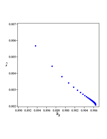
Figure 22: The spectral index and the tensor to scalar ratio for various values.

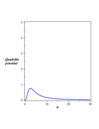
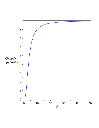
Figure 23: The quadratic and quartic potentials versus the scalar field in Einstein frame. In this frame quadratic potential has a maximum and inflation can occur just for those values of the scalar field located in the left side of the maximum.

From equations (139) and (146) and by using equations (177) and (178) we find the scalar spectral index and the tensor to scalar ratio at $\varphi=\varphi_{hc}$. In figure 22 we have depicted the scalar spectral index and tensor to scalar ratio in a plot for various values of $\xi$ (we started with $\xi=\frac{1}{10}$ corresponding to the first point of the left hand side and then in each step, we increased the value of $\xi$ by $\frac{1}{10}$). This figure shows that as $\xi$ increases, the scalar spectral index becomes larger but the tensor to scalar ratio gets smaller. By increasing $\xi$, $\hat{n}_{s}$ and $\hat{r}$ tend to $0.906$ and $0.002$ respectively (see a similar treatment for the non-minimal Higgs boson as the inflaton in Einstein frame in Park (2008)).

It should be noticed that we don’t consider the case with a quadratic potential here, because this potential in the large scalar field regime tends to zero and there is no inflation for the model in this regime. It is due to the behavior of the quadratic potential in Einstein frame (see figure 23). In Einstein frame, there is a maximum for a quadratic potential that the slow-roll conditions cannot be satisfied beyond it. But for a quartic potential in Einstein frame the situation is different. In the large scalar field regime, the quartic potential tends to a constant and of course the slow-roll conditions can be satisfied.

IX Conclusion

In this paper we have studied the cosmological inflation on the warped DGP braneworld, where a scalar field is non-minimally coupled to the induced gravity term on the brane. We considered the warped DGP setup since this braneworld scenario contains both UV and IR modifications of the general relativity simultaneously. We have studied the inflationary dynamics on the brane both in Jordan and Einstein frame. We have calculated the inflation parameters and perturbations in these two frames with details. In Jordan frame, the brane world nature of the setup and the effects of the non-minimal coupling between the scalar field and induced gravity on the brane is manifest through the existence of some correctional factors in slow-roll parameters. In Einstein frame, the effect of the non-minimal coupling is implicit in the field equations and can be manifested through the conformal transformation between two frames.

Table 5: Am analogy between Einstein an Jordan frame.

Jordan frame                                                           Einstein frame

$\xi=\frac{1}{12}\hskip 42.67912pt\xi=\frac{1}{12}\hskip 39.83368pt\xi=\frac{1}{12}$                         $\xi=\frac{1}{12}\hskip 42.67912pt\xi=\frac{1}{12}\hskip 42.67912pt\xi=\frac{1}{12}$

$n_{s}$       0.9667051476  0.9653928105  0.9665654212                  0.9999999997  1.000000001  0.9999999991

red-tilted         red-tilted        red-tilted                       red-tilted        blue-tilted        red-tilted

$V\propto\varphi^{2}$      $r$        0.1575567389  0.2094435340  0.3137965930                       $\sim 10^{-68}$         $\sim 10^{-68}$         $\sim 10^{-69}$

$\alpha$         $\sim-10^{-51}$       $\sim-10^{-51}$         $\sim-10^{-51}$                       $\sim-10^{-216}$       $\sim-10^{-217}$       $\sim-10^{-217}$

$n_{s}$       1.000000000  0.9999999999  0.9999999996                  0.9999999985  0.9999999995  0.9999999995

scale-invariant       red-tilted        red-tilted                         red-tilted        red-tilted        red-tilted

$V\propto\varphi^{4}$     $r$           $\sim 10^{-21}$          $\sim 10^{-20}$          $\sim 10^{-20}$                        $\sim 10^{-19}$          $\sim 10^{-21}$            $\sim 10^{-22}$

$\alpha$           $\sim-10^{-38}$       $\sim-10^{-38}$         $\sim-10^{-38}$                      $\sim-10^{-162}$       $\sim-10^{-163}$       $\sim-10^{-163}$

The perturbations in these two frames are studied with details. The adiabatic perturbations are generated if the inflaton field is the only field in inflation period. But, if there is more than one scalar field in a model or a scalar field interacts with other fields such as the induced gravity on the brane, the isocurvature perturbations are generated. In our case and in Jordan frame, the presence of the non-minimal coupling between the inflaton field and induced gravity on the brane and also the presence of the non-local effects through the projection of the Weyl tensor on the brane lead to a non-vanishing $\dot{\zeta}$ which affects the primordial spectrum of perturbations. However, in Einstein frame (despite implicit presence of the non-minimal coupling), isocurvature perturbations are generated due to the presence of the non-local effects through the projection of the Weyl tensor on the brane. If we neglect this term in Friedmann equation, the perturbations become adiabatic since neglecting the non-local effect leads to the condition $\frac{\delta\hat{\varphi}}{(d\hat{\varphi})/(d\hat{t})}=\frac{\delta\hat{\rho}_{eff}}{(d\hat{\rho}_{eff})/(d\hat{t})}$ to be satisfied.

By adopting two types of potential ($V=\frac{b}{2m}\varphi^{2m}$; $m=1,2$), we have performed numerical analysis of the model parameters space in each case, the results of which are shown in numerous tables and figures. We note that all of our numerical analysis are done for normal branch of this DGP-inspired model which is essentially ghost-free. In Jordan frame, both for quadratic and quartic potential, all considered parameters ($\epsilon$, $\eta$, $n_{s}$, $n_{T}$, $\alpha$ and $r$) in the large scalar field regime evolve similar to what they do in 4D. In this frame, as $\xi$ becomes larger, the 4D behavior of these parameters lasts in a wider domain of the scalar field values. By more reduction of the scalar field, the evolution of the parameters deviate from the standard 4D behavior. It seems that this deviation from the standard 4D behavior is due to the presence of the tension term in the correctional factors. Of course, with a quartic potential, the parameters experience another standard 4D behavior in the small scalar field regime. But, their values is very different from the values of the corresponding parameters in 4D case.

In Einstein frame, the situation for two types of potentials is much different. With a quartic potential in Einstein frame, the considered parameters in the large scalar field regime have standard 4D behavior (similar to the quartic potential in Jordan frame). In the small scalar field limit, the evolution of the parameters deviate from standard 4D behavior. In this case, as $\xi$ increases, the parameters mimic the standard 4D behavior in a relatively wider domain of the scalar field values. Due to the shape of a quadratic potential in Einstein frame, it is impossible to have inflation in the large scalar field regime. But, when the scalar field is confined to an intermediate regime, the slow-roll conditions can be satisfied and the inflationary phase can be occurred. We note that with a quadratic potential in Jordan frame, the inflationary phase occurs in the large scalar field regime. In this case, the parameter in the intermediate regime have the 4D behavior and in the large and small scalar field regimes they deviate from the standard 4D behavior considerably. Also, as $\xi$ increases, the 4D behavior of all inflation parameters lasts in a wider domain of the scalar field values. In general, with a quartic potential in both Jordan and Einstein frame and with a quadratic potential just in Jordan frame, by increasing of $\xi$ the 4D behavior of parameters lasts in larger domain of the scalar field values. But, with a quadratic potential in Einstein frame, 4D behavior lasts in a wider domain of the scalar field for the smaller values of $\xi$.

We noticed that our analysis shows that although with a quadratic potential in Jordan frame the slow-roll parameters are always positive, with a quartic potential these parameters can be negative for some values of the scalar field. Of course, in Einstein frame both with quadratic and quatic potential, the slow-roll parameters can get negative values.

We have also calculated some inflation parameters at the time that physical scales had crossed the horizon. We note that for this purpose, our analysis have been performed in the high energy limit ($\rho\gg\lambda$). Also, we have considered three values of $\xi$ in each case. The results of our analysis shows that in the warped DGP model with a quadratic potential in Jordan frame, the scalar perturbation is nearly scale invariant and red-tilted ($0.966\leq n_{s}\leq 1$). In this case, the value of the tensor to scalar ratio at the time of the horizon crossing is smaller than $0.24$ (except for $\xi=\frac{1}{6}$ which has $r\simeq 0.31$ ). The running of the scalar spectral index at the time of horizon crossing, is very close to zero but it is negative as usual. So, with a quadratic potential in Jordan frame, there is relatively good agreement between our results and recent observation, specially for $\xi=\frac{1}{8}$ (the result of WMAP+BAO+H₀ Mean data shows that $n_{s}=0.968\pm 0.012$, $r<0.24(95\%CL$ and $-0.022\pm 0.020$). With a quartic potential in Jordan frame, for $\xi=\frac{1}{6}$, the scalar perturbation is quite scale invariant. But, for other $\xi$, it is nearly scale invariant and red-tilted. With this potential, both the running of the spectral index and the tensor to scalar ratio are very close to zero. Then, we have found the value of $\hat{n}_{s}$, $\hat{r}$ and $\hat{\alpha}$ at the horizon crossing time in Einstein frame. With a quartic potential in Einstein frame, the results are similar to the quartic potential in Jordan frame. The scalar perturbation is nearly scale invariant and red-tilted. Also, the running of the scalar perturbation and the tensor to scalar ratio are very close to zero. With a quadratic potential, $\hat{\alpha}$ and $\hat{r}$ are very close to zero too. With this potential in Einstein frame, the scalar perturbation is nearly scale invariant. But, for $\xi=\frac{1}{8}$, it is blue-tilted and for other $\xi$, it is red-tilted (see table 5 which summarizes all of these points). A careful inspection of these results shows that by adopting a quadratic potential and working in Jordan frame, the results of our analysis are more reliable in comparison with recent observations. On the other hand, as table 5 shows, the two frames are not equivalent generally on physical ground. This is an important results. We emphasize that the distinction between the various conformal frames would be unphysical if one were dealing with conformal (Weyl) gravity which is conformally invariant. Since general relativity is not conformally invariant, our discussion entails the use of compensator fields (like the dilaton) whose role is to basically absorb the violations of conformal invariance. Inclusion of such fields in our case helped us to address the comparative analysis of cosmological perturbations in the Jordan and Einstein frames.

In section $8$ we have considered a special case where we have neglected the dark radiation term in the Friedmann equation and therefore the condition for adiabatic perturbation is satisfied. We have considered the inflation parameters of the model in adiabatic condition. Then we have repeated our analysis in the large scalar field regime. Since in this regime, there was no inflationary phase with a quadratic potential in Einstein frame, we have considered only a quartic potential which is nearly constant in the large scalar field regime. With this choice, the braneworld nature of the model affects the standard form of the slow-roll parameters (and so, other inflation parameters) with a constant factor. For the various values of $\xi$, we have found the values of $\hat{n}_{s}$ and $\hat{r}$ at the time of horizon crossing. The results are shown in figure $21$. By increment of $\xi$, the scalar spectral index and tensor to scalar ratio is saturated to $0.906$ and $0.002$ respectively.

Appendix A Jordan Frame, m=1

$$N=-\frac{1}{4}\,{\frac{\kappa_{4}^{2}\left(4\,\kappa_{4}^{2}\sqrt{2}\sqrt{-\varphi_{hc}^{2}\left(-b+8\,{\xi}^{2}R-8\,\xi\,b\right)}-\varphi_{hc}^{2}\kappa_{5}^{2}b+8\,\varphi_{hc}^{2}\kappa_{5}^{2}{\xi}^{2}R-8\,\varphi_{hc}^{2}{\kappa}^{2}\xi\,b\right)}{\kappa_{5}^{2}\left(\xi\,R-b\right)}}$$

Appendix B Jordan Frame, m=2

$$N=\Big{(}1+16\xi\Big{)}\Big{(}\frac{\kappa_{4}^{4}}{\kappa_{5}^{2}\varphi_{hc}}\Big{)}\sqrt{\frac{b\,\varphi_{hc}^{4}-16\,{\xi}^{2}\varphi_{hc}^{2}R+16\,\xi\,\varphi_{hc}^{4}b}{(b\,\varphi_{hc}^{2}-16\,{\xi}^{2}R+16\,\xi\,\varphi_{hc}^{2}b)(b+16\,\xi\,b)}}\hskip 256.0748pt$$

$$\times\ln\Big{(}{\frac{\varphi_{hc}\,b+16\,\xi\,\varphi_{hc}\,b+\sqrt{b\,\varphi_{hc}^{2}-16\,{\xi}^{2}R+16\,\xi\,\varphi_{hc}^{2}b}\sqrt{b+16\,\xi\,b}}{\sqrt{b+16\,\xi\,b}}}\Big{)}\hskip 256.0748pt$$

$$-\frac{\xi R}{2}\Big{(}\frac{\kappa_{4}^{4}}{\kappa_{5}^{2}\varphi_{hc}}\Big{)}\sqrt{\frac{b\,\varphi_{hc}^{4}-16\,{\xi}^{2}\varphi_{hc}^{2}R+16\,\xi\,\varphi_{hc}^{4}b}{(b\,\varphi_{hc}^{2}-16\,{\xi}^{2}R+16\,\xi\,\varphi_{hc}^{2}b)b\,\xi^{2}\,R^{2}}}\hskip 321.51622pt$$

$$\times\Bigg{\{}\ln\Big{(}-2b\,{\frac{\sqrt{b\,\xi\,R}\varphi_{hc}+16\,\sqrt{b\,\xi\,R}\varphi_{hc}\,\xi-16\,{\xi}^{2}R+\sqrt{\xi\,R}\sqrt{b\,\varphi_{hc}^{2}-16\,{\xi}^{2}R+16\,\xi\,\varphi_{hc}^{2}b}}{-\varphi_{hc}b+\sqrt{b\,\xi\,R}}}\,\,\Big{)}\hskip 156.49014pt$$

$$-\ln\Big{(}2b\,{\frac{-\sqrt{b\,\xi\,R}\varphi_{hc}-16\,\sqrt{b\,\xi\,R}\varphi_{hc}\xi-16\,{\xi}^{2}R+\sqrt{\xi\,R}\sqrt{b\,\varphi_{hc}^{2}-16\,{\xi}^{2}R+16\,\xi\,\varphi_{hc}^{2}b}}{\varphi_{hc}b+\sqrt{b\,\xi\,R}}}\,\,\Big{)}\Bigg{\}}\hskip 159.3356pt$$

$$-\frac{1}{8}\,\kappa_{4}^{2}\varphi_{hc}^{2}-2\,\kappa_{4}^{2}\xi\,\varphi_{hc}^{2}-\frac{1}{8}\,{\frac{\kappa_{4}^{2}\xi\,R\ln\left(\xi\,R-b\,\varphi_{hc}^{2}\right)}{b}}\hskip 113.81102pt$$

Appendix C Einstein Frame, m=1

$$N=\Bigg{[}-\frac{1}{4}+54\kappa_{4}^{2}\xi^{4}\varphi_{hc}^{2}-\frac{3}{4}\xi+9\xi^{2}-\frac{9}{2}\kappa_{4}^{2}\xi^{2}\varphi_{hc}^{2}-\frac{1}{2}\kappa_{4}^{2}\xi\varphi_{hc}^{2}-18\kappa_{4}^{4}\xi^{4}\varphi_{hc}^{4}+27\kappa_{4}^{4}\xi^{5}\varphi_{hc}^{4}-\frac{15}{4}\kappa_{4}^{4}\xi^{3}\varphi_{hc}^{4}\hskip 71.13188pt$$

$$-\frac{1}{4}\kappa_{4}^{4}\xi^{2}\varphi_{hc}^{4}\Bigg{]}M-\Bigg{[}\frac{U}{4}-\frac{W}{4}-\frac{3}{2}W-12\kappa_{4}^{2}W-\frac{1}{4}\kappa_{4}^{2}W+12\kappa_{4}^{2}U+\frac{3}{2}U+\frac{1}{4}\kappa_{4}^{2}U\Bigg{]}E+\Bigg{[}396\sqrt{2}\frac{\kappa_{4}^{6}}{\kappa_{5}^{2}}\xi^{4}\varphi_{hc}^{5}\hskip 68.28644pt$$

$$+1188\sqrt{2}\frac{\kappa_{4}^{6}}{\kappa_{5}^{2}}\xi^{5}\varphi_{hc}^{5}+\frac{7\sqrt{2}}{3}\frac{\kappa_{4}^{2}}{\kappa_{5}^{2}}\varphi_{hc}+57\sqrt{2}\frac{\kappa_{4}^{6}}{\kappa_{5}^{2}}\xi^{3}\varphi_{hc}^{5}+3\sqrt{2}\frac{\kappa_{4}^{6}}{\kappa_{5}^{2}}\xi^{2}\varphi_{hc}^{5}+69\sqrt{2}\frac{\kappa_{4}^{4}}{\kappa_{5}^{2}}\xi^{2}\varphi_{hc}^{3}+5\sqrt{2}\frac{\kappa_{4}^{4}}{\kappa_{5}^{2}}\xi\varphi_{hc}^{3}\hskip 88.2037pt$$

$$+306\sqrt{2}\frac{\kappa_{4}^{4}}{\kappa_{5}^{2}}\xi^{3}\varphi_{hc}^{3}+69\sqrt{2}\frac{\kappa_{4}^{4}}{\kappa_{5}^{2}}\xi^{2}\varphi_{hc}^{3}+324\sqrt{2}\frac{\kappa_{4}^{4}}{\kappa_{5}^{2}}\xi^{4}\varphi_{hc}^{3}+36\sqrt{2}\frac{\kappa_{4}^{2}}{\kappa_{5}^{2}}\xi^{2}\varphi_{hc}+108\sqrt{2}\frac{\kappa_{4}^{2}}{\kappa_{5}^{2}}\xi^{3}\varphi_{hc}+\frac{\sqrt{2}}{3}\frac{\kappa_{4}^{8}}{\kappa_{5}^{2}}\xi^{3}\varphi_{hc}^{7}\hskip 65.44142pt$$

$$+54\sqrt{2}\frac{\kappa_{4}^{8}}{\kappa_{5}^{2}}\xi^{5}\varphi_{hc}^{7}+180\sqrt{2}\frac{\kappa_{4}^{8}}{\kappa_{5}^{2}}\xi^{6}\varphi_{hc}^{7}+7\sqrt{2}\frac{\kappa_{4}^{8}}{\kappa_{5}^{2}}\xi^{4}\varphi_{hc}^{7}+216\sqrt{2}\frac{\kappa_{4}^{8}}{\kappa_{5}^{2}}\xi^{7}\varphi_{hc}^{7}+648\sqrt{2}\frac{\kappa_{4}^{4}}{\kappa_{5}^{2}}\xi^{5}\varphi_{hc}^{3}+19\sqrt{2}\frac{\kappa_{4}^{2}}{\kappa_{5}^{2}}\xi\varphi_{hc}\hskip 65.44142pt$$

$$+1296\sqrt{2}\frac{\kappa_{4}^{6}}{\kappa_{5}^{2}}\xi^{6}\varphi_{hc}^{5}\Bigg{]}Q-\Bigg{[}49\sqrt{2}\kappa_{4}^{2}\varphi_{hc}(U+W)+\sqrt{2}\kappa_{4}^{4}\xi\varphi_{hc}^{3}(U+W)+108\sqrt{2}\kappa_{4}^{4}\xi^{3}\varphi_{hc}^{3}(U+W)\hskip 93.89418pt$$

$$+18\sqrt{2}\kappa_{4}^{4}\xi^{2}\varphi_{hc}^{3}(U+W)+216\sqrt{2}\kappa_{4}^{4}\xi^{4}\varphi_{hc}^{3}(U+W)\Bigg{]}Y-\Bigg{[}1188\kappa_{4}^{4}\xi^{5}+1296\kappa_{4}^{4}\xi^{6}+396\kappa_{4}^{4}\xi^{4}+57\kappa_{4}^{4}\xi^{3}\hskip 71.13188pt$$

$$+3\kappa_{4}^{4}\xi^{2}+3564\kappa_{4}^{6}\xi^{6}\varphi_{hc}^{2}+8424\kappa_{4}^{6}\xi^{7}\varphi_{hc}^{2}+7776\kappa_{4}^{6}\xi^{8}\varphi_{hc}^{2}+738\kappa_{4}^{6}\xi^{5}\varphi_{hc}^{2}+75\kappa_{4}^{6}\xi^{4}\varphi_{hc}^{2}+3\kappa_{4}^{6}\xi^{3}\varphi_{hc}^{2}\Bigg{]}DG\hskip 36.98866pt$$

where

$$U=\ln\left(4\,{\frac{\kappa_{4}^{2}\xi\,\left(1-6\,\sqrt{\kappa_{4}^{2}\xi}\varphi_{hc}\,\xi-\sqrt{\kappa_{4}^{2}\xi}\varphi_{hc}+\sqrt{1+3\,\xi}\sqrt{2+2\,\kappa_{4}^{2}\xi\,\varphi_{hc}^{2}+12\,\kappa_{4}^{2}{\xi}^{2}\varphi_{hc}^{2}}\right)}{\kappa_{4}^{2}\xi\,\varphi_{hc}+\sqrt{\kappa_{4}^{2}\xi}}}\right)\hskip 133.72786pt$$

$$W=\ln\left(-4\,{\frac{\kappa_{4}^{2}\xi\,\left(1+6\,\sqrt{\kappa_{4}^{2}\xi}\varphi_{hc}\,\xi+\sqrt{\kappa_{4}^{2}\xi}\varphi_{hc}+\sqrt{1+3\,\xi}\sqrt{2+2\,\kappa_{4}^{2}\xi\,\varphi_{hc}^{2}+12\,\kappa_{4}^{2}{\xi}^{2}\varphi_{hc}^{2}}\right)}{-\kappa_{4}^{2}\xi\,\varphi_{hc}+\sqrt{\kappa_{4}^{2}\xi}}}\right)\hskip 122.34692pt$$

$$D=\ln\left(\sqrt{2\,\kappa_{4}^{2}\xi+12\,\kappa_{4}^{2}{\xi}^{2}}\varphi_{hc}+\sqrt{2+2\,\kappa_{4}^{2}\xi\,\varphi_{hc}^{2}+12\,\kappa_{4}^{2}{\xi}^{2}\varphi_{hc}^{2}}\right)\hskip 244.69386pt$$

$$M=\frac{\kappa_{4}^{3}\varphi_{hc}}{\left(1+3\,\xi\right)\left(6\,\xi+1\right)\left(1+\kappa_{4}^{2}\xi\,\varphi_{hc}^{2}\right)^{3}\left({\frac{1+\kappa_{4}^{2}\xi\,\varphi_{hc}^{2}+6\,\kappa_{4}^{2}{\xi}^{2}\varphi_{hc}^{2}}{\left(1+\kappa_{4}^{2}\xi\,\varphi_{hc}^{2}\right)^{2}}}\right)^{3/2}}\hskip 244.69386pt$$

$$E=\frac{\kappa_{4}^{3}\sqrt{2+2\,\kappa_{4}^{2}\xi\,\varphi_{hc}^{2}+12\,\kappa_{4}^{2}{\xi}^{2}\varphi_{hc}^{2}}}{\left(1+3\,\xi\right)^{3/2}{\sqrt{\kappa_{4}^{2}\xi}}\left(6\,\xi+1\right)\left(1+\kappa_{4}^{2}\xi\,\varphi_{hc}^{2}\right)^{3}\left({\frac{1+\kappa_{4}^{2}\xi\,\varphi_{hc}^{2}+6\,\kappa_{4}^{2}{\xi}^{2}\varphi_{hc}^{2}}{\left(1+\kappa_{4}^{2}\xi\,\varphi_{hc}^{2}\right)^{2}}}\right)^{3/2}}\hskip 210.55022pt$$

$$Q=\frac{\kappa_{4}^{3}\sqrt{2+2\,\kappa_{4}^{2}\xi\,\varphi_{hc}^{2}+12\,\kappa_{4}^{2}{\xi}^{2}\varphi_{hc}^{2}}}{{\sqrt{\kappa_{4}^{2}\xi}}\left(6\,\xi+1\right)^{2}\left(1+\kappa_{4}^{2}\xi\,\varphi_{hc}^{2}\right)^{4}\left({\frac{1+\kappa_{4}^{2}\xi\,\varphi_{hc}^{2}+6\,\kappa_{4}^{2}{\xi}^{2}\varphi_{hc}^{2}}{\left(1+\kappa_{4}^{2}\xi\,\varphi_{hc}^{2}\right)^{2}}}\right)^{3/2}\left(1+3\,\xi\right)\sqrt{{\frac{b\,\varphi_{hc}^{2}}{\left(1+\kappa_{4}^{2}\xi\,\varphi_{hc}^{2}\right)^{2}}}}}\hskip 156.49014pt$$

$$Y=\frac{\kappa_{4}^{3}\sqrt{2+2\,\kappa_{4}^{2}\xi\,\varphi_{hc}^{2}+12\,\kappa_{4}^{2}{\xi}^{2}\varphi_{hc}^{2}}}{\kappa_{5}^{2}\left(1+3\,\xi\right)^{3/2}{\sqrt{\kappa_{4}^{2}\xi}}\left(6\,\xi+1\right)^{2}\left(1+\kappa_{4}^{2}\xi\,\varphi_{hc}^{2}\right)^{4}\left({\frac{1+\kappa_{4}^{2}\xi\,\varphi_{hc}^{2}+6\,\kappa_{4}^{2}{\xi}^{2}\varphi_{hc}^{2}}{\left(1+\kappa_{4}^{2}\xi\,\varphi_{hc}^{2}\right)^{2}}}\right)^{3/2}\sqrt{{\frac{b\,\varphi_{hc}^{2}}{\left(1+\kappa_{4}^{2}\xi\,\varphi_{hc}^{2}\right)^{2}}}}}\hskip 130.88284pt$$

$$G=\frac{\kappa_{4}^{3}\sqrt{2+2\,\kappa_{4}^{2}\xi\,\varphi_{hc}^{2}+12\,\kappa_{4}^{2}{\xi}^{2}\varphi_{hc}^{2}}}{\left(1+3\,\xi\right){\sqrt{\kappa_{4}^{2}\xi}}\left(6\,\xi+1\right)\left(2\,\kappa_{4}^{2}\xi+12\,\kappa_{4}^{2}{\xi}^{2}\right)^{5/2}\left(1+\kappa_{4}^{2}\xi\,\varphi_{hc}^{2}\right)^{3}\left({\frac{1+\kappa_{4}^{2}\xi\,\varphi_{hc}^{2}+6\,\kappa_{4}^{2}{\xi}^{2}\varphi_{hc}^{2}}{\left(1+\kappa_{4}^{2}\xi\,\varphi_{hc}^{2}\right)^{2}}}\right)^{3/2}}\hskip 133.72786pt$$

Appendix D Einstein Frame, m=2

$$N=\frac{1}{64}\frac{\kappa_{4}^{2}}{{\left(6\,\xi+1\right)^{5/2}\kappa_{5}^{2}\sqrt{1+\kappa_{4}^{2}\xi\,\varphi_{hc}^{2}+6\,\kappa_{4}^{2}{\xi}^{2}\varphi_{hc}^{2}}\sqrt{\xi}\sqrt{b}}}\Bigg{[}\Big{(}288\,{\xi}^{2}\sqrt{b}\kappa_{5}{2}+96\,\kappa_{4}^{4}{\xi}^{2}-1152\,\kappa_{4}^{4}{\xi}^{3}+12\,\kappa_{4}^{4}\xi\hskip 65.44142pt$$

$$+\sqrt{b}\kappa_{5}{2}\Big{)}\Pi+\Big{(}576\sqrt{b}\kappa_{5}{2}\xi^{2}+192\,\kappa_{4}^{4}\xi^{2}-2304\,\kappa_{4}^{4}{\xi}^{3}+24\,\kappa_{4}^{4}\xi+2\sqrt{b}\kappa_{5}{2}\Big{)}\Theta+\Big{(}576\,\kappa_{4}^{4}{\xi}^{4}\varphi_{hc}^{4}+192\,\kappa_{4}^{4}{\xi}^{3}\varphi_{hc}^{4}\hskip 54.06006pt$$

$$+16\,\kappa_{4}^{4}{\xi}^{2}\varphi_{hc}^{4}+1152\,\kappa_{4}^{2}{\xi}^{3}\varphi_{hc}^{2}+528\,\kappa_{4}^{2}{\xi}^{2}\varphi_{hc}^{2}+56\,\kappa_{4}^{2}{\xi}\varphi_{hc}^{2}-13824{\xi}^{3}+192\xi+40\Big{)}\Xi+\Big{(}-144\,\kappa_{4}^{4}{\xi}^{4}\varphi_{hc}^{4}\hskip 66.86414pt$$

$$-48\,\kappa_{4}^{4}{\xi}^{3}\varphi_{hc}^{4}-4\,\kappa_{4}^{4}{\xi}^{2}\varphi_{hc}^{4}-36\,\kappa_{4}^{2}{\xi}^{2}\varphi_{hc}^{2}-6\,\kappa_{4}^{2}{\xi}\varphi_{hc}^{2}-2\Delta-576{\xi}^{2}\Big{)}\Delta\Bigg{]}\hskip 170.71652pt$$

where

$$\Theta=\sqrt{1+\kappa_{4}^{2}\xi\,\varphi_{hc}^{2}+6\,\kappa_{4}^{2}{\xi}^{2}\varphi_{hc}^{2}}\ln\left(\kappa_{4}\,\sqrt{\xi}\sqrt{6\,\xi+1}\varphi_{hc}+\sqrt{1+\kappa_{4}^{2}\xi\,\varphi_{hc}^{2}+6\,\kappa_{4}^{2}{\xi}^{2}\varphi_{hc}^{2}}\right)\hskip 103.28363pt$$

$$\Pi=\sqrt{1+\kappa_{4}^{2}\xi\,\varphi_{hc}^{2}+6\,\kappa_{4}^{2}{\xi}^{2}\varphi_{hc}^{2}}\ln\left(2\right)\hskip 312.9803pt$$

$$\Xi=\kappa_{4}^{5}{\xi}^{3/2}\varphi_{hc}\,\sqrt{6\,\xi+1}\hskip 369.88582pt$$

$$\Delta=\varphi_{hc}\,\kappa_{4}\,\sqrt{\xi}\sqrt{6\,\xi+1}\sqrt{b}\kappa_{5}^{2}\hskip 341.43306pt$$

References

- Guth (1981) A. Guth, Phys. Rev. D, 62, 105030, (1981).
- Linde (1982) A. D. Linde, Phys. Lett. B, 108, 389 (1982)
- Albrecht (1982) A. Albrecht and P. Steinhard, Phys. Rev. D, 48, 1220, (1982)
- Linde (1990) A. D. Linde, Particle Physics and Inflationary Cosmology (Harwood Academic Publishers, Chur, Switzerland, 1990).
- Liddle (2000a) A. Liddle and D. Lyth, Cosmological Inflation and Large-Scale Structure, (Cambridge University Press, 2000).
- Lidsey (1997) J. E. Lidsey et al, Phys. Rev. D, 69, 373, (1997).
- Riotto (2002) A. Riotto, [arXiv:hep-ph/0210162].
- Lyth (2009) D. H. Lyth and A. R. Liddle, The Primordial Density Perturbation (Cambridge University Press, 2009).
- Brandenberger (2005) R. H. Brandenberger, [arXiv:hep-th/0509099].
- Lidsey (2004) J. E. Lidsey, Lect. Notes Phys., 646, 357, (2004).
- Buchel (2004) A. Buchel and A. Ghodsi, Phys. Rev. D, 70, 126008, (2004).
- Dvali (2000) G. Dvali, G. Gabadadze and M. Porrati, Phys. Lett. B, 485, 208, (2000).
- Dvali (2001a) G. Dvali and G. Gabadadze, Phys. Rev. D, 63, 065007, (2001a).
- Dvali (2001b) G. Dvali, G. Gabadadze, M. Kolanovic and F. Nitti, Phys. Rev. D, 64, 084004, (2001b).
- Lue (2006) A. Lue, Phys. Rept., 423, 1, (2006).
- Lazkoz (2004) R. Lazkoz, Phys. Rev. D, 70, 064033, (2004).
- Corradini (2008) O. Corradini and A. Iglesias, JCAP, 0805, 012, (2008).
- Randall (1999) L. Randall and R. Sundrum, Phys. Rev. Lett., 83, 4690, (1999).
- Maeda (2003) Kei-ichi Maeda, S. Mizuno and T. Torii, Phys. Rev. D, 68, 024033, (2003).
- Cai (2004) R. -G. Cai and H. Zhang, JCAP, 08, 017, (2004).
- Zhang (2006) H. Zhang and Z. -H. Zhu, Phys. Lett. B, 641, 405, (2006).
- Nozari (2007a) K. Nozari and B. Fazlpour, JCAP, 11, 006, (2007a).
- Nozari (2011) K. Nozari, M. Shoukrani and B. Fazlpour, Gen. Rel. Grav, 43, 207, (2011).
- Langlois (2000) D. Langlois, R. Maartens and D. Wands, Phys. Lett. B, 489, 259, (2000).
- Langlois (2007) D. Langlois and F. Vernizzi, JCAP, 02, 017, (2007).
- Bouhamdi-Lopez (2004) M. Bouhmadi-Lopez, R. Maartens and D. Wands, Phys. Rev. D, 70, 123519, (2004).
- Kaloper (2005) N. Kaloper, Phys. Rev. D, 71, 086003, (2005).
- Nozari (2007b) K. Nozari, JCAP, 0709, 003, (2007b).
- Faraoni (1996) V. Faraoni, Phys. Rev. D, 53, 6813, (1996).
- Faraoni (2000) V. Faraoni, Phys. Rev. D, 62, 023504, (2000).
- Faraoni (1999) V. Faraoni, Int. J. Theor. Phys., 38, 217, (1999).
- Spokoiny (1984) B. L. Spokoiny, Phys. Lett. B, 147, 39, (1984).
- Futamase (1989) T. Futamase and K. I. Maeda, Phys. Rev. D, 39, 399, (1989).
- Salopek (1989) D. S. Salopek, J. R. Bond and J. M. Bardeen, Phys. Rev. D, 40, 1753, (1989).
- Fakir (1990) R. Fakir and W. G. Unruh, Phys. Rev. D, 41, 1783, (1990).
- Schimd (2005) C. Schimd, J. P. Uzan and A. Riazuelo, Phys. Rev. D, 71, 083512, (2005).
- Makino (1991) N. Makino and M. Sasaki, Prog. Theor. Phys., 86, 103, (1991).
- Fakir (1992) R. Fakir, S. Habib and W. G. Unruh, Astrophys. J., 394, 396, (1992).
- Libanov (1998) M. V. Libanov, V. A. Rubakov and P. G. Tinyakov, Phys. Lett. B, 442, 63, (1998).
- Hwang (1999) J. Hwang and H. Noh, Phys. Rev. D, 60, 123001, (1999).
- Hwang (1998) J. Hwang and H. Noh, Phys. Rev. Lett., 81, 5274, (1998).
- Tsujikawa (1999a) S. Tsujikawa, K. Maeda and T. Torii, Phys. Rev. D, 60, 063515, (1999a).
- Tsujikawa (1999b) S. Tsujikawa, K. Maeda and T. Torii, Phys. Rev. D, 60, 123505, (1999b).
- Tsujikawa (2000a) S. Tsujikawa, Phys. Rev. D, 62, 043512, (2000a).
- Chiba (2000) T. Chiba and M. Yamaguchi, Phys. Rev. D, 61, 027304, (2000).
- Tsujikawa (2000b) S. Tsujikawa and H. Yajima, Phys. Rev. D, 62, 123512, (2000b).
- Gunzig (2001) E. Gunzig, A. Saa, L. Brenig, V. Faraoni, T. M. Rocha Filho and A. Figueiredo, Phys. Rev. D, 63, 067301, (2001).
- Koh (2005) S. Koh, S. P. Kim and D. J. Song, Phys. Rev. D, 72, 043523, (2005).
- Marco (2006) F. Di Marco and A. Notari, Phys. Rev. D, 73, 063514, (2006).
- Bojowald (2006) M. Bojowald and M. Kagan, Phys. Rev. D, 74, 044033, (2006).
- Bauer (2008) F. Bauer and D. A. Demir, Phys. Lett. B, 665, 222, (2008).
- Easson (2009) D. A. Easson and R. Gregory, Phys. Rev. D, 80, 083518, (2009).
- Hertzberg (2010) M. P. Hertzberg, JHEP, 1011, 023, (2010).
- Pallis (2010) C. Pallis, Phys. Lett. B, 692, 287, (2010).
- Pallis (2011) C. Pallis and N. Toumbas, JCAP, 1102, 019, (2011).
- Kaiser (1995) D. I. Kaiser, Phys. Rev. D, 52, 4295, (1995).
- Chiba (2008) T. Chiba and M. Yamaguchi, JCAP, 0810, 021, (2008).
- Capozziello (1997) S. Capozziello, R. de Ritis and A. Angela Marino, Class. Quant. Grav., 14, 3243, (1997).
- Nandi (1998) K. K. Nandi, B. Bhattacharjee, S. M. K. Alam and J. Evans, Phys. Rev. D, 57, 823, (1998).
- Flanagan (2004) E. E. Flanagan, Class. Quant. Grav., 21, 3817, (2004).
- Bhadra (2007) A. Bhadra, K. Sarkar, D. P. Datta and K. K. Nandi, Mod. Phys. Lett. A, 22, 367, (2007).
- Faraoni (2007) V. Faraoni and S. Nadeau, Phys. Rev. D, 75, 023501, (2007).
- Nozari (2009) K. Nozari and S. D. Sadatian, Mod. Phys. Lett. A, 24, 3143, (2009).
- Capozziello (2010a) S. Capozziello, P. Martin-Moruno and C. Rubano, Phys. Lett. B, 689, 117, (2010a).
- Capozziello (2010b) S. Capozziello, F. Darabi and D. Vernieri, Mod. Phys. Lett. A, 25, 3279, (2010b).
- Quiros (2011a) I. Quiros, R. Garcia-Salcedo, J. Edgar Madriz Aguilar, [arXiv:1108.2911].
- Quiros (2011b) I. Quiros, R. Garcia-Salcedo, J. Edgar Madriz Aguilar and T. Matos, [arXiv:1108.5857].
- Himemoto (2001) Y. Himemoto and M. Sasaki, Phys. Rev. D63, 044015 (2001).
- Himemoto (2003) Y. Himemoto and M. Sasaki, Prog. Theor. Phys. Suppl. 148, 235 (2003).
- Yokoyama (2001) J. Yokoyama and Y. Himemoto, Phys. Rev. D64, 083511 (2001).
- Sasaki (2004) M. Sasaki, PRAMANA J. Phys. 63, 785 (2004).
- Nozari (2012) K. Nozari, M. Khamesian and N. Rashidi, Astropart. Phys. 35, 828 (2012).
- Maartens (2010) R. Maartens and K. Koyama, Living Rev. Relativity, 13, 5, (2010).
- Bardeen (1980) J. Bardeen, Phys. Rev. D, 22, 1882, (1980).
- Mukhanov (1992) V. F. Mukhanov, H. A. Feldman and R. H. Brandenberger, Phys. Rept., 215, 203, (1992).
- Bertschinger (1995) E. Bertschinger, [arXiv:astro-ph/9503125].
- Koyama (2006) K. Koyama and R. Maartens, JCAP, 0601, 016, (2006).
- Langlois (2001) D. Langlois, R. Maartens, M. Sasaki, Phys. Rev. D, 63, 084009, (2001).
- Bassett (1999) B. A. Bassett, F. Tamburini, D. I. Kaiser and R. Maartens, Nucl. Phys. B, 561, 188, (1999).
- Gordon (2001) C. Gordon, D. Wands, B. A. Basset and R. Maartens, Phys. Rev. D, 63, 023506, (2001).
- Maartens (2000) R. Maartens, D. Wands, B. A. Bassett and I. Heard, Phys. Rev. D, 62, 041301, (2000).
- Seahra (2010) S. S. Seahra and W. Hu, Phys. Rev. D, 82, 124015, (2010).
- Bardeen (1983) J. M. Bardeen, P. J. Steinhardt and M. S. Turner, Phys. Rev. D, 28, 679, (1983).
- Wands (2000) D. Wands, K. A. Malik, D. H. Lyth and A. R. Liddle, Phys. Rev. D, 62, 043527, (2000).
- Liddle (2000b) A. R. Liddle and A. Mazumdar, Phys. Rev. D, 61, 123507, (2000b).
- Cid (2007) M. A. Cid, S. Del Campo and R. Herrera, JCAP, 10, 005, (2007).
- Amendola (2006) L. Amendola, C. Charmousis and S. C. Davis, JCAP 0612, 020, (2006).
- Amendola (2007) L. Amendola, C. Charmousis and S. C. Davis, JCAP 0710, 004, (2007).
- Shtanov (2007) Y. Shtanov, A. Viznyuk and V. Sahni, Class. Quant. Grav. 24, 6159, (2007).
- Hiramatsu (2006) T. Hiramatsu and K. Koyama, JCAP 0612, 009, (2006).
- Koyama (2007) K. Koyama et al., JCAP 0704, 001, (2007).
- Koyama (2008) K. Koyama, A. Mennim and D. Wands, Phys. Rev. D, 77, 021501, (2008).
- Stewart (1993) E. D. Stewart and D. H. Lyth, Phys. Lett. B, 302, 171, (1993).
- Koyama (2005) K. Koyama, Phys. Rev. D, 72, 123511, (2005).
- Izumi (2007) K. Izumi, K. Koyama and T. Tanaka, JHEP, 0704, 053, (2007).
- Koyama (2007) K. Koyama, Class. Quantum Grav., 24, R 231, (2007).
- de Rham (2006) C. de Rham and A. J. Tolley, JCAP, 0607, 004, (2006).
- Fujii (2003) Y. Fujii and K. -i. Maeda, The Scalar Tensor Theory of Gravitation (Cambridge University Press, 2003).
- Komatsu (2011) E. Komatsu et al., Astrophys. J. Suppl., 192, 18, (2011).
- Cai (2007) Y. -F. Cai, T. Qiu, Y. -S. Piao, M. Li and X. Zhang, JHEP 0710, 071, (2007).
- Park (2008) S. C. Park and S. Yamaguchi, JCAP, 0808, 009, (2008).